www.ocean-sci.net/7/805/2011/ doi:10.5194/os-7-805-2011
© Author(s) 2011. CC Attribution 3.0 License.
Ocean Science
Usefulness of high resolution coastal models for operational oil spill
forecast: the “Full City” accident
G. Brostr¨om1, A. Carrasco1, L. R. Hole1, S. Dick2, F. Janssen2, J. Mattsson3, and S. Berger4
1Norwegian Meteorological Institute (met.no), Norway 2Federal Maritime and Hydrographic Agency (BSH), Germany 3Danish Maritime Safety Administration (DAMSA), Denmark 4The Norwegian Coastal Administration (NCA), Norway
Received: 1 March 2011 – Published in Ocean Sci. Discuss.: 22 June 2011
Revised: 30 September 2011 – Accepted: 9 October 2011 – Published: 29 November 2011
Abstract.Oil spill modeling is considered to be an important part of a decision support system (DeSS) for oil spill combat-ment and is useful for remedial action in case of accidents, as well as for designing the environmental monitoring system that is frequently set up after major accidents. Many acci-dents take place in coastal areas, implying that low resolution basin scale ocean models are of limited use for predicting the trajectories of an oil spill. In this study, we target the oil spill in connection with the “Full City” accident on the Norwe-gian south coast and compare operational simulations from three different oil spill models for the area. The result of the analysis is that all models do a satisfactory job. The “stan-dard” operational model for the area is shown to have severe flaws, but by applying ocean forcing data of higher resolu-tion (1.5 km resoluresolu-tion), the model system shows results that compare well with observations. The study also shows that an ensemble of results from the three different models is use-ful when predicting/analyzing oil spill in coastal areas.
1 Introduction
Oil spill models are important tools for predictions of oil spill movement and for evaluating their impact on the en-vironment. An accurate prediction is of tremendous value for the organization that is responsible for the cleaning ac-tions and for setting up environmental monitoring programs. Any comprehensive modeling systems for oil spill are intrin-sically complex: besides the full three-dimensional velocity, temperature and salinity fields needed for an adequate de-scription of the advection of the oil spill, the oil chemistry and its interaction with water, waves, bottom, etc., must be
Correspondence to:G. Brostr¨om ([email protected])
described (Castanedo et al., 2006; Dick and M¨uller-Navarra, 2002; Diez et al., 2007; Reed et al., 1999; French-McCay, 2004; Wanga et al., 2008). The complexity of the entire sys-tem implies that many simplifications must be introduced and it is not always clear how these simplifications (e.g. consider-ing two dimensional models only, neglectconsider-ing wave-induced mixing and drift, etc.) will influence the performance of the model.
There have been a number of studies highlighting the ben-efits of comprehensive oil drift modeling systems. For in-stance, models have been used for assessment in a number of different accidents and crisis’s, e.g., the spill in the Arabian Gulf (Proctor et al., 1994; Venkatesh and Murty, 1994), the Prestige accident (Castanedo et al., 2006; Diez et al., 2007; Daniel et al., 2005), the oil spill in the Lebanon crisis (Cop-pini et al., 2011). In addition to direct impact studies of oil spill accidents, there have been a number of important stud-ies on e.g., shipping pathways for risk assessments (Soomere et al., 2010, 2011; Viikm¨ae et al., 2010) showing the impor-tance of oil spill modeling for the community. Most likely, the performance will depend on the exact physical situation during the spill event. In any case, it is safe to state that vali-dation of oil spill models is an important ingredient for eval-uating the performance of the models and that further studies are required for development and testing of model systems.
1.1 “Full City” accident
On 30 July 2009 at around 12:00 UTC (we will use UTC throughout this study) the Panama-registered cargo vessel MV “Full City” anchored on the Norwegian coast about 2 km from the S˚astein Island outside Langesund (Fig. 1) in the Skagerrak area. According to the Accident Investigation Board Norway (AIBN), the “Full City” started to drift to-ward S˚astein Island at about 21:50 due to very strong winds and waves from southwest (AIBN, preliminary report). Both flukes on the anchor broke off and, even though the engines were turned on, the ship remained un-maneuverable. On 30 July at about 22:30 “Full City” ran onto the rocky ground off S˚astein Island (9.716◦E, 58.9671◦N) (Fig. 1). The ship suffered severe hull damage and started to leak heavy bunker oil that polluted the sea and extensive sections of the shore. The ship carried about 1000 tons of heavy bunker oil (IF180 with a density of 994 kg m−3) and 120 tons of marine diesel. It is estimated that about 300 tons of heavy bunker oil were released; preliminary estimates suggest that 200 tons were spilled during the first hours, and the remaining 100 tons over the next 6–8 h. The accident was reported during the night and the oil spill response action was started next morning. It was quickly recognized that it was a significant oil spill in an ecological sensitive area. The accident took place in the main holiday season in a popular area for vacation, and the spill received major attention in news media.
According to the Norwegian Coastal Administration (NCA), oil was observed on 2 August in several areas along the coast (see the discussion in Sect. 3). About 70 km of the coastline were directly polluted by the oil spill, and oil pol-lution was observed at about 190 different locations. Some of the affected fjords are protected areas and bird sanctuar-ies and an extensive monitoring of the environmental con-sequences is still going on. During the days following the incident, hundreds of birds covered in oil were considered beyond saving; totally it is estimated that about 1500–2000 eiders and about 500 additional seabirds were destroyed dur-ing to the accident (Lorentsen et al., 2010).
By 12 August NCA claimed that 860 m3 of oil had been recovered from the ship, 28 m3pure oil from the sea, 74 m3 from the beaches, and 180 tons of oil emulsions had been recovered from the beaches and sea; accordingly, it is esti-mated that about 190 tons of oil remained in the environment (Lorentsen et al., 2010). In all about 15 000–18 000 man-days were spent in the clean-up. The total cost estimated for the remedial action was about 25 m euros, and up to 2 m euros will be used for environmental monitoring until 2014 (Olsen, 2009).
1.2 Weather conditions during the period 1.2.1 Atmospheric conditions
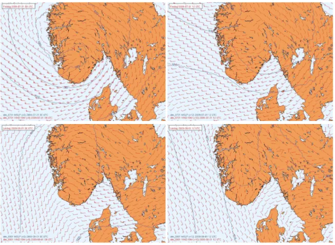
The weather conditions during and immediately after the ac-cident, according to the met.no setup of the High Resolu-tion Local Area Modeling (HIRLAM) model (Und´en et al., 2002), are shown in Fig. 2. An intense low pressure system was located over southern Norway at the time of the acci-dent, which gave rise to strong gale winds in the Skagerrak area parallel to the Norwegian coast. The strong winds pre-vailed a few hours after the “Full City” went aground, but decreased rapidly thereafter. Wind speed data from an ob-servation station at Jomfruland (about 30 km southwest from S˚astein, Fig. 1) show that the wind speed was around 18 m/s and with a direction around 210◦at the time of the accident. The wind remained constant for about 5 h, and then (about 6 h after the accident) it decreased to about 7 m s−1and di-rection turned to 235◦. At 31 July 12:00 the wind turned further to 275◦and decreases slowly with time. From about 11:00 at 1 August, the wind properties (speed about 9 m s−1, direction 220◦) were constant until 2 August when there was a major shift in wind direction to about 60◦ from 06:00 in the morning until about 24:00. It should be noted that in a reanalysis of the fate of the oil spill that was carried out by SINTEF1, the wind speed observations at Jomfruland were used rather than wind speed from the meteorological models as it produced results in better agreement with observations (M. Reed, personal communication, 2010).
1.2.2 Wave conditions
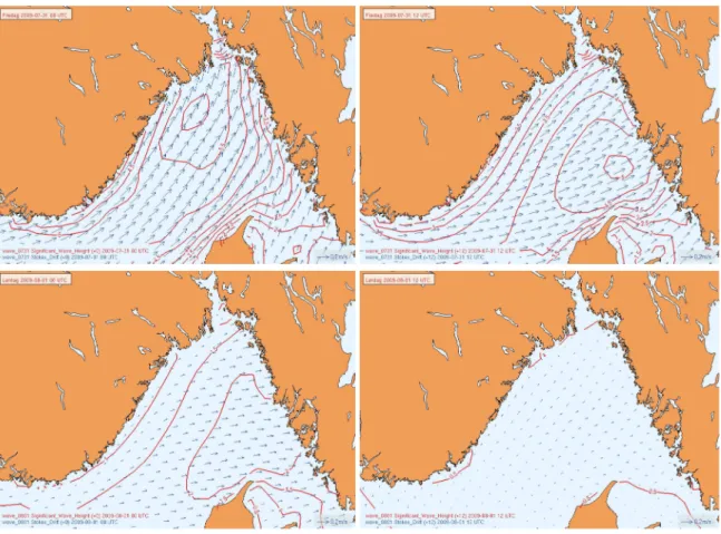
The strong wind blowing along the coast at midnight between 30–31 July gave rise to significant wave heights of order 5– 6 m in the central Skagerrak area, according to the met.no wave model analysis, while the significant wave height along the Norwegian coast reached about 4 m (Fig. 3). Waves con-tribute to particle movement due to the Stokes drift (Phillips, 1977), and there was a significant Stokes drift of order 0.2– 0.3 m s−1towards northeast associated with the strong wave field. The significant wave height declined rapidly when the wind speed decreased, and on 1 August at 06:00 the signifi-cant wave height was about 1 m in the central Skagerrak area. Wave models are in general accurate for open water condi-tions and we expect these simulacondi-tions to be correspondingly good (Komen et al., 1994; Cavaleri et al., 2007). However, the exact wave height at the coast depends on the match of the wind direction and the orientation of the coastline. Local geographic effects, such as wave sheltering and wave refrac-tion, also play a role for the exact wave conditions at the accident site, and these fine-scale structures are not captured by met.no wave model.
1SINTEF is a semi-private non-profitable Norwegian research
Fig. 1. (a)Location of the Island S˚astein in Skagerrak area where the ship “Full City” grounded.(b)Picture of the MV “Full City” outside S˚astein on 2 August. (Photo: NCA).
1.2.3 Current conditions
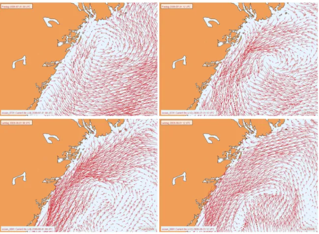
The ocean currents for the period, according to the met.no ocean model with 1.5 km resolution that focuses on Skager-rak and northern North Sea, are outlined in Fig. 4. It should be noted that wind and wave conditions are most likely fairly similar in all models used in this study, the main difference is probably in the ocean models and the various setups of the oil drift models. However, we show the situation from the met.no model for the Skagerrak to exemplify typical cur-rent patterns for the area. For this period, the model simula-tion shows a strong cyclonic current system in the Skagerrak
Fig. 2. The sea level pressure and the wind at the surface from met.no. The fields are from the operational HIRLAM model running with 8 km resolution. Upper left panel is from 31 July at 00:00; upper right panel is from 31 July at 12:00; lower left panel is from 1 August at 00:00; and lower right panel is from 1 August at 12:00.
wind-driven Ekman currents out from the coast and a weak-ened north-eastward coastal jet. Accordingly, the coastal cur-rent most likely returned to more typical conditions with a south-westward buoyancy driven current (i.e. the southward coastal current driven by the steady freshwater output from Baltic Sea and the European rivers, which is a stable current system along the coast of the northern Skagerrak). It is seen that this situation occurs in the met.no ocean model, and it is thus expected that the oil moved towards northeast initially and outwards from the coast after a few hours; after this we expect that the oil moved towards southwest with the reap-pearing coastal current.
1.2.4 Oil drift models
The oil drift models in this study are based on super-particles that are advected by ocean currents and wind impact. The currents can be taken from ocean models or parameteriza-tions of drift speeds. The super-particles also contain de-scriptions of oil chemistry, horizontal dispersion and mixing within the water column. The oil drift models, along with the atmospheric, wave and ocean models that are used the
force them, are described in Sect. 2. In Sect. 3 we describe observations of the oil spill and discuss how the different oil spill models in this study agree with the observations. Given that we only have qualitative observations of the oil spill, we limit the analysis to a simple “show and tell” description. Section 4 is devoted to a discussion of the results.
2 Model descriptions
2.1 Norwegian Metrological Institute model system 2.1.1 Atmosphere and wave models
Fig. 3.Significant wave height (red contours) and Stokes drift velocity vector (blue arrows), from the model WAM4 km. Upper left panel is from 31 July at 00:00; upper right panel is from 31 July at 12:00; lower left panel is from 1 August at 00:00; lower right panel is from 1 August at 12:00.
velocity are calculated at “half” levels. For the horizontal discretisation, an Arakawa C-grid is used. The equations are written for a general map projection, but in practice nor-mally a rotated lat-lon grid projection is adopted. Turbu-lence is described using a prognostic Turbulent Kinetic En-ergy (TKE) scheme (Tijm and Lenderink, 2003). The assim-ilation of observations is mainly done by variational methods combining 3D-VAR (Unden et al., 2002) and 4D-VAR. Bias corrections are applied to most satellite data. Observation screening involves logical and representativity checks, back-ground quality checks, black-or-white listing, multi-level and station level checks, redundancy checks and moving platform checks.
The wave model is based on the wave model project code (WAM) that describes the energy in different wave compo-nents (Komen et al., 1994; Phillips, 1977; Cavalieri, 2007): WAM belongs to the third generation wave models and ac-counts for the non-linear interaction between the wave com-ponents. The Stokes drift is calculated from an integra-tion over the wave spectrum, the contribuintegra-tion from high-frequency waves that are not resolved by the model is
cal-culated using a self-similar spectral shape of this part of the spectrum (Komen et al., 1994; Phillips, 1977). The main un-certainty in the estimate of the Stokes drift is the sensitivity to the relatively unknown high-frequency part of the spectrum (Ardhuin et al., 2009), which may induce uncertainties of up to 50 % under certain conditions. However, compared to the large uncertainties in upper ocean currents, it may be con-sidered as a reliable and well-predicted quantity, especially for direction and in strong wind conditions (Brostr¨om et al., 2009).
2.1.2 Ocean models
Fig. 4. Velocity vectors of surface currents in the ocean from the met.no 1.5 km ocean model. Upper left panel is from 31 July at 00:00; upper right panel is from 31 July at 12:00; lower left panel is from 1 August at 00:00; lower right panel is from 1 August at 12:00.
heat flux formulations have been adjusted for local condi-tions (Røed and Debernard, 2004); the model also includes a simple nudging scheme to assimilate satellite SST products. Tides are included by the eight harmonic components (M2, S2, N2, K2, Q1, O1, P1 and K1) taken from a barotropic tidal model. The tidal forcing is applied at the lateral edge of the model. In this study we use two different setups of the model (i.e. the Skagerrak 1.5 km model that covers Skager-rak and parts of the North Sea and the Nordic 4 km model that covers Nordic Seas and North Sea), they are both on a polar stereographic grid and the results must be interpo-lated onto a regular geographic grid before being used in the oil drift model. For this study, we interpolate forcing onto a grid that has similar resolution as the underlying ocean model; interpolation/extrapolation to a finer grid may affect the beaching pattern of the oil drift model.
2.1.3 Oil drift modeling
The oil drift model at met.no is based on the Oil Drift 3 Di-mensional numerical model (OD3D) that was developed in cooperation with SINTEF (Martinsen et al., 1994; Wettre et al., 2001). OD3D is based on super-particles that represent
the main characteristics of the oil. The particle drift is forced by wind, waves (including the Stokes drift), oceanic currents and stratification. The oil chemistry depends mainly on tem-perature, wind speed and significant wave height. The model time step is 15 min and thus the numerical advection of parti-cles, especially in areas with complex topography, is not very accurate. Furthermore, in the present operational setting, the model does not allow for oil particles to be inside the one-half grid-point closest to the coast, for numerical reasons2. The OD3D model (and the other models in this study) pre-dicts the drift of oil particles, how they disperse in time and how much oil has been evaporated, submerged and beached. In this study, we will focus on the advection, dispersion, and beaching.
2This numerical setting is based on a central differencing
In the “standard” operational setup, OD3D uses forcing data from the Nordic 4 km ocean model. However, it is ex-pected that an ocean model with 4 km resolution will not perform well in the vicinity of rugged sections of the coast-line or/and in archipelago areas. The oil drift model can be driven using various atmospheric, wave, and ocean models in a non-operational mode and in this study we will com-pare the performance using the Nordic 4 km model and the Skagerrak 1.5 km model for the “Full City” accident. Note that OD3D only accepts fields in geographic grids, i.e., in standard longitude-latitude grids. Thus, in order to generate inputs to OD3D all forcing fields must be interpolated to the same latitude-longitude domain.
2.2 BSH model system
The oil spill model of the German Federal Maritime and Hy-drographic Agency (BSH) is part of a decision-support sys-tem (DeSS) for combating marine environmental pollution. The system consists of a hydrodynamical circulation model for the North Sea and Baltic Sea (BSHcmod) and various drift and dispersion models for different substances or ap-plications. The circulation model is three-dimensional and takes into account meteorological conditions in the North Sea and Baltic Sea area, tides and external surges entering the North Sea from the Atlantic, heat fluxes between atmo-sphere and ocean as well as river runoff from the major rivers (Dick et al., 2010). The meteorological forecasts are pro-vided by the COSMO-EU model run at German Weather Ser-vice (DWD). The BSH circulation model predicts tidal, wind and density driven motion up to 84 h ahead on two nested grids. Grid resolution is 900 m in the German Bight and western Baltic Sea, while it is approximately 5 km in other parts of the North Sea and Baltic as well as in the Skagerrak area.
A Lagrangian drift and dispersion model (BSHdmod.L) is used primarily to assist the German Central Command for Maritime Emergencies in cases of marine environmental pol-lution and to support search and rescue operations. Addi-tionally, the model is frequently used to back-track harmful substances and thus has become a valuable tool in the identi-fication of environmental polluters.
In the model, the particular substance is represented by a particle cloud drifting with the current. Sub-scale turbulent motion is simulated by a Monte Carlo method. Substances floating on the surface are additionally driven in direction of the wind with a factor of 2.3 percent of wind velocity. In simulations of oil dispersion, the physical behavior of differ-ent oil types on the water surface and in the water column is also taken into account. The BSH’s oil drift model sim-ulates wind and current induced drift, spreading, horizontal and vertical dispersion, evaporation, emulsification, sinking, beaching as well as the deposition of oil on the sea bed (Dick and Soetje, 1990). Wave effects on drifting and dispersed oil are parameterized by wind velocity. In the BSH model,
a particular oil type consists of seven groups of hydrocarbon compounds and a residuum. In the past years, the models had been used successfully in several cases of oil pollution (Dick and M¨uller-Navarra, 2002).
2.3 DAMSA/SMHI model
The DAMSA/SMHI oil drift model is called Seatrack Web, and is regarded as the HELCOM oil and chemical modeling and drift forecasting system. Seatrack Web covers the Baltic Sea area and the eastern part of the North Sea. The system is available over internet, which enables users to start an oil drift simulation on the server and have the results presented on their local computer.
Seatrack Web consists of three parts. The first part is the operational weather and ocean forecasting system, which provides the necessary wind and current fields. The second part is the drift, spreading and weathering model. The ex-ecution of the model is controlled by the third part of the system, which is the client/server web application. It handles the communication and comprises a graphical user interface (GUI) on the client side and a Java Servlet on the server side.
2.3.1 Wind and ocean fields
Wind and ocean forecasts are taken from the Swedish Me-teorological and Hydrological (SMHI) forecasting systems; i.e. the SMHI setup of HIRLAM atmospheric model and the High Resolution Operational Model for the Baltic Sea (HI-ROMB) ocean model, respectively. HIROMB is run four times a day using forcing fields from HIRLAM with 22 km resolution and produces 48-h forecasts of currents, temper-ature, salinity, and ice conditions for the North Sea–Baltic Sea area. HIROMB calculates current velocities on a reg-ular spherical lat-lon grid with a horizontal resolution of 3 nautical miles (about 5.5 km). In the vertical direction, HI-ROMB usesz-level coordinates with up to 24 layers, rang-ing from a 4 m thick surface layer to a 60 m thick bottom layer at the deepest parts. The Stokes drift is accounted for in Seatrack Web, and calculated based on the wave spec-trum. Currently, the wave spectrum is not imported from an operational wave forecast model. Instead, a parameterised wind-dependent spectrum for fetch-limited growth is used. The HIRLAM and HIROMB forecasts are subsequently pro-cessed and made available for Seatrack Web, in which simu-lations 2 days ahead and 30 days back in time are possible.
2.3.2 Oil drift, spreading and weathering
As the other two models in this study, Seatrack Web uses a particle-tracking technique to model the drift and spreading of oil spills. The spill is divided into an ensemble of discrete particles, initially of equal mass. The particles are advected and dispersed in the three-dimensional velocity and turbu-lence fields, which are discretised in space and time. Algo-rithms for gravitational surface spreading of buoyant oil and vertical dispersion result in additional particle displacements. The properties of oil spilled at sea will change owing to weathering processes. Seatrack Web calculates changes in oil density and viscosity. These parameters are important state variables in relation to cleanup operations, but are also mutually connected to the rate of weathering and spreading. Density and viscosity are diagnostic variables and vary as functions of temperature, evaporated fraction and water frac-tion (in the case of emulsifying oils).
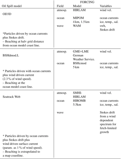
The different models use different forcing and parameter-izations, and the various models are summarized in Table 1.
3 The oil drift experiments
The “Full City” grounded on 30 July at 22:30 (UTC), with a subsequent discharge of around 300 m3of IF 180 oil (which is a heavy bunker oil) over 8 h. The discharge was proba-bly uneven in time with greater discharge in the early part of the accident with about 100 m3discharge in the first hour. However, in this study we simply assume that 300 m3 was released between 30 July 23:00 and 31 July 07:00 at a con-stant rate. The exact point of release was very close to the coast, but the release point will in the models to some extent depend on the model formulation.
The characteristics of the oil release from the ship are fairly well established. However, this was a major release of oil close to the coastline in an area with complex topogra-phy. It is likely that a certain amount of the released oil was initially trapped in the vicinity of the accident site, and its subsequent release to the more open ocean in a later stage is not described in the model systems. Accordingly, it is possi-ble that the modeled oil spill will have a somewhat different release timeline then the actual release of oil from the ship.
3.1 Observations of the spill 3.1.1 Direct observations
We here give a brief description of the oil spill based on ob-servations recorded by the Norwegian Coastal Administra-tion (NCA) and oil samples taken during the response acAdministra-tion. The times of the records refer to the first reported observa-tions. Therefore there might be a time lag from when the oil actually appeared in an area until it was discovered and reported.
Shortly after the grounding, oil slicks drifting northwards were observed. Within few hours oil hit the shore in the area Krogshavn (see Fig. 1 and www.norgeskart.no). On 31 July around 11:00 oil was observed in the area Mølen, soon after also Oddane, a little further east, was affected by the spill. In the evening (around 19:00–20:00), the first indications that oil was drifting southwards from the grounding site were re-ported.
In the early morning on 1 August observations from the public indicate that smaller amounts of oil were drifting south of the island Jomfruland. In the evening drifting oil was observed in the area outside Risør (23 km southwest of Jomfruland just outside the map in Fig. 5). Larger amounts were recorded in the Risør area in the morning of the 2 Au-gust. In the late afternoon oil has stranded at Ruaker, near Grimstad (about 75 km southwest of Jomfruland).
Figure 5 shows all areas where beached oil has been recorded by shoreline surveys and verification of reports from the public, a task that went on for weeks and months. All observations of beached oil regardless of amount are in-cluded in the figure.
3.1.2 Observations by remote sensing
The satellite SAR detection for the oil spill was investigated immediately after the spill by the Nansen Environmental and Remote Sensing Center (NERSC) in Bergen, Norway. How-ever, the impact of the remote sensing capabilities based on SAR images at the time of the accident was reduced due to strong winds and the close proximity of the spill to land or islands. Later, on 4 August, a relatively large area of low backscatter associated with weak winds dominates the im-age in the central Skim-agerrak waters. Closer to the coast dark elongated features become visible. In close proxim-ity of the coast, on the other hand, the spatial backscatter variability is high and without any clear and distinct expres-sions of possible spills. Data from visible-light cameras and IR/UV-sensors, obtained during over-flights, made it possible to establish the nature of numerous dark features. NERSC has demonstrated this in Fig. 6 in which the airborne photos make clear expression of the film damping induced by the oil spill.
3.1.3 Summary of the observations
We conclude that
– There was significant beaching of oil north-northeast of the accident site (the peninsula south of Langesund) rel-atively quickly after the accident (within 3 h).
Table 1.Overview of the three different oil drift modeling systems used in this study.
FORCING
Oil Spill model Field Model Variables
atmosp. HIRLAM wind vel. OD3D
ocean MIPOM ocean currents 4 km, 1.5 km ice, temp., sal.
wave WAM swh,
Stokes drift *Particles driven by ocean currents
plus Stokes drift.
– Beaching at halv grid distance from ocean model coast line.
atmosp. GME+LME wind vel.
BSHdmod.L German
Weather Service.
ocean BSHcmod ocean currents 5 km ice, temp., sal. * Particles driven with ocean currents
plus wind driven current (2.3 % of wind speed). – Beaching at the ocean model coast line.
atmosp. SMHI- wind vel.
Seatrack Web HIRLAM
ocean HIROMB ocean currents 5.5km ice, temp., sal.
wave Stokes drift
from a wind dependent spectrum for fetch-limited growth * Particles driven by ocean currents
plus Stokes drift plus wind driven surface current (param. as 1 % of wind speed). – Beaching is extrapolated to a map coastline.
– The area southwest (up to 50 km) of the accident site had significant beaching about 2 days after the time of the accident. The timing of this beaching remains some-what uncertain but appears to be simultaneous over a large area on 1–2 August (or about 48–60 h after the ac-cident).
– There were some observations further to the southwest but the amount of oil remains unknown. Only minor and scattered beaching was observed southwest of the 50 km limit from the accident site.
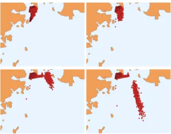
3.2 Met.no OD3D simulations
Fig. 5. Observations of the spreading of oil after the full city incident. All records regardless of amount of oil are included. Oil was also observed at Risør (23 km southwest of Jomfruland just outside the map) and Ruaker, near Grimstad (about 75 km southwest of Jomfruland).
Fig. 6. Contrast enhanced Envisat ASAR image on 4 August af-ter the “Full City” accident, superimposed geolocated aerial pho-tos from NCA. Courtesies; Press release as of 4 August 2009 from Nansen Environmental and Remote Sensing Center, Bergen, Nor-way. Envisat ASAR; © ESA. Aerial photos: www.kystverket.no.
model system does not describe the fine details in the topog-raphy). The wind changes direction from southwest wind to a more northern one after a few hours and the drift direction changes from north-northeast to almost southwards. Accord-ingly, 12 h after the accident the oil comes very close to the
shore on the other side of the fjord (i.e., the peninsula east of the accident site) but in this simulation the oil does not touch the coastline. Observations show that oil actually beached on this shoreline, and also on the shore on the peninsula east of the accident site. In previous studies it was apparent that the OD3D shows less dispersion (i.e., the numerical description of horizontal dispersion is perhaps too weak) than other sim-ilar models, and this may be one reason why particles do not beach over a large area as seen in observations. Another rea-son may be that currents are not accurate for this area for this period. We simply state that the met.no model system does not describe (i) the large beaching in the vicinity of the acci-dent site, and (ii) the advection of oil particles east-northeast during these conditions and that this is in conflict with ob-servations. This will be further discussed in the results and discussion section.
After 15 h the wave field and thus also the Stokes drift de-clines rapidly and the oil moves essentially with the ocean currents. The oil moves out from the coastal area and gets caught up by the coastal current at some distance from land. Here we find a rapid transport of particles southwards. This is further highlighted in Fig. 8. The oil spreads quickly south-westwards during the following 12 h. At model hour 20–30 the wind increases in strength and starts to blow toward the Norwegian coast. The oil starts to drift toward the coast and hits the coast over a large area around model hour 36 (Fig. 8). The dates of oil arrival to the coast given by the coastal au-thorities only give information about the days of detection
Fig. 7. First 24 h of the OD3D simulation with Skagerrak 1.5 km forcing (i.e. the oil 6, 12, 18, and 24 h after the accident). The red dots represent oil particles. The particles left behind very close to the land mask represent beached oil.
but it appears that the oil hit a large portion of the coast southwest of the accident site on 1–2 August, and we con-clude that the simulation is accurate for oil beaching in these areas. There were observations of oil further to the south and this is also described by the model; notably, the model only predicts minor beaching after 2 August.
Figure 8 also shows simulations based on the Nordic 4 km model (blue dots); it should be noted that the 4 km model is the only option for the present 24-7 operational oil drift model service. Due to the poor representation of the coast in this setup of the oil drift model, the oil drift has to be started at a location out in the Skagerrak. The oil particles are re-leased directly into the southward going coastal current and this model simulation has a much stronger south-westward drift along the coast than the 1.5 km model. Another peculiar feature of the 4 km model run is that the oil particles beach on the coastline of the 4 km grid (i.e., one half grid-point out from the coast due to the finite difference scheme for advec-tion). We conclude that within this setup of the model, the oil drift simulation based on the 4 km model do not describe observations particularly well. It is possible to improve the performance of the model by interpolating the ocean fields to a finer grid (which reduces the problems with the advec-tion scheme) but it is likely that the final simulaadvec-tions will not describe observations in the same detail as the model runs based on the 1.5 km model.
3.3 BSH oil drift simulation
The oil drift simulation by BSH using wind forecasts of the DWD is shown in Fig. 9. The oil particles initially move north-eastwards. Within the first 24 h some particles beach at the coast both north and northeast of the accident site. This
agrees well with observations although it is likely that the particles move slightly too slowly in this model simulation as compared to observations; furthermore, the model does not predict the extent of the beaching east of the accident site. The oil particles start to move southwards after 30–36 h reaching the coast west and southwest of the accident site af-ter 2 days. Afaf-ter 3 days, all the particles are beached at the coast over a distance of approximately 45 km. The beaching of particles takes place at the boundaries of grid cells having a resolution of 5 km in this area. As the observations show more beaching over a larger area, the BSH oil drift model un-derestimates the southward drift of oil. In spite of the rather coarse resolution in the Skagerrak area the main characteris-tics of the oil spill are well described within the model.
Compared to the 1.5 km met.no model, the BSH model computes weaker south-westward coastal current causing also slower drift velocities. Additionally, the slowness of the oil particles drift in the model is most likely due to the fact that the particles remain close to the coast at all times where current velocities are weak. It should be noted that even with this coarse resolution the model captures the oil beaching in a better way than the met.no 4km model in the sense that the oil gets to the north-east entrance of the fjord and the beach-ing times and locations match the observations in a better way.
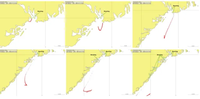
4 DAMSA oil drift simulation
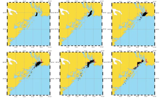
The oil drift simulation from the DAMSA setup of the Seatrack Web is shown in Fig. 10. Initially, we have a slow eastward drift of oil and there is some beaching north-east of the accident site. Approximately 10 h after the acci-dent the oil drift changes direction and becomes essentially out from the coast. There is some beaching on the southern tip of the peninsula east of the accident site (i.e., at Mølen), however, there is no beaching east of the tip of the penin-sula. The oil particles remain closely bunched at all times as a result of small dispersion in the model. It is likely that we would have larger amount of beaching if the numerical dispersion were increased in the model (which appears to be very small, as compared to OD3D and BSH model, given that all particles are well collected in a streak).
Fig. 8.The OD3D oil drift simulations using two different ocean models: red is for a 1.5 km model and blue is for a 4 km model. The figure shows the output 6, 12, 24, 36, 48, 60 h after the initial release of oil. Note that the 4 km (blue) model oil particles are beached well out into the sea due to low resolution: This model simulation also had to be initiated well out into the sea.
Fig. 10.The Seatrack Web oil drift simulation performed by DAMSA. The figures show the output 6, 12, 24, 36, 48, 60 h after the initial release of oil.
Fig. 11.Positions of the beaching of oil in the simulations presented in this study. The figure represents the oil 72 h after the initial release of oil.
5 Discussion and conclusions
5.1 Accuracy of the simulations
As stated earlier, the observed timing and amount of oil beaching in the “Full City” accident could be more precise. However, there are nevertheless some clear conclusions on the oil spill movements: (i) the coastal area northeast of the grounding site was immediately hit with large amounts of oil, (ii) the area east of the accident (up to 1 km east of the acci-dent site) was polluted by the oil spill, (iii) the area southwest of the grounding site (up to 60 km from the site of the acci-dent) was also hit by oil, and it appears that the beaching in this area took place about 1–2 days after the accident. This scenario is well reproduced in the model runs although there are some glitches.
5.2 Beaching of oil
5.2.1 First 24 h
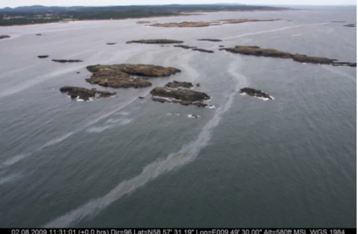
Fig. 12. Example of oil that is advected through a very complex topography. (Photo: NCA).
inter-comparison studies reveals that OD3D has less disper-sion than e.g., Meteo-France oil drift model (Brostr¨om et al., 2010). Releasing more particles and increasing the disper-sion rates in OD3D and Seatrack Web would probably give more realistic beaching in vicinity of the accident site.
Observations tell us that there was also some beaching on shores that are located up to 10 km east of the accident site. This is not captured in any of the models and requires some analysis. We have stated that there was a strong wind blowing along the coast, if this wind blew long enough there would be an Ekman transport out from the coast and there would be some upwelling of deep denser water along the coast. Accordingly, general theoretical arguments indicate that this may trigger a narrow coastal current in the direc-tion of the wind (Gill, 1982; Pedlosky, 1987). The width of the coastal current is given by the internal radius of deforma-tion (or internal Rossby radius),R=√gh01ρ/ρ0/f where gis gravity,1ρ is the density difference between the upper layer and the lower layer,ρ0is the reference density, andh0 is the thickness of the upper layer. Usingf=1.2·10−4 s−1, h0=10 m,ρ0=1000 kg m−3, and1ρ= 2 kg m−3(say 5◦C and 1 psu difference between upper and lower layer) the inter-nal radius of deformation is 3.7 km. It is clear that the low resolution models (for this particular area) used by met.no (4 km in the standard model), 5 km in the BSH model, and 5 km in DAMSA/SMHI model cannot describe the width and strength (which is coupled to the width) of the wind-driven coastal jet. In principle, the 1.5 km model could produce a solution that resembles this coastal jet; however, in the area around the grounding site the coastline is very complex and it is likely that even this model cannot describe a narrow strong current particularly well. More detailed studies are needed before we can make conclusive arguments about the exis-tence and strength of a north-eastward coastal jet driven by the wind, and if this is the main explanation of the eastward drift of oil in the “Full City” accident. Wave induced currents
that are not included in the present model system could also provide an explanation for the observed oil drift.
5.2.2 Oil drift between 24–72 h
After the initial north-eastwards movement of oil the wind changed direction and became directed out from the coast. OD3D and Seatrack Web predicted that oil particles moved out from the coast and well into the coastal current outside the Norwegian coast, while BSHdmod.L had some move-ment out from the coast but not as distinct as in the other two models. Accordingly, in OD3D and Seatrack Web the oil spill starts to move south-westwards rapidly when reaching the coastal current. The oil particles in Seatrack Web reach the southern tip of Norway by 3 August; OD3D runs based on the 4 km ocean model show a similar development while the run based on the 1.5 km model is somewhat slower. The oil particles in the BSHdmod.L never reach out in the coastal current and stay closer to the accident site than the particles in the OD3D and Seatrack Web.
After 40–48 h the wind changes direction toward the coast. The models respond by moving particles closer to the coast and there is significant beaching of oil particles southwest of the accident site in all models. There were many obser-vations of oil spill southwest of the grounding site about 1– 2 days after the accident and we concluded that all models give an accurate description of this feature, although it is still somewhat unclear if the magnitude of beaching is correct. Notably, there are some differences between the models:
– BSHdmod.L has beaching relatively close to the acci-dent site, and it takes place on 2 August (approximately at midday)
– The oil particles in OD3D using the 1.5 km model reach about 60 km southwest from the accident site and has beaching over a very large area at the same time (es-sentially 32 h after the accident, i.e., at 2 August at about 06:00). The simulation based on the 4 km grid has beaching at about the same time but over a much larger area.
– Seatrack Web predicts that there will be beaching of par-ticles after about 48 h, and the beaching takes place over a wide area almost down to the southern tip of Norway. There are uncertainties regarding the beaching of oil south-west of the accident site but it appears that OD3D describes the beaching in this area correctly.
unlikely that large amounts of oil moved this far south along the coast. However, there were scattered observations along the coast giving some credibility to the simulations.
The three different modeling systems use very different formulations for forcing and oil drift (see Table 1), neverthe-less, the results of the model are quite similar. The reason is most likely that different formulations are in practice rather similar. It is likely that the atmospheric forcing is quite sim-ilar given that the data that are used to force the atmospheric models are shared among the different meteorological insti-tutes. The “wave” factor in the oil drift can either be de-scribed according to Stokes drift or as say 2–3 % of the wind speed, this latter follows from an assumption that the wave field is entirely governed by the wind speed. The main dif-ference is probably in the ocean model, although the ocean models based on similar dynamics they will differ in the de-tails on the placement and strength of eddies and the dynam-ics in near shore areas.
5.2.3 Land masks
We see large differences in the way coastlines are treated. In OD3D and BSH model the oil is beached on the side of the numerical grid while the oil is beached on the land mask in the Seatrack Web. In the OD3D model, the main part of the particles based on the 4 km model is beached well out in the ocean, this is mainly due to an unfortunate numeri-cal scheme that does not allow for advection of particles in the one half grid-point closest to the coast. The situation becomes much better with the 1.5 km model than the 4 km model. The beaching in the BSH model is better described although it is obvious that particles are beached on the sides of grid cell, and that these do not represent the coastline very accurately. Seatrack Web follows another strategy and uses high-resolution coastlines to track beaching.
In fact, although the beaching is a very important parame-ter in most models the physics of beaching is not adequately described in the models. If there were no direct wind drift acting on the particles, beaching would not occur in an ocean model with accurate numerical schemes simply because no water particles can come in contact with the model’s imper-meable walls. Consequently, we conclude that, in the mod-els, beaching is the result of (i) direct drift by wind or waves, (ii) numerical dispersion of particles, or (iii) inaccurate nu-merical schemes. In reality, the beaching is probably very complex and depends on processes with strong vertical shear due to (i) wind drift and (ii) Stokes drift, which are not de-scribed in classical circulation models. The representation of beaching in a complex geometry and the amount of oil that passes through is a challenge for the future, but is much needed for more accurate forecasting of oil spill in areas with complex geometry (see e.g., Fig. 12).
Acknowledgements. This work has been sponsored by EC through the project ECOOP, and the Norwegian Research council through the project OilWave 207541. We would also like to thank Bruce Hackett for comments and careful reading of the manuscript.
Edited by: E. Stanev
References
Ardhuin, F., Mari´e, L., Rascale, N., and Forget, P.: Observation and estimation of Lagrangian, Stokes and Eulerian currents induced by wind and waves at the sea surface, J. Phys. Oceanogr., 39, 2820–2838, 2009.
Blumberg, A. F. and Mellor, G. L.: A description of a three-dimensional coastal ocean circulation model, in: Three-Dimensional Coastal Ocean Models, edited by: Heaps, N. S., AGU Coastal and Estuarine Series, American Geophysical Union, Washington D.C., 1987.
Brostr¨om, G., Carrasco, A., Hackett, B., and Sætra, Ø.: Us-ing ECMWF products in global marine forecastUs-ing services, ECMWF newsletter, 118, 16–20, 2009.
Brostr¨om, G., Carrasco, A., Daniel, P., Hackett, B., and Paradis, D.: Comparison of two oil drift models and different ocean forc-ing: With application to Mediterranean drifter trajectories and North Sea oil spill, in: Coastal to global operational oceanogra-phy: Achievements and challanges, Eurogoos publication no. 28, 5th Eurogoos conference, Exeter, 2010, 260–266, 2010. Castanedo, S., Medina, R., Losada, I. J., Vidal, C., M´endez, F.
J., Osorio, A., Juanes, J. A., and Puente, A.: The Prestige Oil Spill in Cantabria (Bay of Biscay). Part I: Operational Fore-casting System for Quick Response, Risk Assessment, and Pro-tection of Natural Resources, J. Coast. Res., 22, 1474–1489, doi:10.2112/04-0364.1, 2006.
Cavaleri, L., Alves, J.-H. G. M., Ardhuin, F., Babanin, A., Banner, M., Belibassakis, K., Benoit, M., Donelan, M., Groeneweg, J., Herbers, T. H. C., Hwang, P., Janssen, P. A. E. M., Janssen, T., Lavrenov, I. V., Magne, R., Monbaliu, J., Onorato, M., Polnikov, V., Resio, D., Rogers, W. E., Sheremet, A., McKee Smith, J., Tolman, H. L., van Vledder, G., Wolf, J., and Young, I.: Wave modelling – The state of the art, Prog. Oceanogr., 75, 603–674, 2007.
Coppini, G., De Dominicis, M., Zodiatis, G., Lardner, R., Pinardi, N., Santoleri, R., Colella, S., Bignami, F., Hayes, D. R., Soloviev, D., Georgiou, G., and Kallos, G.: Hindcast of oil-spill pollution during the Lebanon crisis in the eastern Mediterranean, Mar. Pol-lut. Bull., 62, 140–153, 2011.
Daniel, P., Josse, P., and Dandin, P.: Further improvement of drift forecast at sea based on operational oceanography systems, Coastal Engineering VII, Modelling, Measurements, Engineer-ing and Management of Seas and Coastal Regions, Algarve, Por-tugal, 13–22, 2005.
Dick, S. and M¨uller-Navarra, S. H.: An Operational Oil Spill Model for the North Sea and the Baltic – Model features and appli-cations, Third RD Forum on High-Density Oil Spill Response, Brest, IMO 61–70, 2002.
Dick, S., Kleine, E., and Janssen, F.: A new operational circulation model for the North Sea and the Baltic using a novel vertical co-ordinate - setup and first results, Fifth International Conference on EuroGOOS, Eurogoos publication, no. 28, Exeter, UK, 225– 231, 2010.
Diez, S., Jover, E., Bayona, J. M., and Albaig´es, J.: Prestige Oil spill. II. Fate of a heavy oil in the marine environment, Environ. Sci. Technol., 41, 3075–3082, 2007.
Engedahl, H.: Implementation of the Princeton Ocean Model (POM/ECOM3D) at the Norwegian Meteorological Institute, Norwegian Meteorological Institute, Oslo, Norway5, 40, 1995. French-McCay, D. P.: Oil spill impact modeling: Development and
validation, Environ. Toxicol. Chem., 23, 2441–2456, 2004. Gill, A. E.: Atmosphere-Ocean Dynamics, Academic Press, Inc.,
London, 662 pp., 1982.
Komen, G. J., Cavaleri, L., Donelan, M., Hasselmann, K., Hassel-mann, S., and Janssen, P. A. E. M.: Dynamics and modelling of ocean waves, Cambridge University Press, Cambridge, 532 pp., 1994.
Lorentsen, S.-H., Bakken, V., Christensen-Dalsgaard, S., Follestad, A., Røv, N., and Winnem, A.: Akutt skadeomfang og herkomst for sjøfugl etter MV Full City-forliset., Norsk Institutt for Natur-forskning, Trondheim, Norway, 44, 2010.
Martinsen, E. A., Melsom, A., Sveen, V., Grong, E., Reistad, M., Halvorsen, N., Johansen, Ø., and Skognes, K.: The operational oil drift system at DNMI., Norwegian Meteorological Institute, Oslo, Norway, 125, 52, 1994.
Mellor, G. L. and Yamada, T.: Development of turbulence clo-sure model for geophysical fluid problems, Rev. Geophys. Space Phys., 20, 851–875, 1982.
Melsom, A.: A review of the theory of turbulence closure due to Mellor and Yamada, and its implementation in the Princeton Ocean Model, Norwegian Meteorological Institute, Oslo, Nor-way, 38, 47, 1996.
Olsen, E.: Miljøundersøgelser i forbindelse med forliset av M/S “Full City”, Institute of Marine research, Bergen, Norway, 28, 2009.
Pedlosky, J.: Geophysical fluid dynamics, Springer-Verlag, New York, 710 pp., 1987.
Phillips, O. M.: The dynamics of the upper ocean, Cambridge Uni-versity Press, Cambridge, 336 pp., 1977.
Proctor, R., Flather, R. A., and Elliott, A. J.: Modelling tides and surface drift in the Arabian Gulf—application to the Gulf oil spill, Cont. Shelf Res., 14, 531–545, 1994.
Reed, M., Johansen, Ø., Brandvik, P. J., Daling, P. S., Lewis, A., Fiocco, R., Mackay, D., and Prentkim, R.: Oil spill modelling towards the close of the 20th century: Overview of the state of the art, Spill Sci. Technol. B, 5, 3–16, 1999.
Røed, L. P. and Debernard, J.: Description of an integrated flux and sea-ice model suitable for coupling to an ocean and atmosphere model, Norwegian Meteorological Institute, POBox 43 Blindern, 0313 Oslo, Norway, 51, 2004.
Soomere, T., Viikm¨ae, B., Delpeche, N., and Myrberg, K.: Toward identification of areas of reduced risk in the Gulf of Finland, the Baltic Sea, P. Est. Acad. Sci., 59, 156–165, 2010.
Soomere, T., Berezovski, M., Quak, E., and Viikm¨ae, B.: Modelling environmentally friendly fairways using Lagrangian trajectories: a case study for the Gulf of Finland, the Baltic Sea, Ocean Mod-ell., 60, 1–12, doi:10.1007/s10236-10011-10439-y, 2011. Tijm, A. B. C. and Lenderink, G.: Characteristics of CBR and
STRACO Hirlam Newsletter, 43, 10 pp., 2003.
Und´en, P., Rontu, L., J¨arvinen, H., Lynch, P., Calvo, J., Cats, G., Cuxart, J., Eerola, K., Fortelius, C., Garcia-Moya, J., Jones, C., Lenderlink, G., McDonald, A., McGrath, R., Navascues, B., Nielsen, N., Odegaard, V., Rodriguez, E., Rummukainen, M., R¨o¨om, R., Sattler, K., Sass, B., Savij¨arvi, H., Schreur, B., Sigg, R., The, H., and Tijm, A.: HIRLAM-5 Scientific Documentation, Swedish Meteorological and Hydrological Institute, Norrk¨oping, Sweden., 2002.
Wanga, S. D., Shena, Y. M., Guob, Y. K., and Tanga, J.: Three-dimensional numerical simulation for transport of oil spills in seas, Ocean Eng., 35, 503–510, 2008.
Venkatesh, S. and Murty, T. S.: Numerical simulations of the move-ment of that 1991 oil spills in the Arabian Gulf, Water, Air, Soil Pollut., 74, 211–234, 1994.
Wettre, C., Johansen, Ø., and Skognes, K.: Development of a 3-dimensional oil drift model at DNMI, Norwegian Meteorological Institute, Oslo, Norway,, 50, 2001.