Research Article
Morphological feature selection and neural classiication
for electronic components
Dionysios Lefkaditis and Georgios Tsirigotis* Kavala Institute of Technology, 65404, St.Lucas, Kavala, Greece.
Received 21 September 2009; Revised 4 November 2009; Accepted 18 November 2009
Abstract
This paper presents the development procedure of the feature extraction and classiication module of an intelligent sorting system for electronic components. This system was designed as a prototype to recognise six types of electronic components for the needs of the educational electronics laboratories of the Kavala Institute of Technology. A list of features that describe the morphology of the outline of the components was extracted from the images. Two feature selection strategies were ex -amined for the production of a powerful yet concise feature vector. These were correlation analysis and an implementation of support vector machines. Moreover, two types of neural classiiers were considered. The multilayer perceptron trained with the back-propagation algorithm and the radial basis function network trained with the K-means method. The best re -sults were obtained with the combination of SVMs with MLPs, which successfully recognised 92.3% of the cases.
Keywords: Recognition, Neural Network, Classiication.
Journal of Engineering Science and Technology Review 2 (1) (2009)151-156
Technology Review
www.jestr.org
This paper gives an account of the construction of an intelligent sorting system for electronic components. Speciic focus is given on the comparison of two feature selection methods used to optimise the morphological feature vector. Correlation analysis and support vector machines were considered as they represent two very dif-ferent approaches for feature selection. The performance of these methods was measured through the successful recognition rates of two neural classiiers, the multilayer perceptron and the radial basis function network. The best performing combination of methods was
then proposed as the classiication module of the sorting system. Correlation analysis was utilised to discover any underlying relationships between the features, in essence to ind out if they refer to the same property of the sample’s outline. Therefore, un-wanted repetitions of information were discarded, thus the feature vector was shrunk and simpliied with minimum loss of its descrip-tive ability.
Support vector machines (SVMs) were examined as an alter-native technique for feature selection. Here, SVMs were set to per-form a supervised classiication task on the data. The focus was not to optimise the classiication performance but to quantify the dis-crimination ability of the features and sort them on this basis. The sorting criterion was the squared weight of each variable deined by the support vectors.
The multilayer perceptron class of neural networks consists of
multiple layers of computational units, interconnected in a feed-forward way. Each neuron in one layer has directed connections to the neurons of the subsequent layer and applies a sigmoid function as an activation function [9]. These networks were trained using the supervised back-propagation algorithm [3].
A radial basis function (RBF) is a function, whose value is
governed by the distance from a centre. RBFs have been applied in the area of neural networks, where they may be used as a replace-ment for the sigmoidal hidden layer transfer characteristic in multi-layer perceptrons. The RBF chosen is usually a Gaussian distribu-tion funcdistribu-tion [3]. The training of these networks was to calculate the coordinates of the Gaussian centres by the unsupervised K-means clustering method [5].
2. Materials and methods
2.1 Image acquisition and processing
The acquisition of images took place at the laboratories of the Fish-eries Research Institute at Nea Peramos, Kavala, Greece. The in-stitute kindly provided all the necessary equipment and laboratory space for the needs of this study.
The device characteristics that were desired for this applica-tion were the adequate image resoluapplica-tion of the sensor, good quality optics, the space available between the objective lens and the sam-ple, the adaptability to various lighting techniques and the speed
* E-mail address: [email protected]
ISSN: 1791-2377 © 2009 Kavala Institute of Technology. All rights reserved.
of operation. After the examination of several available devices the one that offered the most attractive combination of the above was a high precision desktop photographic system with a standalone con -trol unit made by Nikon.
The use of back illumination was found to eficiently deal with problems such as the presence of shadows and the relections of me -tallic surfaces. The sample was situated in between the light source and the image sensor. In this manner, the sample appeared to be dark in a bright background. Another advantage of this technique was that the foreground-to-background contrast was very high. The disadvantage of decreased colour information was not important for the speciic application.
A Leica stereoscopic microscope stage in conjunction with a Leica L2 ibre optic light source and a transparent sample holder was used to achieve the back-illumination lighting. A piece of A4 paper was placed between the sample and the sample holder to dif-fuse the light and create an evenly illuminated background. This technique gave excellent results and minimised the need for ad -vanced image-processing algorithms to extract the sample outlines. The image acquisition setup can be seen in igure 1.
In this study, custom code was developed to automatically per-form the image processing and feature extraction. The open-source and Java-based application ImageJ was used as a platform for this task [1]. The images were scaled and cropped, and the colour infor -mation was discarded by converting the images from 24bit colour to 8bit greyscale to reduce the unnecessary volume of data and speed up the processing. Image segmentation was performed using the “Minimum Auto Threshold” algorithm [11]. The mathematical mor -phology algorithm “closing” was applied to ix any broken lines
as a result of local miscalculation of the threshold limit [13]. This ensured the reliable production of image measurements for the ex -traction of the features.
2.2 Extraction of morphological features
Feature extraction is performed as a way to reduce the dimensional -ity of the data produced by the image sensor. In the computer vision ield, each pixel represents one data dimension. The images used in this study provided data of 200340 dimensions as the images used
were 477x420 pixels. It is impractical to feed data of such high di -mensionality into a classiier. A long list of candidate features was calculated in order to form a powerful input vector for the neural classiication module of the system. The features attempted to de -scribe the morphology of the outline shape of the electronic com -ponents. Once extracted and optimised, the vector would be used to train and validate the classiier. The list of candidate features con -tained:
• Area.
This is calculated as the sum of pixels that are enclosed within the boundaries of the sample. It is then converted in calibrated units, such as μm2 to enable direct comparison among sample images that are not acquired using the same lens set-up on the stereoscope. It may be useful to give a measure of absolute size. • Perimeter.
This is calculated as the sum of the pixels that form the boundary of the sample. It is also converted in calibrated units (μm) ac -cording to the lens set-up of the stereoscope. It offers a measure of size as well as a measure of outline roughness.
• Maximum Feret’s diameter.
This is deined as the greatest distance possible between any two points along the boundary of the sample or the greatest distance between two vertical lines tangential to the ends of the particle [1]. It is useful in conjunction with magniication data from the stereoscope to give a measure of actual size scale of the sample. • Circularity.
A simple shape factor based on the projected area of the sample and the overall perimeter of the projection according to:
(1)
where A is the area and P is the perimeter of the sample.
Values range from 1, for a perfect circle, to 0 for a line. It is useful to give an impression of elongation as well as roughness of the sample’s shape. Other signiicant characteristics of this feature are that it is invariant to scale, translation and rotation [4].
• Solidity.
It is the ratio of the area of the sample (A) over the area of its convex hull (AConvexHull) [6]. The formula for solidity is:
(2)
• R factor.
The R factor measures the perimeter of the convex hull of the sample over its maximum Feret’s diameter [6]. R factor is given by:
(3)
• MBR aspect ratio.
This is the ratio of the sides of the “minimum bounding rec -tangle” (MBR) that includes the sample. The minimum bounding rectangle, also known as “bounding box”, is an expression of the
maximum extents of a 2-dimensional object (e.g. point, line, poly-gon) within its 2-D (x,y) coordinate system, in other words min(x), max(x), min(y), max(y) [7]. It may be useful to give a measure of the elongation of the samples. The formula for aspect ratio is:
(4)
• Convexity.
It is the ratio of the perimeter of the convex hull of the sample (PconvexHull) over the actual perimeter of the sample (P). For planar
objects, the convex hull may be easily visualized by imagining an
elastic band stretched open to encompass the given object; when released, it will assume the shape of the required convex hull [8]. The formula for convexity is:
(5)
• Concavity.
This is the subtraction of the area of the sample (A) from the area covered by its convex hull (AConvexHull) [6]. The formula used
for concavity is:
(6)
• Rectangularity.
This is the ratio of the area of the sample over the area of its MBR [10]. It approaches 0 for cross-like objects, 0.5 for squares, π/4 for circles and 1 for long rectangles [6]. The formula used for rectangularity is:
(7)
• Feret’s aspect ratio
This is the ratio of the maximum Feret’s diameter over the max -imum diameter of the object which is perpendicular to the one of Feret’s, in other words the breadth of the object. It is given by:
(8)
• Roundness.
It is given by the area of the sample over the square of its maxi-mum Feret’s diameter [6]. The formula for roundness is:
(9)
• Compactness
This feature also associates the area of the sample over its maxi-mum Feret’s diameter. The formula to calculate it is:
(10)
Area, perimeter and maximum Feret’s diameter were extract-ed to enable the calculation of the rest of the features and were not included in the feature vector.
2.3 Feature selection
The extraction of the 13 features mentioned above produced a mul-tidimensional set of data. The exploration of the data set can give a valuable insight of the expected behaviour of the end system and therefore assist further improvement of its performance [10]. This knowledge can be gained by inding out the internal relationships between the features and the quantiication of their descriptive power.
The feature selection and the classiication tasks of this study were performed with the widely respected open-source software package WEKA [14].
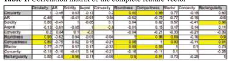
In multidimensional data sets, correlation analysis is comput-ed by calculating the Pearson coeficient between every
combina-tion of features. The resulting values were then arranged in a table format called correlation matrix. In the event that the value of the coeficient was higher than ±0.85, the correlation was considered too high and one of the two features was excluded from the feature vector.
The use of the correlation matrix simpliied the detection of high correlating features and the decision of which one should be excluded. Table 1 illustrates the correlation matrix:
In the correlation matrix, the values that lie above the limit are highlighted in yellow and the features considered for exclusion in grey. After the selection process six features remained in the optimised feature vector. These are shown in table 2:
Feature name
Feret's aspect ratio
Solidity MBR aspect ratio
Convexity R factor Concavity
A good example for illustrating the relationship between two high correlating features was “Roundness” and “Compactness”. A plot of their values against each other is presented in igure 2, which it is very close to a straight line as they are highly correlated: Table 1. Correlation matrix of the complete feature vector
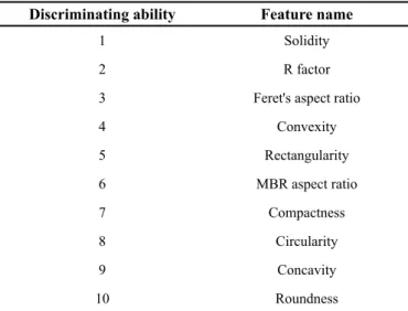
As mentioned before, SVMs were used as supervised alter-native feature selection technique to the unsupervised correlation analysis. After the classiication, features were sorted based on their discriminating ability. Table 3 presents the results of this tech-nique:
Discriminating ability Feature name
1 Solidity
2 R factor
3 Feret's aspect ratio
4 Convexity
5 Rectangularity
6 MBR aspect ratio
7 Compactness
8 Circularity
9 Concavity
10 Roundness
For direct comparison with correlation analysis the six most powerful features were selected. It is worth noting that the two op -timised feature vectors are very similar to each other. 5 out of the 6 features selected were the same. SVMs selected rectangularity in -stead of concavity that was selected by correlation analysis.
The actual performance of the optimised vectors was measured through the performance of classiication module of the system.
2.4 Classiier training and validation
In this study, two neural classiiers were considered that use very different training approaches. The multilayer perceptrons (MLPs) are trained with the supervised back-propagation algorithm. The radial basis function networks (RBFNs) use the K-means cluster -ing method to deine the centres of their Gaussian functions. The K-means is a well-known unsupervised technique.
Initially, these networks were trained with the full 10-element feature vector so as to set it as the benchmark to which the opti-mised feature vector would be compared. Therefore, the classiier
validation served two purposes, the identiication of the most pow -erful feature selection technique and the determination of the most suitable classiier for this application.
Generally in the classiication neural networks, it is common practice to use the number of elements of the feature vector as the number of neurons of the input layer and the number of neurons of the output layer to be the number of classes of the data. In this ap-plication for the MLP, the number of neurons was found in a trial and error manner. However, the approach that gave the best results was to use the half of the sum of the rest of the nodes of the network as the number of hidden nodes. For example, in the case of the full feature vector, there were 10 input and 6 output nodes that made 8 nodes in the hidden layer. Moreover, the best learning rate and the momentum factor of the back-propagation training were found to be 0.8 and 0.3 respectively. The networks were trained for 1000 cycles as longer training did not provide lower error rates. The data, consisting of 87 sets in total, was split in 70% for training and 30% for validation.
After the training sessions, the classiier evaluation yielded an overall performance of 92.3%. The various classes gave differing degrees of successful recognitions that can be described by two met -rics. True Positive (TP) rate is the actual rate of successful recogni -tions and False Positive rate (FP) shows the percentage of mistak -enly classiied cases per class. Table 4 presents the detailed results.
The class Elcap refers to electrolytic capacitors, Cercap to square and round ceramic capacitors, Res to resistors, Trans to tran-sistors and PowTrans to power trantran-sistors.
Class TP FP
Elcap 0,857 0,053
Cercap sq 0,833 0
Cercap rd 1 0
Res 1 0
Trans 1 0
PowTrans 1 0,045
An alternative presentation method of these results is the con-tingency table, where it the misclassiication are shown more clear -ly. The diagonal of the table depicts the true successful recognitions. The contingency table is table 5.
Classes classiied as...
Elcap Cer-cap sq
Cer-cap rd Res Trans Pow
Trans Classes
6 0 0 0 0 1 Elcap
0 5 1 0 0 0 Cercap sq
0 0 1 0 0 0 Cercap rd
0 0 0 5 0 0 Res
0 0 0 0 3 0 Trans
0 0 0 0 0 4 PowTrans
The table below suggests that the overall classiication rate was very high. However, the electrolytic capacitors can be confused with power transistors and the square ceramic capacitors as round
Figure 2. Plot of Roundness against Compactness showing their high correlation
Table 3. Features sorted by their discriminating ability using SVMs
Table 4. Detailed MLP classiication performance per data class
ones. Considering the nature of feature within the input vector, it can be realised that these classes have indeed very similar shape and outline properties.
For the RBFNs, the number of Gaussian functions needs to be far greater than the expected data clusters in the feature space, so as for the network to able to map the data with enough resolution. Here they were trained with 30 nodes in their hidden layer as higher number of Gaussians did not offer better results.
As it was expected the unsupervised RBFNs did not match the performance of the MLPs. They gave an overall successful recogni -tions rate of 65.4%. Therefore, they are not recommended for this application.
The performance of the MLP networks trained with the op-timised feature vectors was very high. For both the optimisation methods it matched the overall successful recognitions rate of 92.3% and the per class rates. This shows that both of the meth -ods achieved to discard only repetitive and unneeded information. Therefore, there can be more than one optimised feature vectors for a speciic application.
The RBFNs also gave interesting results when trained with the optimised vectors. The correlation analysis vector offered an in-crease of 3.84% to the overall successful recognitions rate, making it 69.2%. This was probably because the unsupervised networks are very prone to confusing and repetitive data.
Training the RBFNs with a supervised feature selection tech-nique dramatically improved their performance. They achieved to give 84.6% successful recognitions rate, an increase of 19.2%. Therefore, the SVMs offer a far more powerful feature vector. This method is based on actual supervised classiication, which sorts the features according to their real descriptive abilities and it is not de -pendant on the discovery of underlying subjective relationships be-tween the features. It is therefore, a matter of comparison bebe-tween a supervised and an unsupervised methodology on the same data set, where it is expected that the supervised one will be superior.
In order to examine whether a six element feature vector is the optimum size for this application, one more element was excluded from both the optimised vectors. The performance decreased for the MLPs and the RBFNs for both optimisation methods. It needs to be noted that SVMs gave a smaller performance decrease for both network types. This means that it is also more reliable than correla-tion analysis on the speciic applicacorrela-tion. Therefore, here it is the preferred method.
All the above results are presented graphically in igure 3 and documented in detail in table 6.
3. Conclusions
This paper presented a thorough account of the feature selection process and the development of the neural classiier a computer vision system for the recognition of electronic components.
Optimisation
Vector element number
none
Cor-relation analysis
SVM
10 92.31% 65.38% - - -
-6 - - 92.31% 69.23% 92.31% 84.62%
5 - - 84.62% 65.38% 88.46% 80.77%
Classiier MLP RBFN MLP RBFN MLP RBFN
The system was designed with the generic model of the modu -lar machine vision system by Awcock and Thomas [2] as a guide. The image acquisition equipment was a Nikon high precision desk -top photographic system with a standalone control unit as it offered high quality images, adaptability to various lighting techniques and speed of operation. The lighting technique used was back-illumi-nation so that the creation of shadows and relections of metallic surfaces can be avoided.
The processing of the images and the feature extraction re -quired were implemented as a custom ImageJ macro code. A list of 10 morphological features based on the outline of the samples was calculated to reduce the dimensionality of the image data.
Two types of neural classiiers were considered, the multilayer perceptrons (MLPs) and the radial basis function networks (RBFNs). These classiiers were initially trained with the full feature vector to act as a benchmark. Two feature vector optimisation methods were examined, correlation analysis and SVMs. Generally, the MLP clas -siiers performed much better than the unsupervised RBFNs. For the MLPs, both feature selection methods matched the performance given by the full feature vector. However, for the RBFNs, the SVMs presented a far better performance than with both the full and the correlation analysis optimised feature vector. They are better suited to this application because it is a supervised feature selection tech-nique on a supervised classiication problem. Therefore, the SVMs were considered as a more reliable feature selection method for the inal system even though it offers the same performance as with the other feature vectors for the chosen MLP classiier.
Training with a further reduced ive-element feature vector showed a decrease in performance for both MLPs and RBFNs. This proved that the vector size of six elements was indeed the right vec-tor size for this application.
As a inal conclusion, for the above reasons the combination of the SVM optimised six-element feature vector with the MLP neural networks was considered to give the most powerful clas-siication module for this computer vision system.
Figure 3. Concentrative graph of classiier performances
1. Abramoff, M. D., Magelhaes, P. J., Ram, S. J., 2004. “Image Processing with ImageJ”. Biophotonics International, volume 11, issue 7, pp. 36-42. 2. Awcock, G. J. & Thomas, R., 1995. Applied image processing, Hights
-town, NJ, USA: McGraw-Hill, Inc.
3. Bishop, C. M., 1995. Neural Networks for Pattern Recognition, Oxford,
UK: Oxford University Press.
4. Bouwman, A. M., Bosma, J. C., Vonk, P., Wesselingh, J. A. & Frijlink, H.W. (2004) Which shape factor (s) best describe granules. Powder Tech
-nology, 146 (1-2), pp.66-72.
5. Duda, R, Hart, P & Stork, D., 2001, Pattern classiication, Wiley New
York.
6. Eid, R. & Landini, G., 2006. Oral Epithelial Dysplasia: Can quantiiable morphological features help in the grading dilemma? In Luxembourg. 7. Glasbey, C. & Horgan, G., 1995. Image analysis for the biological sci
-ences, New York: Wiley.
8. Graham, R., 1972. An Eficient Algorithm for Determining the Convex
Hull of a Finite Planar Set. Information Processing Letters, 1(4), 132-133. 9. Haykin, S., 1998. Neural Networks: A Comprehensive Foundation, Pren
-tice Hall PTR Upper Saddle River, NJ, USA.
10. Lefkaditis, D., Awcock, G. J. & Howlett, R. J., 2006. Intelligent Optical Otolith Classiication for Species Recognition of Bony Fish. In Interna
-tional Conference on Knowledge-Based & Intelligent Information & En
-gineering Systems. Bournemouth, UK: Springer-Verlag, pp. 1226-1233. 11. Prewitt, J. & Mendelsohn, M., 1966. The analysis of cell images. Ann. NY
Acad. Sci, 128, 1035-1053.
12. Rosin, P. L., 2003. Measuring shape: ellipticity, rectangularity, and trian
-gularity. Machine Vision and Applications, 14(3), 172-184.
13. Serra, J., 1983. Image analysis and mathematical morphology. Academic Press, Inc. Orlando, FL, USA.
14. Witten, I and Frank, E, 2005. “Data Mining: Practical machine learning tools and techniques”, 2nd Edition, Morgan Kaufmann, San Francisco.