Automatic classification of green areas for
cartography purposes
Joel Augusto Joanaz D’Assunção Dias, [email protected]
Academia Militar, Lisbon Instituto Superior Técnico, Lisbon
Abstract — This paper exposes a study with the purpose of discriminating the different types of vegetation. One way to get information about the land is through cartography, where aerial photogrammetry is one of the most used techniques. The main objective of this study is the development of a tool capable of processing aerial photographs on the visible spectrum and for it to be able to discern and classify the different types of vegetation.
The adopted methodology comprises into three major steps: feature extraction, feature selection and image classification using two classifiers, K-Nearest Neighbors and Support Vector Machine. The first step extracts statistical features and features of texture, the second step implements a technique that allows the selection of the most relevant features and the last step is divided in the optimization of the classifiers input parameters and subsequent image classification.
It was not possible to use the eight classes pre-defined due to the similarity between some of them, which led to the merge of some, resulting in four new classes. The images were classified according the new classes and the performance of the two classifiers was compared. It was found that the best classifier is the Support Vector Machine using the function of kernel Radial Basis Function showing 89,8% of correct classifications. The influence of the feature selector was tested and it was concluded that it led to an average increase of 8,25% in the classifier’s performance. It was also concluded that the best results were achieved with 10 features for the K-Nearest Neighbors and with 20 features for the Support Vector Machine.
Keywords — Aerial photography, Classification, Feature Selector, Vegetation
I. INTRODUCTION
ne way to get terrain’s knowledge is through cartographic information, which sometimes can only be obtained through aerial photographs. This acquisition is held during flights, which, depending on camera’s specifications, allows to gather photos with information in the visible spectrum or multispectral. The
collected data allows the extraction of terrain’s features. The Centro de Informação Geoespacial do Exército (CIGeoE) is the entity, by excellence, responsible for cartographic production, in Portugal. They have teams with specialized photogramme-trists whose job is to interpret aerial photographs’ information in CIGeoE’s geographical data base.
The creation and implementation of algorithms capable of discriminate a plant cover is an area with a significant growth rate among the scientific community. There have already been developed many implementations that enable to control the borders, to identify different species of vegetation and to control the deforestation, through machine learning. This was a motivation factor to develop this paper.
The main objective of this paper is the development of a methodology that processes aerial photos, extracting relevant information that allows the discrimination of different types of vegetation through the application of automatic classifiers, with a reduced probability of error. Secondly, it is made a comparison of the overall accuracy between the implemented classifiers, as well as the influence that a feature selector method introduces on the results obtained.
II. BACKGROUND
Over the past decades, various classification methods have been improved to correspond with the various types of vegetation that are found [1].
Lewis et al [2] compares the cost-effectiveness of seven mapping approaches: one method based on aerial photography interpretation (API); two pixel-based image analysis (PBIA) methods and four geographic-based image analysis (GEOBIA) methods. Overall, accuracy ranged from 28% to 67% for the seven approaches. API approach presented the highest overall accuracy (67%) for the 1:25000 spatial scale map, and the PBIA approach applied to Landsat5 TM at 1:25000 demonstrated the lowest (28%). Regarding to the cost, the API revealed to be the most labor-intensive and expensive approach, though it got better results, while the PBIA was the least expensive approach, however it got the lowest results.
Laliberte et al [4] proposes methods based on the object-based images analysis (OBIA) in order to classify the different types of vegetation in arid regions of the south west of the United States of America, given by aerial images
multispectral (visible and near infrared) with a dimension of 13824x7680 pixels; each pixel representing 4 centimeters. The process begins with a segmentation of the image in homogeneous areas using three parameters (scale, color and shape), each with a weight between 0 and 1. Four features are extracted: intensity value of the pixels, Normalized Difference Vegetation Index (NDVI), average and ratio of 3 bands. Subsequently, two classifiers are used, the rule-based that uses two features: intensity value of pixels and NDVI, and the K-Nearest Neighbors (KNN) classifier that uses 3 features: NDVI, average and ratio of 3 bands.
Zhengrong Li et al [4] describes a method which consists in the use of a descriptor resulting from the merger of color and texture with the purpose of classifying the different species of trees. It develops an automatic segmentation to detect and delineate the trees crowns by eliminating the rest, extracting the Uniform Local Binary Patterns (ULBP). Subsequently, it applies the Principal Component Analysis (PCA) to find non linear relations between features of color and texture that were extracted. After that, maximum verisimilitude is used to estimate what are the best set of features that should be used in Support Vector Machine (SVM) classifier. That are used in high-resolution aerial images, with pixel size of 15 centimeters. To be able to assess this method the authors apply the same method, but with separate features. From here they get a classification’s accuracy of 80.2% for color and 71.1% for texture. On the other hand, the fusion method obtains an accuracy of 83,5%, which confirms that the best results are achieved when using fusion.
Chapman et al [5] suggests a solution for the vegetation classification using aerial orthorectified multispectral photographs with a spatial resolution of 5 meters. These images are removed from a set of features that are used on a method that consists in regression trees and classification allowing you to define the rules. To calculate these rules, we resort to a recursive method that makes the partition in the binary data, until there are obtained homogeneous regions, also designated by us, each one with a class information. Seven classes of vegetation are defined and the classifier Random Forest is applied, so as can be performed a hierarchical classification. This method allowed to obtain an accuracy of 97% in correct classifications.
U. Bradter et al [1] presents a study about the Yorkshire Dales National Park, in England, on vegetation classification, that uses aerial orthorectified images in the visible band with a spatial resolution of 5 meters. The aim was to investigate the influence of using variables such as physical, elevation, inclination and types of soil, in the effectiveness of ratings. Three features of images are extracted: the average of the pixels’ values’ intensity in each band, the ratio between the average values calculated earlier and a measure of heterogeneity of spectral intensity. These features are introduced in the Random Forest classifier, where it gets an accuracy between 87% and 92%.
Minho et al [6] uses an GEOBIA approach in aerial images with 30 cm of spatial resolution to classify swamps in three classes: vegetation, channel and mud. It investigates three classification problems associated with the scale used in the segmentation: the comparison between the use of
GEOBIA with one or several scales, the benefit to incorporate information on texture from Gray-Level Co-Occurrence Matrix (GLCM) and, lastly, the effect of the use of levels of quantization in GLCM. He concluded that for the first problem, the multi-scale approach exceeds the approach with only a scale, obtaining an overall accuracy of 82% against 76% obtained with one scale. The addition of texture improves the spectral discrimination and leads to a classification’s accuracy’s increase from 3% to 12%, when included in the multi-scale approach. Regarding the third problem, it was concluded that the use of only two levels of quantization induces in obtaining better ratings.
III. METHODS
This section will describe the methodology used in this study to discriminate the different types of vegetation through classification. The classification is a process used to reduce the images in various areas, named classes.
The CIGeoE provided the aerial photographs, that were examined with the objective to remove regions of interest, different among them, representing each class. These are divided into smaller regions in order to calculate the features that constitute the set of training to be used. The set of training is a vector of samples, each one contains the set of features calculated and the class to which it belongs. Next, we proceed to features’ extraction of first and second order. As first order features we have: mean, median, standard deviation, and variance. Of second order we have the co-occurrence matrix. Then, it is implemented a technique to estimate the input parameters of the classifiers, called GridSearchCV. After the parameters estimation, there was the images classification, using two different classifiers, the KNN and the SVM. The used images are classified manually, using visual analysis of the various classes. Subsequently, it takes place the comparison between the results of the classifiers and manual classification (reference) so as the performance of the classifiers can be calculated.
A. Extraction and features selection
One of the most important processes in problems classification is feature’s extraction. In this case, the images were converted from Red, Green and Blue (RGB) to Hue, Saturation and Value (HSV) and to Greyscale. The first feature extracted was the arithmetic mean, as in (1), where �
refers to the number of pixels and �# refers to the intensity of the pixel � with � = 1, … , �.
1
1
ni i
x
x
n
==
∑
(1)� = 1
� − 1 �#− �
,
-#./
(2)
These four features were obtained through HSV images, resulting in 12 different features. It is also computed the maximum intensity value and the range of intensity values (maximum - minimum).
The texture’s features were achieved through second order features, GLCM. It was used 256 grey levels, an offset range of 3 and four different orientations [7]. With these parameters it was calculated six features: Contrast, Energy, Homogeneity, Correlation, Dissimilarity and Angular Second Moment.
In short, it was extracted 86 features from each Region Of Interest (ROI), which are used to create the training set. However, if the training set has reduced dimensions, a higher number of features inhibit the classifier generalization [8]. Having this into account, it is used a feature selector, know as Back Feature Selection (BFS), which consists in a method that starts with all features and recursively removes the less significant ones [9].
B. Parameterization and classification
The classifiers’ parameterization is an important phase, since it allows to obtain the best parameters, which leads to an overall accuracy’s optimization of classifiers. It is used an algorithm know as GridSearchCV, from scikit-learn library, that does an exhaustive search over specified parameter values for a given classifier. This search is optimized using a technique designated as K-fold cross-validation, that splits dataset into � consecutive folds, iteratively each fold is used as a validation set while the � − 1 remaining folds form the training set.
It was implemented two classifiers: KNN and SVM. The KNN classifier is one of the most used and simplest classifiers that gets good results in supervised learning problems [10]. Given a test sample, it computes the distance between the sample and the � closest training set samples, also known as neighbors. The class with higher number of neighbors is the one attributed to the test sample [11]. There are two parameters that influences the classifier’s performance: number of neighbors (�) and distance metric. A low value of � causes bad results due to the induction of noise from some samples, though a high value, despite reducing noise, does not allow to define distinctly one class from another. Relatively to metrics, it was chosen two: Euclidean and Mahalanobis. The euclidean distance is the most used metric to compute the distance between two vectors and it is defined by:
(
)(
)
2
'
st s t s t
d
=
x
−
z
x
−
z
(3)The vector �1 e �3 belongs, respectively, to the training set
�, size (�� × �), and to the test set �, size (�� × �).
The mahalanobis distance is defined in (4), where �
represents the covariance matrix.
(
) (
)
2 1
'
st s t s t
d
=
x
−
z C
−x
−
z
(4)The basic KNN uses uniform weights to classify, the test sample is classified with the class with higher number of neighbors, however, in some cases, attributing a weight inversely proportional to the distance between sample and neighbor, can lead to better classification results. In this work both weights were used.
The SVM classifier is commonly used in pattern recognition due to his robust capacity to learn from experimental data [12]. It is, usually, implemented in binary class problems, nevertheless it can be used in multiclass problems, which is this study’s case. The resolution of multiclass problems consists on decomposing it into multiple binary problems, there are two possible approaches: one-vs-one and one-vs-one-vs-all.
This study uses the one-vs-one approach, that trains <(<=/) , binary SVM classifiers on all possible pairs of classes, being
� the number of classes, and then it classifies a given test sample according to the class with higher number of ‘votes’ [13]. This classifier has a variable parameter �, that is responsible for the balance between the number of errors and the margin’s maximization. A higher value of � reduces the error, but it decreases the classifier generalization’s ability [14]. Two kernel functions were used: Linear and Radial Basis Function (RBF). The first one is computed as:
� �, � = �A� + c (5)
The RBF, also known as Gaussian kernel, computed as in (6), where the parameter γ influences the kernel’s sensibility to noise.
� �, � = ���=
∥H=I∥J
,KJ (6)
IV. RESULTS AND DISCUSSION
In this section will be presented the results obtained from the algorithm developed in Python™ 2.7. There were computed several tests to establish a comparison between classifiers’ performances, as well as the influence of the number of features in their performance, through the use of a feature selector.
A. Data set
there were used the eight classes, defined by CIGeoE, they were: Dense Grove; Sparse Grove; Glade; Woods; Dense Bush or Srubs; Orchard; Vineyard and Orchard/Vineyard (see Fig. 1). Although, the obtained results were not satisfactory, the classifications were close to randomness, some classes had accuracies below 20%. The main cause for these poor performances was the similarity between some classes, reason why it was decided to fuse the classes to reduce this effect.
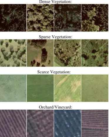
The eight classes gave rise to four new classes, more general but well distinct from each other, that are: Dense Vegetation; Sparse Vegetation; Scarce Vegetation and Orchard/Vineyard (see Fig. 2).
(a) Dense Grove
(b) Sparse
Grove (c) Glade (d) Woods
(e) Dense Bush or
Scrubs
(f) Orchard (g) Vineyard (h) Orchard/ Vineyard
Fig. 1: Classes defined by CIGeoE
(i) Dense Vegetation
(j) Sparse Vegetation
(k) Scarce Vegetation
(l) Orchard/ Vineyard Fig. 2: New classes
The first three classes are distinguished by the density of the vegetation that they represent, while the fourth stands out by represent the areas of cultivation, such as the orchards and vineyards. With these new classes is constituted a new set of training and test.
B. Training Set
Four images were extracted to represent each class, in a total of 16 train images, all with a dimension of 100x100 pixels (Fig. 3). Each image was divided into 25 ROIs with a dimension of 20x20 pixels. Subsequently it was computed the features from each ROI, which result in a training vector with a dimension of 400x86.
Dense Vegetation:
Sparse Vegetation:
Scarce Vegetation:
Orchard/Vineyard:
Fig. 3: Images used for training set
It was implemented the feature selector BFS, in order to create training sets with different numbers of features, varying from 5 to 40 in increments of 5.
C. Test Set
To establish a comparison between the two implemented classifiers, it was defined a test set. It is composed by six images, presented in Table I, all with different size and vegetation’s type and distribution. It resulted in a test set composed by 2338 ROIs.
TABLE I IMAGES OF TEST SET Image Dimension (pixels)
A 400 x 400
B 300 x 200
C 300 x 400
D 180 x 140
E 500 x 500
F 400 x 400
The comparison was done through the overall accuracy (OA), which implied a manual classification of all test image’s ROIs to use as a reference point. Then it was classified the test set with KNN and SVM. In the KNN classifier the highest OA values were obtained for 10 features, being six of them from first order. Both metrics, euclidean and mahalanobis, showed similarities.
In Fig. 4 is shown an example of classification with three classes (Dense Vegetation – green, Sparse Vegetation – blue, Scarce Vegetation – red). The first image is the original one (RGB), the second is the reference classification, the third one is the classification obtained by KNN and the last one was obtained by SVM classifier.
(a) Original image (b) Reference classification
(c) KNN classification (d) SVM classification Fig. 4: Example of classification with three classes
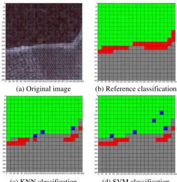
In Fig. 5 is shown another example of classification with three classes (Dense Vegetation – green, Scarce Vegetation – red, Orchard/Vineyard - grey). The first image is the original one (RGB), the second is the reference classification, the third one is the classification obtained by KNN and the last one was obtained by SVM classifier.
(a) Original image (b) Reference classification
(c) KNN classification (d) SVM classification Fig. 5: Example of classification with three classes
After several tests the best classification result, 88,3%, was achieved using mahalanobis, a � value of 5 and 10 features.
On the other hand, the SVM classifier got better results for 20 features, being 12 of them from second order. The results between the two kernels, linear and rbf, ranged from 0,9% to 10,5%. The highest OA with this classifier was 90% for 20 features, using as parameters: � = 10, � = 10=M and rbf kernel.
This was followed by the computation of OA’s mean value for each classifier, in each image, and with different number of features (Fig. 4).
Fig. 6: Average results of classifiers
The KNN classifier reaches an OA of 88% for 10 features, while the SVM classifier gets 90% for 20 features.
It was tested the influence of feature selector by comparing it with the results obtained using the 86 features of training
0% 10% 20% 30% 40% 50% 60% 70% 80% 90% 100%
5 10 15 20 25 30 35 40
O.
A
.
Number of features
set. The KNN classifier showed an OA increase of 9,25% while the SVM’s OA only increased 7,25%.
V. CONCLUSION
In order to achieve the proposed objective, it was adopted a working methodology composed by three essential steps: extraction of features, selection of features and classification of images. The CIGeoE provided aerial orthorectified photographs from Valença and Mafra, as well as eight classes they used in the discrimination of the plant cover. In these photos, regions of interest were extracted from them that enable it to represent each of these classes. These were divided into smaller regions and features of first and second order were extracted from them, allowing us to assemble a training set to teach the classifiers. Next it was implemented the BFS, that recursively eliminates those that are redundant and/or strongly correlated among themselves, allowing features’ selection that contain the most relevant information for the discrimination of the various classes. With the training set and respectively most relevant features, is applied the method GridSearchCV. This allows the achievement of input parameters of the classifiers KNN and SVM through a thorough search among all parameters assigned. This search is optimized by the use of the technique K-fold cross validation. The use of this technique leads to a decrease in the classification error. After the classifiers input parameters are estimated, each of the eight images selected are submitted and then proceeded to its classification. Like the training images, the test images are divided into ROIs with a dimension of 20 pixels per 20 pixels. Each ROI is classified as belonging to one of the classes defined.
Based on the above methodology we proceeded to obtain the results. However, the use of eight classes defined by CIGeoE does not allow to obtain satisfactory results. The classifications were close to randomness. Some classes presented a performance below 20%. It is concluded that the main cause for these poor performances was the similarity between some classes, reason why it was decided to fuse the classes to reduce this effect. The eight classes gave rise to four new classes, more general but well distinct from each other. The first three classes are distinguished by the density of the vegetation that they represent, while the fourth stands out by represent the areas of cultivation, such as the orchards and vineyards. With these new classes is constituted a new set of training and test. Next, we proceeded to features’ extraction and selection, as well as classifiers’ parameterization. Then, each image is classified with the classifiers KNN and SVM. Both present an average accuracy between 62% and 90%. In KNN’s case, we conclude that this gets the best results when 10 features are selected, being these, essentially, composed by features of first order. On the other hand, in SVM’s case, the effect observed is the opposite. The best results are obtained with the use of 20 features, where there are already present features related with texture; more specifically the features associated with uniformity and homogeneity of the ROIs. Therefore, it is concluded, that these features allow an accuracy’s
optimization for this classifier. In both classifiers, it was observed a decrease in its accuracy using even more features. Then it was tested the influence of the features selector in both classifiers and it was concluded that the use of this method leads to an average accuracy’s increase of 9,25% in the case of KNN, and 7,25% on SVM.
VI. FUTURE WORK
As a future work it would be interesting to implement segmentation before the features extraction, so the different types of vegetation would be defined by their boundaries. In each of the segmented regions, the features would be extracted and then classified. This segmentation would help to implement more specific classes, such as, the distinction between orchard and vineyard areas and may thus be possible to distinguish the eight classes initially defined.
Another solution could be the use of images with multiple resolutions, which would be made to classify the four used classes, and then each class would be divided into the original classes. As an example the class Dense Vegetation would be separated into Dense Groove and Dense Bush by the detection of the type of vegetation, in this case, tree or shrub.
ACKNOWLEDGMENTS
The author would like to thank to his family, namely his parents and sisters for all encouragement and support through the elaboration of this work. Also would like to thank to Professor José Bioucas-Dias, Professor José Silva and Major Paulo Pires for all dedications, support and guidance along this study.
REFERENCES
[1] U. Bradter, T. J. Thom, J. D. Altringham, W. E. Kunin, and T. G. Benton, "Prediction of national vegetation classification communities in the british uplands using environmental data at multiple spatial scales, aerial images and the classifier random forest.(report)," Journal of Applied Ecology, vol. 48, no. 4, p. 1057, 2011.
[2] D. Lewis, S. Phinn, and L. Arroyo, "Cost-effectiveness of seven approaches to map vegetation communities — a case study from northern australia’s tropical savannas," Remote Sensing, vol. 5, no. 1, pp. 377-414, 2013.
[3] A. Laliberte, D. Browning, J. Herrick, and P. Gronemeyer, "Hierarchical object-based classification of ultra-high-resolution digital mapping camera (dmc) imagery for rangeland mapping and assessment," Journal of Spatial Science, vol. 55, no. 1, pp. 101-115, 2010.
pca with application to object-based vegetation species classification," IEEE 17th International Conference on Image Processing, pp. 2701-2704, 2010.
[5] D. S. Chapman, A. Bonn, W. E. Kunin, and S. J. Cornell, "Random forest characterization of upland vegetation and management burning from aerial imagery," Journal of Biogeography, vol. 37, no. 1, pp. 37-46, 2010.
[6] Minho Kim, Timothy A. Warner, Marguerite Madden, Douglas S. Atkinson, "Multi-scale GEOBIA with very high spatial resolution digital aerial imagery: scale, texture and image objects," International Journal of Remote Sensing, vol. 32, no. 10, pp. 2825-2850, Maio 2011.
[7] M. Arebey, M. Hannan, R. Begum, and H. Basri, "Solid waste bin level detection using gray level co-occurrence matrix feature extraction approach," Journal of Environmental Management, vol. 104, pp. 9-18, 2012. [Online].
http://www.sciencedirect.com/science/article/pii/ S0301479712001545
[8] Guyon, I., & Elisseeff, A., "An introduction to variable and feature selection," The Journal of Machine Learning Research, pp. 1157-1182, 2003.
[9] I. Guyon and A.Elisseen, An Introduction to variable and feature selection.: J. Mach. Learn. Res, 2003, vol. 3. [10] C. Romero, M. Valdez, and A. Alanis, "A comparative study of machine learning techniques in blog comments spam filtering," The 2010 International Joint Conference on Neural Networks (IJCNN), pp. 1-7, 2010.
[11] I. Saini, D. Singh, and A. Khosla, "
[12] J. Ramirez-Cortes, P. Gomez-Gil, V. Alarcon-Aquino, J. Gonzalez-Bernal, and A. Garcia-Pedrero, "Neural networks and SVM-based classification of leukocytes using the morphological pattern spectrum," Soft Computing for Recognition based on Biometrics, Studies in Computational Intelligence, 2010.
[13] Christopher M. Bishop, Pattern Recognition and Machine Learning.: Springer, 2006.
[14] Y. Liu, J. Lian, M. R. Bartolacci and Q.A. Zeng, "Density-based penalty parameter optimization on c-svm," The Scientific World Journal, pp. 814-815, 2014.
[15] Nathalie Long, Arnaud Bellec, Erwan Bocher, Gwendall Petit, "Influence of the methodology (pixel-based vs object-based) to extract urban vegetation from VHR images in different urban zones," 5th Geobia Conference, 2014.
[16] Soe W. Myint, Patricia Gober, Anthony Brazel, Susanne Grossman-Clarke, Qihao Weng, "Per-pixel vs. object-based classification of urban land cover extraction using high spatial resolution imagery," Remote Sensing of Environment, vol. 115, no. 5, pp. 1145-1161, May 2011.
Joel Augusto Joanaz D’Assunção Dias