N
EIGHBORHOOD
I
NFORMATION
E
XCHANGE
AND
V
OTER
P
ARTICIPATION
:
A
N
E
XPERIMENTAL
S
TUDY
*by
Jens Großer
i,iiArthur Schram
iABSTRACT
We study the effect of social embeddedness on voter turnout by investigating the role of information about other voters’ decisions. We do so in a participation game, where some voters (‘receivers’) are told about some other voters’ (‘senders’) turnout decision at a first stage of the game. Cases are distinguished where the voters support the same or different candidates or where they are uncertain about each other’s preferences. Our experimental results show that such information matters. Participation is much higher when information is exchanged than when it is not. Senders strategically try to use their first mover position and some receivers respond to this.
this version: May 2004
i
Center for Research in Experimental Economics and political Decision making, University of Amsterdam; Roeterstraat 11, 1018 WB Amsterdam, the Netherlands.
ii
Department of Economics, University of Cologne; Albertus-Magnus-Platz, 50923 Cologne, Germany.
email: [email protected]; [email protected]
*
1. INTRODUCTION
The ‘voter paradox’ of why substantial portions of large electorates turn out to vote has puzzled economists since Downs (1957). In the Downsian framework, the probability of being pivotal in large-scale elections is negligible and, therefore, expected revenues from casting a vote fall short of the costs. Many theoretical and empirical papers have been published trying to explain the paradox, but not until the nineteen-eighties did rational choice models start to appear that show that turning out to vote might be rational in an instrumental sense (see Ledyard 1984, or Schram 1991, and the references given there).
Palfrey and Rosenthal (1983) model the turnout decision as a participation game and study it game-theoretically. In this game, there are two or more teams. Everyone has to make a private decision on whether or not to ‘participate’ in an action, where participa-tion is costly. Participaparticipa-tion is beneficial to every member in one’s own team and harmful to members of other teams. The team with the higher number of ‘participants’ gets the (higher) reward. Palfrey and Rosenthal show that in some cases Nash equilibria with sizeable levels of participation exist. However, when the game allows for substantial uncertainty about voters’ preferences and costs, equilibria with high participation generally disappear (Palfrey and Rosenthal, 1985).1
The participation game simultaneously combines two kinds of conflict: a between-group conflict for the higher reward, and a within-between-group conflict, where each between-group member has an incentive to free ride on costly participation by other members of the own group. For any given number of players in the other group choosing to participate, the resulting game in the own group boils down to a voluntary contribution mechanism with a step-level public good (e.g., Offerman et al., 1996).
The experimental literature on participation games is still quite limited. Bornstein (1992) was the first to use experiments to study participation in small groups. Schram and Sonnemans (1996a,b) vary group size and compare elections of proportional representation to winner-takes-all elections. Hsu and Sung (2002) investigate participation for equally sized groups in electorates with up to 70 voters. Cason and Mui
1
(2003) use the participation game to model reforms and study the impact of payoff uncertainty and varying costs. Finally, Großer etal. (2004) study the effect of preference uncertainty and differences between allied and floating voters. In all of these studies, relatively high rates of participation are found, albeit that lower turnout is observed than in most general elections around the world. Moreover, a typical result in these studies is that the standard Nash equilibria find little support. However, Goeree and Holt (forthcoming) show that a logit equilibrium can account for the Schram and Sonnemans data and Cason and Mui show the same for their own data.
In this paper, we focus on a voter’s social environment. An important element of this environment is the information exchanged within it. Here, we explore this exchange of information in an attempt to take the study of voter turnout one step further, whilst maintaining the participation game framework. We do so by giving voters information about the turnout decision of some other voter in their surrounding. This is inspired by the idea that it is quite natural for interaction to take place before and during elections amongst individuals in small social environments or neighborhoods (e.g., a family or working place). Of course, this interaction can be very complex and take on a variety of forms. We are interested in the exchange of information between voters about the candidates they support, and especially about their decision on whether or not to vote. To the best of our knowledge, there has been no thorough analysis to date of how such ‘neighborhood information exchange (NIE)’ may influence voter participation. We extend the participation game to include NIE and study this game both theoretically and experimentally.
In our model, we focus on neighborhoods that consist of two voters only.2 Information exchange between these voters has two dimensions. First, neighbors know whether they support the same or opposing candidates (or that they are uncertain about each other’s preferences). Second, one of them can observe whether her neighbor-voter has cast a vote or not. For this, we distinguish between voters who send information and
2
those who receive it.3 This allows us to explicitly study the influence on participation in both roles. The (endogenous) content of information in our setting is the sender’s decision whether or not to vote, which is observed by her receiver-neighbor.
In our NIE participation game decisions are made in two stages. There are two (equally sized) groups of players, or voters, and within each group an equal number of senders and receivers of information is distinguished. At stage 1, each sender decides whether to participate or abstain. Each sender knows that (only) her receiver-neighbor will observe this decision. If the sender participates, she does not take part in stage 2. If she abstains, she again decides on participating or abstaining at stage 2, but this time she knows that this decision will not be observed. At stage 2, receivers decide whether or not to participate, knowing their sender-neighbor’s stage 1 decision. Note that neither senders nor receivers observe others’ stage 2 decisions. The outcome of the game is determined by counting all stage 1 and 2 participation in the two groups, with the higher reward going to the members of the group with the highest participation (with a coin toss deciding in case of a tie).
Though neighborhood information exchange has not been studied in a participation game before, various studies of voting contain elements that are relevant for our set-up. Of special interest are results that relate to the influence on voter participation of (i) social embeddedness and communication and (ii) procedures that combine simultaneous and sequential voting.
We start with a brief discussion of some of the literature concerning the first of these two areas. Putnam et al. (1993) argue that there is an important link between a society’s social capital and the level of voter turnout at its elections. Carlson (1999) provides empirical support. One interesting aspect of social embeddedness is whether interaction takes place between allies or adversaries. Schram and van Winden (1991) argue that so-cial pressure and examples set by group leaders play an important role in a voter’s
3
sion. Moreover, there is evidence from empirical and simulation studies that segregation increases voter participation (e.g., Butler and Stokes 1974; Ragin 1986; Takács 2001, 2002). Communication is an important aspect of social embeddedness. Schram and Sonnemans (1996b) show that both group identity and within-group communication increase turnout in experimental participation games. Goren and Bornstein (2000) find the same; in addition, they also show that groups use the opportunity of communication to coordinate on a reciprocal strategy towards the other group. All in all, interaction and within-group communication appears to have a positive effect on voter participation.
With respect to the second area of interest, first note that many elections involve elements of both simultaneous and sequential voting. In sequential voting, voters make their decisions knowing earlier voters’ (turnout) decisions in the same election. In simultaneous voting, no voter receives information about any others’ prior decision.4 A prime example where elements of both are mixed is in the US presidential primaries (e.g., Bartels, 1988; Morton and Williams, 1999, 2000). Morton and Williams (1999) argue that there, voting has been moving from sequential to simultaneous since states began (in the 1980s and 1990s) to move their primaries closer together at the beginning of the season. This shift yields more uninformed decisions, since voters have fewer oppor-tunities to learn about the candidates from previous elections. Learning from early voters’ decisions (e.g., about candidates, voter preferences, or ‘states of the world’) is at the core of most studies in this field. These investigate the ability of elections to aggregate information in models of incomplete information.
We know of a few prominent studies that (like ours) combine sequential with simultaneous voting. Morton and Williams (1999) explore US presidential primaries theoretically and experimentally by comparing pure simultaneous versus pure sequential voting over three candidates, where voting is mandatory. In the sequential setting, half of the voters simultaneously decide first. The outcome is made public, from which voters can learn about candidates’ types. Then, the other half votes. In the experiment, Morton
4
and Williams find, i.a., that early voters generally vote informatively and that later voters use early outcomes to make decisions that better reflect their preferences.
Lohmann (1994a) models pre-election costly political action, through which voters can signal their private information about policy alternatives to other voters (e.g., through petitions and demonstrations). Lohmann (1994b) presents empirical evidence for this model. Observing the number of political actions, voters update their own information and cast a mandatory vote at the election stage. Lohmann finds, i.a., that political action prior to elections may be counterproductive, i.e. full-information voting outcomes become less likely with such action.
Dekel and Piccione (2000) present a voting game with incomplete information about others’ preferences over two policy alternatives. Their main result is that (informative) symmetric equilibria of the game with simultaneous voting are equilibria for any
sequential voting structure as well. The model includes endogenous timing of decisions and allows for both common and private values to the voters. Contrary to the previous two studies, this model includes the option to abstain in the elections. However, Battaglini (2004) shows that the main result no longer applies when voting costs are introduced.
The models discussed focus on the ability of sequential procedures to increase electoral efficiency by spreading private information (about policies or voter preferences) from early decisions to late voters. This is how they differ from our study, in which incomplete information is not essential. Rather, we are interested in the exchange of information about participation decisions within neighborhoods, where preferences are known (we only use incomplete information in one case, where voters do not know which candidate their neighbor supports).
reports that this news decreased the turnout of voters who had not yet participated. Both, Democrats and Republicans, were negatively affected, though the Reagan supporters more strongly so. Jackson (1983, p.632) suggests “the early reporting of projections may only alter turnout in elections in which the projections differ from prior expectations. Elections in which people anticipate a close race, but in which the early returns and projections indicate the opposite, are the situations we expect to see a drop in turnout directly related to the media’s coverage”.
We can compare Jackson’s approach to ours. First, in his study ‘late’ voters receive information about aggregate turnout of a subgroup of voters, i.e., East coast citizens. In the NIE participation game, on the other hand, turnout information is on a much smaller scale, about a single voter. Secondly, as a consequence, Jackson’s study contains mixed information about participation of allies and adversaries, whereas our aim is to decompose the effects of these distinct kinds of information. Note that our laboratory experiment allow us to do so. Thirdly, the NIE participation game maintains an important feature of Jackson’s study, namely that East coast citizens who had not yet voted, still had the opportunity to participate after the projection has been made public. This makes their situation comparable to senders in the NIE participation game. In this respect, our distinction between senders and receivers complements the empirical results of Jackson. Finally, the outcome in the 1980 US presidential election was expected to be close. In our study, we impose closeness by using equal group sizes (cf. Großer etal. 2004).
twofold: first, looking at previous comparisons of partners versus strangers in experimental participation games (Schram and Sonnemans, 1996a; Großer et al. 2004), we would expect higher participation by partners. Second, we expect that the relative importance of NIE is more important in strangers. With fixed groups, aggregate behavior is supposedly more predictable, which may decrease the value of observing the neighbor’s decision as compared to the case when group composition varies. Hence, we would expect that receivers respond more to neighbors’ first stage decisions in strangers than in partners, and senders would anticipate this.
The remainder of this paper is organized as follows. Section 2 defines the NIE participation game and discusses its equilibria. In section 3, we describe the experimental design and in section 4 our experimental results are presented and analyzed. We conclude in section 5.
2. THE NIE-PARTICIPATION GAME
2.1THE GAME
The NIE participation game has two stages. We assume an even and equal number of risk neutral players (voters) N =NA =NB in each of two groups i= A,B.5 Half of the voters in each group is of the type S(ender), denoted by ji,S, i= A,B, and the other half of the type R(eceiver), ji,R, i= A,B. Hence, each group consists of Ni,S = N 2 senders and
2
, N
NiR = receivers. Each voter knows her own type.
DEFINITION 1 (neighborhood ϑ)
A neighborhood ϑ is a matched pair of exactly one sender and one receiver.
Denote the neighbor of ji,S by n(ji,S) and the neighbor of ji,R by n(ji,R). Each voter is member of exactly one neighborhood. Hence, there are N neighborhoods in the electorate.
5
DEFINITION 2 (matching protocol Θ)
We distinguish three matching protocols Θ. The sender and receiver in a neighborhood are either from
1. the same group, ϑ∈Θown⇒
[
ji,S ∈i⇔n(ji,S)∈i] [
∧ ji,R ∈i⇔n(ji,R)∈i]
; 2. different groups, ϑ∈Θother⇒[
ji,S ∈i⇔n(ji,S)∉i] [
∧ ji,R∈i⇔n(ji,R)∉i]
;3. an uncertain group, ϑ∈Θuncertain, where Θown occurs with probability 1
) (
0< prob Θown < and Θother with prob(Θother) =1− prob(Θown).
All N neighborhoods ϑ have the same matching protocol, which is common knowledge. The interpretation of definition 2 is that voters either know with certainty which candidate their neighbor supports (Θown and Θother), or have only probabilistic knowledge (Θuncertain) about her preferences. In the following, if the matching protocol
m
Θ , m=own,other,uncertain, is not explicitly mentioned, a general case valid for all matching protocols will be under consideration.
The following structure and rules of the game are common knowledge to all players. At stage 1 all NA,S +NB,S senders simultaneously decide whether to vote 1
1 ,S = i
j
v , or
abstain, 1 0
,S = i
j
v , i= A,B, where superscript ‘1’ refers to stage 1. Each receiver ji,R
observes (only) the sender n(ji,R)’s decision and no other voter observes this decision. Senders who turn out to vote at stage 1 have no further decision to make, whereas senders who abstain at stage 1 have to decide again on voting at stage 2.
At stage 2, all NA,R +NB,R receivers and all senders who abstained at stage 1 simultaneously decide whether to vote, 1; 1
, ,
2 = =
R i S
i j
j v
v , or abstain, 2 0;
,S =
i
j
v 0
,R =
i
j
v ,
B A
i= , , where superscript ‘2’ indicates stage 2 for senders. After all decisions have been made, voters are told the aggregate outcome of the election (the total number of votes cast in each group). No additional information about any other voter’s turnout decision is given.
≡∑
(
+)
+∑R
i iR
S
i iS iS j j
j j j
i v v v
V
, ,
, , ,
2 1
, (1)
where 1 2
, ,S iS i j
j v
v + ∈ {0,1}, because senders can cast only one vote. For later use, we define the aggregate turnout of other voters in the same group as sender ji,S, or receiver
R i
j, , i= A,B, by
(
1 2)
, , , S i S i S i j j i j
i V v v
V− ≡ − + ; (2a)
R i R i j i j
i V v
V
,
, ≡ −
−
. (2b)
Revenues (the gross payoff to each member of the winning group) are denoted by w and assumed to be equal for senders and receivers in a group ( =
i j w = S i j w
, wji,R, i= A,B):
(
)
> = < = − − − − , 1 0, 12
i i i i i i i i j V V if V V if V V if V V w i (3) B A
i= , , where −i refers to the opposing group. Furthermore, we assume identical participation costs to all voters, independent of type and stage, within the range c∈(0,1),
S i j,
∀ , ∀ji,R, i= A,B. The common knowledge payoffs (denoted by π) for senders ji,S,
and receivers ji,R, i= A,B, are then given by
(
V V)
(
v v)
c w S i S i i Si j i i j j
j , 2 1 , , , = − − +
π ; (4a)
(
V V)
v c wR i i
R
i j i i j
j, = , − − ,
π . (4b)
In what follows, it will be useful to define the number of senders in group i, who vote at stage 1 by
≡
∑
S i iS
j j
i v
S
, ,
1
. (5)
In case of matching protocol Θown, Si is also the number of receivers in i who observe a sender voting at stage 1. For matching protocol Θother, this number is given by S−i.
2.2NASH EQUILIBRIA
derived.6 More details are available from the authors. Because notations can become cumbersome, we apply Kuhn’s theorem (1953) by analyzing ‘behavioral’ rather than mixed strategies. This will allow us to consider strategies at each stage separately as opposed to strategies for the complete game.
First, we consider the four situations a voter in group i= A,B, facing matching protocol Θm, m=own,other,uncertain, might be in:
1) a sender deciding on 1 ( )
, m
jiS
v Θ at stage 1;
2) a sender having abstained at stage 1, 1 ( ) 0
,S Θm =
i j
v , and deciding on
) (
2
, m
jiS
v Θ at stage 2;
3a) a receiver deciding on ( 1( ) 0, )
,
, n j m
jiR v iR
v = Θ at stage 2 after observing her neighbor abstaining at stage 1;
3b) a receiver deciding on ( 1( ) 1, )
,
, n j m
jiR v iR
v = Θ at stage 2 after observing her neighbor voting at stage 1.
Behavioral strategies for each of these situations are, respectively, the probabilities:
1) ( )
, m
jiS
s Θ that 1 ( ) 1
,S Θm =
i j
v ; (6a)
2) ( )
, m
jiS
a Θ that 2 ( ) 1
,S Θm =
i j
v ; (6b)
3a) ( )
, m
jiR
a Θ that ( 1 ) 0, ) 1
, (
,R n jiR = Θm =
i
j v
v ; (6c)
3b) ( )
, m
jiR
t Θ that ( 1 1, ) 1
) , (
,R n jiR = Θm =
i
j v
v . (6d)
A voter will vote with probability 1 if the expected benefits minus the costs c are higher than the expected benefits from abstention. She will mix when the two are equal. This yields the following four turnout conditions (7)-(10) for the situations distinguished.
CONDITION 1(senders, stage 1):
Sender ji,S will vote with probability 1 at stage 1 ( ( ) 1
,S Θm =
i j
s ) iff
[
]
[
1 ( ) 1]
[
[
1 ( ) 0]
]
,, , 2 1 , , 2
1 strat j j Θm = > strat strat j j Θm =
strat Exp iS viS Exp Exp iS v iS
Exp π π
6
where expectation operators are due to (i) strategic uncertainty about others’ decisions at stage 1 (strat1); and (ii) strategic uncertainty about others’ decisions at stage 2 (strat2), given the number of votes at stage 1 in each group. Elaborating gives:
[ ]
i[ ]
i N S N S S prob S prob i i − = =∑
∑
− 2 0 2 1 ×(
)
Θ > + − − − i i m i ji V S S
V prob iS
, , 1
,
prob Vi jiS V i
(
m Si S i)
−c Θ = +
+ − 1 − , , −
2
1 ,
[ ]
i[ ]
i N S N S S prob S prob i i − − = − =∑
∑
−> 2 0 0 1 2 0 ×
(
)
Θ > − − i i m i ji V S S
V
prob i,S , ,
prob V V
(
S S)
v cS i S i j i i m i j i 2 , , , , 2 1 − Θ =
+ − − − , (7)
B A
i= , , for m=own,other. The prob[S] terms in (7) refer to the stage 1 votes by senders in the two groups.7 The first term after the multiplication operator on the left (right) hand side of the inequality describes the probability that this sender’s group i will win the election if she votes (abstains) and the second term describes the probability that i
will tie the election if ji,S votes (abstains) at stage 1. Note that, in case of abstention at stage 1, the sender still has to account for possible costs at stage 2.
CONDITION 2 (senders, stage 2): Similarly, sender ji,S will vote with probability 1 at stage 2 iff the expected payoff of turnout is higher than that of abstention:
[ ]
i[ ]
i N S N S S prob S prob i i − − = − =∑
∑
− 0 2 0 1 2 0(
)
= Θ > +× −j −i m j i −i
i V v S S
V prob S i S i , , 0 , 1 1 , ,
(
v S S)
cV V
prob i j i m j i i
S i S i − = Θ = +
+ − 1 − , 0, , −
2 1 1 , , 7
[ ]
i[ ]
i N S N S S prob S prob i i − − = − =∑
∑
−> 2 0
0 1 2 0
Θ =
>
× −j −i m j i −i
i V v S S
V prob S i S i , , 0 , 1 , ,
Θ =
=
+ −j −i m j i −i
i V v S S
V prob S i S i , , 0 , 2 1 1 , , , B A
i= , , for m=own,other. Rearranging gives
[ ]
i[ ]
i N S N S S prob S prob i i − − = − =∑
∑
− 0 2 0 1 2 0(
)
= Θ = +× −j −i m j i −i
i V v S S
V prob S i S i , , 0 , 1 1 , ,
(
)
= Θ =+ −j −i m j i −i
i V v S S
V prob S i S i , , 0 , 1 ,
, >2c (8)
CONDITION 3a (receivers at stage 2 after observing abstention): Given 1( ) 0
,R =
i
j n
v , the
expected payoff from voting exceeds that from abstention when:
[ ]
i[ ]
i y N S x N S S prob S prob i i − − = − = ∑ ∑ − 2 0 2 0(
)
= Θ > +× −j −i m n j i −i
i V v S S
V prob R i R i , , 0 ,
1 1( )
,
,
(
v S S)
cV V
prob i j i m n j i i
R i R i − = Θ = +
+ − 1 − , 0, , −
2
1 1
) ( , ,
[ ]
i[ ]
i y N S x N S S prob S prob i i − − = − = ∑ ∑ − > 2 0 2 0(
)
= Θ >× −j −i m n j i −i
i V v S S
V prob R i R i , , 0 , 1( )
, ,
(
)
= Θ =+ −j −i m n j i −i
i V v S S
V prob R i R i , , 0 , 2 1 1 ) ( , , , B A
i= , , where x=1; y=0 for m=own, and x=0; y=1 for m=other.8 Rearranging gives
8
In own, Si∈{0,...,N/2−1} because i observed a stage 1 abstention in the own group. Similarly
} 1 2 / ,..., 0 { − ∈ − N
[ ]
i[ ]
i y N S x N S S prob S prob i i − − = − = ∑ ∑ − 2 0 2 0(
)
= Θ = +× −j −i m n j i −i
i V v S S
V prob R i R i , , 0 ,
1 1( )
, ,
(
)
= Θ =+ −j −i m n j i −i
i V v S S
V prob R i R i , , 0 , 1( )
,
, c
2
> (9)
CONDITION 3b (stage 2): (receivers at stage 2 after observing a vote): Given 1( ) 1
,R = i
j n
v ,
the expected payoff from voting exceeds that from abstention when:
[ ]
i[ ]
i N y S N x S S prob S prob i i − = = ∑ ∑ − 2 2(
)
= Θ > +× −j −i m n j i −i
i V v S S
V prob R i R i , , 1 ,
1 1( )
,
,
prob Vi j V i
(
m vn j Si S i)
c R i R i − = Θ = ++ − 1 − , 1, , −
2
1 1
) ( , ,
[ ]
i[ ]
i N y S N x S S prob S prob i i − = = ∑ ∑ −> 2 2
(
)
= Θ >
× −j −i m n j i −i
i V v S S
V prob R i R i , , 1 , 1( )
, ,
(
)
= Θ =+ −j −i m n j i −i
i V v S S
V prob R i R i , , 1 , 2 1 1 ) ( , , , B A
i= , , where x=1; y=0 for m=own, and x=0; y=1 for m=other.9 Rearranging gives
[ ]
i[ ]
i N y S N x S S prob S prob i i − = = ∑ ∑ − 2 2(
)
= Θ = +× −jR −i m n j i −i
i V v S S
V prob
R
i 1, ,
,
1 1( )
,
(
)
= Θ =+ −j −i m n j i −i
i V v S S
V prob R i R i , , 1 , 1( )
, ,
c
2
> (10)
The conditions for Θuncertain are a probability mix of the respective conditions with probabilities prob(Θown) and prob(Θother). This gives a game of incomplete information.
9
Next, we define the equilibria considered for this NIE participation game.
DEFINITION 3 (Quasi-symmetric equilibrium)
An equilibrium in behavioral strategies in the NIE participation game is quasi-symmetric if it holds that:
] 1 , 0 [ ,
, =s ≡s ∈
s
S k S
i h
j , ∀ji,S, hk,S, i,k = A,B,
] 1 , 0 [ ,
, = h ≡ S ∈
j a a
a
S k S
i , ∀ji,S, hk,S, i,k = A,B,
] 1 , 0 [ ,
, = h ≡ R ∈
j a a
a
R k R
i , ∀ji,R, hk,R, i,k = A,B, and
] 1 , 0 [ ,
, =t ≡t∈
t
R k R
i h
j , ∀ji,R, hk,R, i,k = A,B. (11)
In words, all voters in any particular decision situation play the same behavioral strategy, independent of the group they are in. This reduces our equilibrium analysis to four strategies. The equilibrium is denoted by ‘quasi-symmetric’ because strategies are not limited to be symmetric across players in different positions.
PROPOSITION (Quasi-symmetric Nash equilibria in pure strategies):
(i) If c>12, the only Nash equilibrium is where nobody votes: 1 ( ) 0
, Θm =
jiS
v ,
0 ) (
2
, Θm =
jiS
v , ( 1( ) 0, ) 0
,
, n j = Θm =
jiR v iR
v , ( 1( ) 1, ) 0
,
, n j = Θm =
jiR v iR
v , ∀ji,S, ∀ji,R,
B A
i= , , m=own,other,uncertain.
(ii) If c<1 2, the only Nash equilibria in pure strategies are where everybody votes:
Θ = ∧ Θ =
0 ) ( 1 )
( 2,
1
,S m jiS m
i
j v
v ∨
Θ = ∧
0 ) (
1
,S m
i j
v v2ji,S(Θm)=1,
1 ) , 0 ( 1( )
,
, n j = Θm =
j
R i R
i v
v , and ( 1( ) 1, ) 1
,
, n j = Θm =
jiR v iR
v , ∀ji,S, ∀ji,R, i= A,B,
uncertain other
own
m= , , .
To find quasi-symmetric equilibria in behavioral strategies (separately for the distinct information conditions Θm), first the decision at stage 2 is elaborated (backwards induction), using conditions (8), (9) and (10) stated as equalities. The probabilities in these equations are tedious but straightforward combinations of binomials using the probabilities defined in definition 3. This gives three equations for the four probabilities
, , ,aS aR
s and t. Senders at stage 1 anticipate the best responses implicit in these equations and will mix with a probability s that equates the expected value of voting and abstaining (eq. 7), once again involving a combination of binomials. This gives a fourth equation for the four probabilities. In the following section, we will present the equilibria derived for the parameters in our experiments.
3. EXPERIMENTAL DESIGN
The computerized10 experiment was run between April and June 2001 at the laboratory of the Center for Research in Experimental Economics and political Decision making (CREED) of the University of Amsterdam. Subjects were recruited from the university’s undergraduate population. 168 subjects participated in 10 sessions. Each session lasted about 2 hours (cf. appendix B for the read-aloud instructions). Earnings in the experiment are measured in tokens. At the end of a session token earnings were transferred to cash at a rate of 4 tokens to one Dutch Guilder (≈ € 0.45). On average, subjects earned 48.66 Guilders.
Each electorate consists of 12 voters: two groups of 6 subjects each. In 4 sessions, two electorates participated simultaneously, and 6 sessions were held with one electorate each. In sessions with more than one electorate, there is no interaction of any kind between subjects in different electorates. This is known to all subjects. Hence, each of the 14 electorates in our sessions provides us with one independent observation. Each subject is either sender or receiver throughout the experiment and knows her role from the beginning of the session. There are always 3 senders and 3 receivers in each group.
10
Our first treatment is related to the matching protocol of subjects within an electorate, where we distinguish ‘partners’ and ‘strangers’ (cf. Andreoni, 1988). In ‘partners’, subjects in an electorate are randomly allocated to groups at the beginning of the first round, and groups remain constant thereafter. In ‘strangers’, groups are randomly rematched at the beginning of each round. Note that strangers do remain in the same electorate across rounds; they are only reallocated to the two groups the electorate consists of. A natural interpretation of partners versus strangers in this context is that partners constitute an electorate of voters who remain loyal to their party across elections. Strangers can be seen as ‘floating voters’ who may switch from one party to another between elections (cf. Großer etal. 2004). Of course, partners and strangers are varied in a between-subject design.
Our second treatment is varied in a within subject design. This deals with the information about the neighbor’s vote. If voters are ‘informed’, we distinguish rounds in which neighbors are from the same (‘own’) and different (‘other’) groups, and rounds in which ‘own’ and ‘other’ each occur with probability of 0.5 (‘uncertain’). As a control, we organized four ‘uninformed’ electorates in which no information about others’ votes was provided. In these sessions we keep the decision structure as close as possible to ‘informed’ by maintaining the two decision making stages described above as well as the labels ‘sender’ and ‘receiver’. In the analysis below, we will refer to subjects in these sessions as neighbors, senders, and receivers even though no information was exchanged between them.
Each session lasts 99 decision rounds. 33 rounds use the information condition ‘own’, 33 use ‘other’, and 33 use ‘uncertain’.11 This is varied in a random, but predetermined manner (see the table in Appendix A-1 for the complete sequence). In each round, each subject in the winning group receives a revenue of 4 tokens and each subject in the losing
11
group of 1 token. Participation costs are 1 token, independent of a subject’s role. Hence, negative payoffs are avoided. Table 1 summarizes treatments and parameters.
TABLE 1:SUMMARY OF TREATMENTS AND PARAMETERS
Treatment
# Rounds (per info-condition)
Revenue win (lose)
Partici-pation costs
Size of electorate
(groups)
# Senders (receivers)
per group
Independent observations (sessions)
IP 99 (33) 4 (1) 1 12 (6) 3 (3) 5 (3)
IS 99 (33) 4 (1) 1 12 (6) 3 (3) 5 (3)
US 99 (33) 4 (1) 1 12 (6) 3 (3) 4 (4)
Note: ‘I’ = ‘informed’, ‘U‘ = ‘uninformed’, ‘P’ = ‘partners’, and ‘S’ = ‘strangers’.
For these parameters, we can derive the quasi-symmetric Nash equilibria as described in section 2 for the stage game. Normalizing revenue to lie between 0 and 1, we have
3 / 1
=
c . Following the proposition, we conclude that everyone casting a vote (with senders casting it either at stage 1 or at stage 2) is a Nash equilibrium in pure strategies12. For m=own and m=other, the quasi-symmetric equilibria in behavioral strategies13 for the stage game are given in table 2. For m=uncertain, no such equilibria exist. Using backwards induction, these equilibria hold for each round, in partners and strangers.14
TABLE 2:QUASI-SYMMETRIC NASH EQUILIBRIA IN BEHAVIORAL STRATEGIES
Treatment s aS
Expected turnout senders
t aR
Expected turnout receivers
Expected turnout
Informed
own .791 1 1 .119 1 .303 .652
.689 1 1 .560 1 .697 .848
other .406 .839 .904 .764 1 .904 .904
uncertain −
Uninformed .107 or .893*
Strategies: s= senders at stage 1; aS= senders at stage 2; t= receivers after observing participation, R
a = receivers after observing abstention.
*Any combination of probabilities s and aS that yields s+(1−s)aS= .107 or .893 is an equilibrium.
12
This is easy to confirm for the parameters chosen. A unilateral deviation from 100% turnout saves 1 token but decreases the expected revenue from 2.5 to 1.
13
In some cases, some voters do not mix in equilibrium.
14
Note that there are two equilibria for m=own.15 Moreover, equilibria are the same for partners and strangers. Table 2 shows that expected overall participation is higher for
other (.904) than for own (.652 and .848).16 Uninformed provides the lowest (.107) and a very high (.893) expected turnout, which makes it difficult to formulate comparative statics predictions vis-à-vis the informed cases. For informed, a comparison of equilibria does provide such predictions, however. In the equilibria for own, senders participate at substantially higher rates than receivers in both equilibria (1 vs. .303 and 1 vs. .697), whereas they participate at equal rates (.904) in the equilibrium for other. Also, note that in all cases, in equilibrium, senders participate at higher rates at stage 2 than at stage 1. Note that stage 2 participation rates are defined as the fraction of senders that abstained at stage 1. As a fraction of all senders, participation is higher at stage 1 than at stage 2 in
own (.791 vs. .209 and .689 vs. .311), and higher at stage 2 in other (.406 vs. .498). Finally, equilibrium participation by receivers is higher after observing abstention than after observing a sender casting a vote. The difference is largest for own.
Summarizing, we can use these Nash equilibria to formulate five hypotheses with respect to the comparative statics between own and other in our design:
H1: Turnout is higher when neighbors are adversaries than when they are allies. H2: When they are allies, senders participate at a higher rate than receivers. H3: Senders participate at higher rates at stage 2 than at stage 1.
H4: Receivers participate more after observing abstention than after observing a vote.
H5: After observing a vote, receivers are more likely to participate if the neighbor is an adversary than in case of an ally.
We will return to these comparative statics, when presenting our results.
15
The two equilibrium strategies for receivers are also a ‘low’ (.303) and ‘high’ (.697) equilibrium in the standard participation game (Palfrey and Rosenthal, 1983) with the same voting costs but two groups of equal size 3. This is intuitive, since all 6 senders vote with probability 1 in own, hence creating a tie and the remaining receivers play a participation game of three against three.
16
4. EXPERIMENTAL RESULTS
This section presents and analyzes our experimental results. We start with overall participation for all treatments, followed by an investigation of participation rates in the three information conditions. Then, our focus will be on behavior of senders at stages 1 and 2 and receivers. For the latter, we distinguish between cases where they observed turnout or abstention by their sender-neighbors. After discussing electoral efficiency and realized earning distributions, we will try to put the pieces of the puzzle together and get a grasp of what the effect of NIE is. For our analysis we use nonparametric statistics as described in Siegel and Castellan, Jr. (1988). As mentioned above, our data provide independent observations at the electorate level. Therefore, all of our tests will be conducted at the electorate level.
4.1AGGREGATE PARTICIPATION RATES
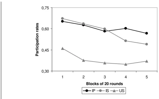
Figure 1 gives aggregate participation rates averaged over blocks of 20 rounds each (19 rounds in the last block).
FIGURE 1:AGGREGATE PARTICIPATION RATES.
0,30 0,45 0,60 0,75
1 2 3 4 5
Blocks of 20 rounds
P
a
rt
ic
ipa
tion r
a
te
s
IP IS US
RESULT 1: Neighborhood information exchange increases turnout.
rounds 1-20 and ends at 49% in rounds 81-99. At the same time, average participation in US varies between 46% and 37%. The null hypothesis of no difference is clearly rejected at the electorate level: there is not one observation in US that exceeds those in IS (one-tailed Wilcoxon-Mann-Whitney test, 1% significance level).
RESULT 2: The stability of group composition does not affect turnout.
In our design, the stability of group composition is varied by way of our partners versus strangers treatments. IP and IS start at participation rates of 65% and 67%, respectively, decreasing to 57% and 49%. A Wilcoxon-Mann-Whitney test cannot reject the null hypothesis of no difference (10% significance level, two-tailed test).17
In US, observed aggregate participation rates are at similar levels to those observed in previous experimental studies on participation games without information exchange. For example, Schram and Sonnemans (1996a) report average turnout rates of 31% (42%) for the winner-takes-all case with two groups of 6 players in strangers (partners). For strangers, this is somewhat lower than what we observe in US (38%). Aggregate participation rates in the two informed treatments are much higher than previously observed for both partners and strangers.
We can also compare our results to the Nash equilibria shown in Table 2. It appears that turnout is lower than predicted by the quasi-symmetric equilibria for informed voters and between the two predictions for the uninformed.18 We will consider the relationship between observed behavior and equilibrium predictions in more detail, below.
4.2PARTICIPATION RATES PER INFORMATION CONDITION
Figure 2 shows participation rates disaggregated for the information conditions own,
other, and uncertain for IP and IS, respectively.19
17
Figure 1 suggests that a difference may occur in the last two blocks. The test does not reject the null hypothesis of no differences for these blocks either, however.
18
For this aggregate case, we cannot conclude much about the comparative statics implied by the equilibria. For one of the two equilibria for US, the observed higher participation by the informed is in line with the equilibrium comparative statics, for the other it is not.
19
FIGURE 2A:PARTICIPATION RATES PER INFORMATION CONDITION IN IP.
0.4 0.5 0.6 0.7 0.8
1 2 3 4 5
Blocks of 20 rounds
P
a
rt
ic
ipa
tion r
a
te
s
Own Other Uncertain
FIGURE 2B:PARTICIPATION RATES PER INFORMATION CONDITION IN IS.
0.4 0.5 0.6 0.7 0.8
1 2 3 4 5
Blocks of 20 rounds
P
a
rt
ic
ipa
tion r
a
te
s
Own Other Uncertain
RESULT 3: When information is exchanged, turnout is highest amongst allies and
lowest when neighbors do not know each other’s preferences.
at 1% significance for IS. The same test does not find significant differences for US (10% significance level), for which we do not provide a figure.
Note the distinct dynamics across information conditions. When relationships are fixed (IP), participation remains stable (at approximately 70%) for allies. In other and
uncertain, however, turnout decreases from the first to the second block of rounds and then remains more or less stable (except for a drop in the last block of uncertain). With changing groups (IS), participation decreases more or less steadily across rounds.
Our results that turnout is highest in own and that this effect is especially strong with fixed groups supports studies suggesting that segregation increases participation (e.g., Takács 2001, 2002). The result that participation is lowest with uncertainty about the neighbor’s preferences may seem surprising. Intuitively, one would expect participation in uncertain to lie between that in own and other. Apparently, the additional source of uncertainty drives down participation. A similar observation is made in Großer et al. (2004), where participation rates are lower when uncertainty about others’ preferences is introduced.
Compare result 3 to the first of the comparative statics derived from the equilibrium predictions in section 3. H1 predicts that turnout is higher when neighbors are adversaries than when they are allies. We observe the opposite. In section 4.7, we will discuss what may be driving this rejection of the equilibrium prediction.
4.3COMPARING PARTICIPATION RATES FOR SENDERS AND RECEIVERS
Table 3 gives the participation rates per treatment, role, and stage across all rounds. We start with a comparison of participation by senders and receivers.
RESULT 4: Senders participate at a higher rate than receivers do.
difference for IS and US in favor of higher rates for senders (10% significance level, one-tailed tests), but cannot reject it for IP at the same significance level. When testing for each information condition separately, we reject the null in favor of higher turnout by senders in 4 out of 9 cases.
TABLE 3:PARTICIPATION RATES
Treatment
Participation rates
Senders Receivers All
Stage 1
Stage
2* Total
Turnout observed
Abstention
observed Total Total
IP
own .634 .251 .726 .631 .619 .626 .676
other .277 .432 .589 .518 .589 .570 .579
uncertain .371 .279 .546 .659 .533 .580 .563
Total .427 .321 .621 .603 .580 .592 .606
IS
own .619 .268 .721 .586 .430 .526 .624
other .388 .434 .654 .557 .513 .530 .592
uncertain .366 .298 .555 .580 .473 .512 .533
Total .458 .333 .643 .574 .472 .523 .583
US
own .376 .111 .446 .376 .318 .340 .393
other .394 .110 .461 .276 .308 .295 .378
uncertain .367 .142 .457 .285 .297 .293 .375
Total .379 .121 .455 .312 .308 .309 .382
*Turnout as a fraction of senders making a decision at stage 2.
exact same alternative occurs again at stage 2, may be an explanation for our finding. Because US is only used as a benchmark, we will not elaborate on this finding. Note that participation by both senders and receivers in all of the IP and IS conditions is (much) higher than that of senders in US.
Result 4 allows us to test the second hypothesis on comparative statics. H2 predicts that, when allies, senders participate at a higher rate than receivers do. This is supported by the numbers in table 3. One-tailed Wilcoxon signed ranks tests show that the higher turnout of senders is not statistically significant when the allies are partners (at the 10%-level), but it is when they are strangers (5%-level). When IP and IS are aggregated, the difference is statistically significant as well (1%-level).
4.4SENDER BEHAVIOR
In aggregate, senders’ participate most in IS and least in US (cf. table 3). Wilcoxon-Mann-Whitney tests show that the differences between IP and US (62% vs. 46%) and IS and US (64% vs. 46%) are statistically significant at the 1% level, but the null that senders participate at the same rate in IS and IP (64% vs. 62%) is not rejected at the 10% level (all one-tailed tests).
We can use table 3 to have a closer look at result 3, that turnout is highest amongst allies, followed by adversaries. It is lowest for neighbors facing uncertainty about each other’s preferences. From table 3 it appears that this ranking is mainly caused by the senders. Differences across information conditions appear to be smaller for receivers. For example, in strangers, there is almost no difference in aggregate receiver behavior across the conditions. In fact, for receivers, the differences are not significant in either IP or IS (Friedman two-way analysis of variance by ranks, 10% significance level). In contrast, the differences are significant in both IP (5%-level) and IS (1%-level) for senders. Apparently, senders play a crucial role in the aggregate result. Therefore, we now turn to a separate analysis of both types, senders and receivers.
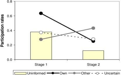
Of course, senders have two possibilities to participate. Table 3 and Figure 3 show participation rates in each of the two stages.20
20
FIGURE 3A:SENDERS’ PARTICIPATION AT STAGES 1 AND 2 IN IP.
0.0 0.2 0.4 0.6 0.8
Stage 1 Stage 2
P
a
rt
ic
ipa
tion r
a
te
s
Uninformed Own Other Uncertain
FIGURE 3B:SENDERS’ PARTICIPATION AT STAGES 1 AND 2 IN IS.
0.0 0.2 0.4 0.6 0.8
Stage 1 Stage 2
P
a
rt
ic
ipa
tion r
a
te
s
Uninformed Own Other Uncertain
RESULT 5: Senders attempt to influence their neighbor. If the receiver is an ally,
senders mainly vote at stage 1. If the receiver is an adversary, senders participate more at stage 2.
For other, we observe the opposite: senders’ participation rates are lower at stage 1 than at stage 2 (28% vs. 43% in IP; 39% vs. 43% in IS). The difference is significant (5%-level, one-tailed Wilcoxon signed ranks test) for IP, but not for IS (at the 10% level). In
uncertain, senders participate at a higher rate at stage 1 than at stage 2 (37% vs. 28% in IP; 37% vs. 30% in IS), but the differences are much smaller than in own and insignificant at the 10% level.
Note that ‘senders’ in US have higher participation rates at stage 1 than at stage 2 (38%
vs. 12%). This holds for all ‘information conditions’ in each electorate. In fact, at stage 1 they participate at the same rate as senders in other or uncertain do when information is exchanged. This appears to imply that there is a tendency to participate at a base rate of 30-40% by senders at stage 1, unless they are matched with an ally, in which case their turnout is almost twice as high. In the absence of information, receivers participate at approximately this base rate as well. At stage 2, the ‘uninformed’ base rate is at approximately 10-15%. In own and uncertain, senders participate at somewhat higher rates than this, but the most noticeable fact is that senders whose neighbors are adversaries vote at a much higher rate (43%) at stage 2, when their decision is not observed.
The participation levels of senders and their patterns of behavior are similar for partners and strangers. In this respect, neither our conjecture that participation is higher in partners nor that information exchange is more important in strangers is supported for senders. However, senders are trying to influence their receiver-neighbors. If their choices have different effects on receivers in partners than in strangers, there may be an indirect effect of senders’ behavior on the role of information exchange. We will discuss this in the next subsection. Here, we close with a result for the comparative statics. The equilibrium prediction is H3, that senders’ turnout rates are higher at stage 2 than at stage 1. Result 5 shows that this is rejected for allies.
4.5RECEIVER BEHAVIOR
RESULT 6: Receivers participate at a higher rate in partners than in strangers.
Contrary to senders, receivers behave differently in partners and strangers. Their turnout is lower in the latter case (59% vs. 52%); both are substantially higher than the 31% in US (cf. table 3). One-tailed Wilcoxon-Mann-Whitney tests reject the null hypothesis of no differences in favor of higher rates for receivers in both informed than in uninformed (1% significance level) and in IP than IS (10%-level). This holds for all information conditions and for both observed decisions of their sender-neighbors (the only exception is receiver turnout after observing a vote in other). Moreover, aggregate participation by receivers is lower than by senders in IS (cf. result 4).
RESULT 7: Receivers reciprocate allied senders’ stage 1 decisions in strangers.
The average participation rate in the uninformed sessions is 31% (cf. table 3). In IP, responses to senders’ stage 1 decisions vary: participation rates after observing a sender vote are equal to those after abstention in own (63% vs. 62%), they are lower in other
(52% vs. 59%), and higher in uncertain (66% vs. 53%). Only the latter difference is statistically significant at the 10%-level (one-tailed Wilcoxon signed ranks tests). In IS, we always observe higher participation rates after senders participate than when abstention is observed (own: 59% vs. 43%; other: 56% vs. 51%; uncertain: 58% vs. 47%). Wilcoxon signed ranks tests reject the null of no difference for own and uncertain
at the 10%-level (one-tailed tests), but cannot reject it for other.
Finally, consider the last two comparative statics predictions of section 3. H4 predicts that receivers respond to observed abstention by participating more. This is rejected by our data, especially for the strangers treatment. H5 compares receivers’ responses to an observed vote and predicts a higher turnout for receivers-adversaries. Table 3 rejects this prediction: in both IP and IS, receivers vote more after seeing an ally vote than after participation by an adversary.
4.6EFFICIENCY AND EARNINGS
Efficiency can easily be measured in the NIE participation game, because groups are of equal size. In all cases the sum of revenues is the same, independent of participation and which group wins. Any participation is costly. Hence, efficiency requires that nobody participates. With our parameters, the efficient sum of earnings per round is
30 1 6 4
6× + × = . The efficiency of an allocation is now simply defined as the sum of actual round earnings divided by 30. In addition, the lowest efficiency possible occurs when everyone votes. In this case, earnings are 6×3+6×0=18, so the minimum efficiency is 60% in this participation game. Of course, realized efficiency is inversely related to aggregate turnout. Because of the high participation in both informed treatments, average efficiency is relatively low at 76% in IP and 77% in IS. In US it is 85%. It follows directly from results 1 and 2 that the differences between informed and uninformed are statistically significant.
As for earnings, we know from result 4 that senders vote at a higher rate than receivers. Because the number of senders and receivers in the winning (and losing) groups are always equal, a direct implication is that senders earn less than receivers do. Finally, we consider the distributions of earnings for the various treatments. These are plotted in figure 4.
FIGURE 4:EARNING DISTRIBUTION PER TREATMENT.
0,0 0,1 0,2 0,3 0,4
<100 100-119 120-139 140-159 160-179 180-199 200-219 220-239 240-259 260-279 >=280
Earning categories (in tokens)
P
ro
p
o
rt
io
n
IP IS US
dination happens particularly within-groups, leading to situations where one group in an electorate wins more often than the other. 21 Hence, the weaker group is represented by the left peak in figure 4 and the stronger group by the right peak.22
4.7INTERPRETING THE RESULTS
Our collection of results appears to be quite divers. In this subsection, we try to put the pieces of the puzzle together to obtain a general picture of the effect of neighborhood information exchange on participation. We do so by formulating a conjecture of what is taking place in our experiment. Keeping in mind that what we present is indeed no more than a conjecture, we note that the processes described can account for results 1-7 and for our conclusions with respect to H1-H5. For completeness’ sake, we summarize these results in table 4.
The core of our conjecture is the implicit coordination between subjects.23 This may take various forms in our experiment. A first distinction is between coordination at the neighborhood- and group-levels. A second distinction is between intra- and inter-group
21
The victory rate of the weaker group is always smaller in IP than in IS, resulting in a rejection of the null hypothesis that there is no difference (one-tailed Wilcoxon-Mann-Whithney test, 1% significance level).
22
TABLE 4:AN OVERVIEW OF THE RESULTS
Empirical results Equilibrium comparative statics
R1: NIE increases turnout
R2: Partners/strangers has no overall effect R3: Turnout is highest in own, lowest in uncertain
R4: Senders participate more than receivers R5: Allied senders participate at higher rates at stage 1; Adversary senders participate at higher rates at stage 2
R6: Receivers vote more in partners than in strangers R7: Receivers reciprocate allied senders’ stage 1 decisions in strangers (not in partners)
H1: Turnout is higher for adversaries than for allies: rejected
H2: Allied senders vote more than receivers: accepted
H3: Senders participate at higher rates at stage 2: rejected for allies, accepted for adversaries
H4: Receivers participate more after observing abstention: rejected
H5: Adversary receivers participate more after observing a vote than allied receivers: rejected
coordination. Within groups, coordination is to higher levels of participation, in order to ‘beat’ the other group. Between groups, coordination aims at reducing participation in order to decrease costs (i.e., increase efficiency). Recall that Schram and Sonnemans (1996b) and Goren and Bornstein (2000) report an increase in participation when within-group communication is introduced. Both studies use partners. The communication allows for explicit, though not binding, coordination at the group level. In essence, their result suggests that intra-group coordination (towards participation) dominates inter-group coordination (towards abstention). We will see that the same holds for the implicit
coordination through NIE in our experiment.
Introducing NIE gives neighbors the opportunity to (implicitly) coordinate in both, partners and strangers. On the other hand, (implicit) coordination at the group level can arise across rounds in partners, but not in strangers. As a consequence, we predicted the relative importance of NIE to be lower in partners than in strangers. Therefore, we distinguish between the ways in which NIE works in both treatments.
Our major finding holds for both, partners and strangers, however: NIE substantially increases overall participation. This indicates that interaction within neighborhoods has a strong effect per se. For strangers, this follows directly from a comparison between IS and US (58% vs. 38%; cf. result 1). For partners, we note that Schram and Sonnemans (1996a) report an average turnout of 42% without NIE, which is much lower than the observed 61%-points here (cf. figure 1).
23