ISSN 1546-9239
© 2005 Science Publications
Corresponding Author: Yusaf T. F., Department of Mechanical Engineering, Universiti Tenaga Nasional, Km 7, Jalan Kajang-Puchong, Kajang, Selangor 43009, Malaysia
Modeling of Transient Heat Flux in Spark Ignition Engine
During Combustion and Comparisons with Experiment
Yusaf, T.F., Sye Hoe, Fong, M.Z. Yusoff and I. Hussein
Department of Mechanical Engineering, Universiti Tenaga Nasional, Km 7,
Jalan Kajang-Puchong Kajang, Selangor 43009, Malaysia
Abstract: A quasi-one dimensional engine cycle simulation program was developed to predict the transient heat flux during combustion in a spark ignition engine. A two-zone heat release model was utilized to model the combustion process inside the combustion chamber. The fuel, air and burned gas properties throughout the engine cycle were calculated using variable specific heats. The transient heat flux inside the combustion chamber due to the change in the in-cylinder gas temperature and pressure during combustion was determined using the Woschni heat transfer model. The program was written in MATLAB together with the Graphical User Interface (GUI). Numerical results were compared with the experimental measurements and good agreement was obtained. Four thermocouples were used and positioned equi-spaced at 5mm intervals along a ray from the spark plug location on the engine head. These thermocouples were able to capture the heat flux release by the burned gas to the wall during the combustion process including the cycle-to-cycle variations. Pressure sensor was installed at the engine head to capture the pressure change throughout the cycle.
Key words: Internal combustion engine, Woschni, spark ignition engine, heat flux, mathematical model
INTRODUCTION
Heat transfer between the working fluid and the combustion chamber in the internal combustion engine is one of the most important parameters for cycle simulation and analysis. Heat transfer influences the in-cylinder pressure and temperature levels, engine efficiency and exhaust emissions. During the combustion process, the peak gas temperature was limited to 2500K as metal components of the combustion chamber can only withstand 600K for cast iron and 500K for aluminum alloys. Therefore, the cooling of the cylinder head, block and piston is very important to keep the engine running in optimum condition. The engine lubricant will oxidize if the temperature reaches more than 450K. Thus, investigating the transient heat flux in the cylinder is very significant. The quasi one dimensional model was acceptable since the temperature gradient normal to the wall is large compared with the temperature gradients along the wall[1].
Numerical analysis: In order to determine the transient heat flux inside the combustion chamber during the combustion process, the heat transfer need to be defined as a function of θ as shown in the following equation[2]:
l b u
dQ Q Q Q
d
− − −
= =
θ ω ω
ɺ ɺ ɺ
(1)
The combustion gases are defined into two zones which are unburned gas zone and burned gas zone where Qɺb and Qɺu are the heat transfer rates for the
burned and unburned gas respectively. The heat fluxes for both burned and unburned gases were expressed as functions of temperatures as follows:
(
)
b b b w
Qɺ =hA T −T (2)
(
)
u u u w
Qɺ =hA T −T (3)
where, Ab and Au are the areas of the burned and unburned gas in contact with the cylinder walls at temperature Tw. The wall temperature is assumed to be 450K which is the maximum allowable limit for the lubricating oil to work under a proper condition before it oxidize due to overheat. The cylinder area inside the combustion chamber is:
2
1/ 2 b
b 4V
A x
2 b
π
= +
(4)
Likewise for unburned gas: 2
1/ 2 u
b 4V
A 1 x
2 b
π
= + −
(5)
1439 The burned gas always occupies a larger volume fraction of the cylinder. Equation (2) and (3) represent the remaining parameter, that required to determine the heat transfer coefficients. In the present work, the heat transfer coefficients are evaluated using Woschni heat transfer model[3]:
0.2 0.8 0.8 0.55 c
h =3.26B− p w T− (6)
Where: b = Bore p = Pressure T = Temperature
w = Average cylinder gas velocity
The average gas velocity is always assumed to be proportional to the mean piston speed during the intake, compression and exhaust stroke. However, during the combustion process, the gas velocity is a function of density due to temperature and pressure rise. Thus, the average gas velocity is:
(
)
d r
1 p 2 m
r r V T
w C S C P P
P V
= + −
(7)
Where: d
V = Piston displacement p
S = Mean piston speed r
T = Reference temperature r r
p , V = Pressure and volume at initial condition m
p = Motored pressure 1
C =2.28, C2=0.0during the compression stroke 1
C =2.28, C2=0.00324 during the combustion and expansion stroke
In order to determine the average gas velocity, the pressure and temperature histories throughout the cycle are required. Both of these parameters are functions of thermodynamic properties. Based on the first law of thermodynamics[2]:
U Q W
∆ = − (8)
where, the change of internal energy of any system is equal to the difference between the heat transfer and work generated by the system. The above equation can be expressed in differential form and when applied to a control volume encasing the cylinder content, the equation becomes:
1 1 du dm dQ dV m h
m u P
dθ+ dθ = dθ− dθ− ω
ɺ
(9)
Where: 1
mɺ = Mass flow rate 1
h = Enthalpy of the blow by masses u= Internal energy
Q= Heat transfer p= Pressure V= Volume
θ= Crank angle
ω= Engine speed
Thermodynamic properties
Specific internal energy: Since the thermodynamic properties change with respect to temperature and pressure, two MATLAB subroutines were programmed to return the thermodynamic properties throughout the engine cycle. The unburned routine was used to calculate the fuel-air-residual gas mixture using low temperature combustion modelling. The internal energy, enthalpy and specific heats are function of pressure and temperature. On the other hand, in the
burned routine, ten combustion species were tracked during the combustion process using chemical equilibrium combustion model. Both of these routines return partial derivatives in logarithmic form, which are required in the subsequent calculations. The specific internal energy of the system is given[2]:
(
)
b u
U
u xu 1 x u
m
= = + − (10)
Since there are two combustion zones inside the cylinder, x represents the mass fraction of the burned gas, ub is the internal energy of the burned gas at a temperature Tb and uu is the internal energy of the unburned gas at a temperature Tu. The internal energy of the burned gas is a function of both temperature and pressure:
(
)
b b b
u =u T , P (11)
and the derivatives will be:
b b b b
b
du u dT u dP
d T d P d
∂ ∂
= +
θ ∂ θ ∂ θ (12)
by substituting the logarithmic form of partial derivatives return by the burned routine[2]:
b b b b b b
Pb b
b b b
du Pv ln v dT ln v ln v dP
c v
d T ln T d ln T ln P d
∂ ∂ ∂
= − − +
θ ∂ θ ∂ ∂ θ (13)
and for the unburned gases:
u u u u u u
Pu u
u u u
du Pv ln v dT ln v ln v dP
c v
d T ln T d ln T ln P d
∂ ∂ ∂
= − − +
θ ∂ θ ∂ ∂ θ (14)
Equation (10) can be expressed in derivative form as follows:
(
)
(
)
b u
b u
du du du dx
m x 1 x u u m
d d d d
= + − + −
Substituting equations (13) and (14) into Eq. 15:
(
)
b b b
Pb
b b
u u u
Pu
u u
du Pv ln v dT
m mx c
d T ln T d
Pv ln v dT m 1 x c
T ln T d
∂
= − +
θ ∂ θ
∂
− −
∂ θ
(16)
(
)
b b u u
b u
b u
ln v ln v ln v ln v dP
mxv m 1 x v
ln T ln P ln T ln P d
∂ ∂ ∂ ∂
− + + − +
∂ ∂ ∂ ∂ θ
(
b u)
dx m u u
d
+ −
θ
This equation defined the first term on the left hand side of equation (9).
Specific volume: The specific volume of the system can be expressed in a similar manner as the specific internal energy[2]:
(
)
b u
U
v xv 1 x v
m
= = + − (17)
and the function form will be:
(
)
b b b
v =v T , P (18)
The derivatives are:
b b b b
b
dv v dT v dP
d T d P d
∂ ∂
= +
θ ∂ θ ∂ θ (19)
by substituting the logarithmic form partial derivatives return by the burned routine:
b b b b b b
b b
dv v ln v dT v ln v dP d T ln T d P ln P d
∂ ∂
= +
θ ∂ θ ∂ θ (20)
and for the unburned gas:
u u u u u u
u u
dv v ln v dT v ln v dP d T ln T d P ln P d
∂ ∂
= +
θ ∂ θ ∂ θ (21)
Likewise, equation (17) becomes:
(
)
(
)
b u
b u 2
1 dV V dm dv dv dx
x 1 x v v
m dθ −m dθ = dθ + − dθ + − dθ (22) Substituting equations (20) and (21) into equation (22) yields:
(
)
b b b u u u
b b u u
1 dV VC v ln v dT v ln v dT
x 1 x
m d m T ln T d T ln T d
∂ ∂
+ = + −
θ ω ∂ θ ∂ θ (23)
(
)
(
)
b b u u
b u
b b
v ln v v ln v dP dx
x 1 x v v
P ln P P ln P d d
∂ ∂
+ + − + −
∂ ∂ θ θ
Entropy: The entropy was expressed in a functional form where[2]:
(
)
u u u
s =s T , P (24)
And the derivatives are:
u u u u
u
ds s dT s dP
d T d P d
∂ ∂
= +
θ ∂ θ ∂ θ (25)
Substituting the logarithmic form partial derivatives return by the unburned routine yields:
u p
u u u u
u u u
C
ds dT v ln v dP
d T d T ln T d
∂
= −
θ θ ∂ θ (26)
The entropy of unburned gas was taken into account from the unburned gas was treated as an open system losing mass due to leakage and during the combustion process. Moreover, the compression stroke is no longer defined as isentropic compression.
Enthalpy: During the process of engine running, some of the mass will be lost due to blow by past the piston rings. This loss in mass will cause enthalpy losses well and will decrease engine performance. Before the combustion process, unburned gas leaks past the piston rings and after the combustion process, the burned gas also leaks past the piston rings. These losses need to be taken into account in the calculation in order to obtain accurate results. In order to relate the enthalpy loss between unburned and burned gases, mass fraction is used to represent the composition as follows[2]:
(
2)
2l u b
h = −1 x h +x h (27)
Likewise the enthalpy can be written in a functional form:
(
)
b b b
h =h T , P (28)
And for unburned gas:
(
)
u u u
h =h T , P (29)
The specific enthalpies for both burned and unburned gases were computed by the subroutines
burned and unburned and return the values for the further calculations throughout the engine cycle. As mentioned earlier, this program utilized a variable specific heat calculation and the specific heat is assumed to follow a polynomial equation as follows[3]:
p 2 3 4
1 2 3 4 5
C
a a T a T a T a T
R = + + + + (30)
where, R is the gas constant and a is the curve fitted polynomial coefficients. Thus, since p
p h
C T
∂
=
∂
, by
1441 Mass blow by pass rings: The rate of change of mass with respect to crank angle is represented in equation (9). By considering the mass conservation equation and considering the mass lost due to the blow by past the piston rings, the rate of change of mass with respect to crank angle can be written as follows[2]:
dm m Cm
d
− −
= =
θ ω ω
ɺ
(31)
where, ω is the engine rotational speed and the constant C is dependent on the ring design inside the engine. If the total mass loss is assumed to be 2.5%, the coefficient is 0.8.
Burn fraction, mass and volume of the system: The burn fraction was expressed in three different phases, compression, combustion and expansion[3].
Before the ignition/compression:
x=0 (32)
During the combustion:
s
b 1
x 1 cos 2
πθ − θ
= −
θ
(33)
After the combustion/expansion:
x=1 (34)
were, θs is the spark timing and θb is the burn duration. The mass at any crank angle is assumed to be given by:
(
)
1 1
m=m exp− θ − θC /ω (35)
where, m1 is the mass at the start of the compression stroke assumed to be 180° before top dead center (BTDC) and θ1 is 180° BTDC. The cylinder volume is given by:
1/ 2 2
2
d
V 1 1 l l
1 cos sin
V r 1 2 a a
= + + − θ − − θ
− (36)
where, r is the compression ratio, ε is stroke to rod length ratio s
2l
and Vd is volume at top dead center. Solution procedure: It can be seen from equation (9) that all terms had been investigated and the only term left is the work term. The work done by the piston is equal to the product of pressure and the volume change with respect to crank angle. Solving the last term will give the output of pressure, temperature of burned gas, temperature of unburned gas, work done, heat loss and the enthalpy loss change with respect to crank angle[2]:
(
)
1 b u
dP
f , P,T ,T
dθ= θ (37)
(
)
b
2 b u
dT
f , P,T ,T
dθ = θ (38)
(
)
u
3 b u
dT
f , P,T ,T
dθ = θ (39)
Since the work done, heat loss and enthalpy are related to the pressure, temperature of burned gas and unburned gas, simultaneous integration of all the above equations will give the pressure, temperature of burned gas, temperature of unburned gas, work done, heat loss and the enthalpy loss change throughout the engine cycle:
( )
4 dW
f , P
dθ = θ (40)
(
)
l
5 b u
dQ
f , P,T ,T
dθ = θ (41)
(
)
l
6 b u
dH
f , P,T ,T
dθ = θ (42)
However, in order to solve the equations above, another equation need to be derived based on the thermodynamic properties. The unburned gas was treated as an open system losing heat (Q) due to the mass transfer and the irreversibility such as mixing:
(
)
uu u
ds Q m 1 x T
d
− = ω − θ
ɺ (43)
Substituting equation (26) into equation (43) to eliminate dsu
dθ gives:
(
)
(
) (
)
u 2 1/ 2 u up u u w
u
b 4V
h
1 x
2 b
dT ln v dP
c v T T
d ln T d m 1 x
π
− + −
∂
− = −
θ ∂ θ ω − (44)
Thus, equation (9), (23) and (44) yields the solutions for an equation (37), (38) and (39). The six equations are then integrated by using the ode45
function in MATLAB. The ode45 uses the Runge-Kutta integration to integrate the ODEs[2]:
dP A B C
d D E
+ + =
θ + (45)
( )
b b
2
1/ 2 u w
b b b
P P b
b 4V
h x T T
2 b
dT v ln v A B C
d mc x c ln T D E
π
− + −
∂ + +
= +
θ ω ∂ +
(
)
b
2 u b
P
h h dx C
x x xc d
−
+ − −
θ ω
(46)
(
)
( ) ( ) u u 2 1/ 2 u wu u u
P P u
b 4V
h 1 x T T
2 b
dT v ln v A B C
d mc 1 x c ln T D E
π
− + − −
∂ + +
= +
dW dV P
dθ = dθ (48)
(
)
(
)
(
)
2
1/ 2 1/ 2
l
b u u w
dQ h b 4V
x T T 1 x T T
d 2 b
π
= + − + − −
θ ω (49)
(
2)
2l
u b
dH Cm
1 x h x h d
= − +
θ ω (50)
Where: 1 dV VC A
m d
= +
θ ω
(51)
b 2
1/ 2
b b b w
P b b
b 4V
2 b v ln v T T
B h ( x
m c ln T T
π +
∂ −
=
ω ∂
(
)
u
1/ 2
u u u w
P u u
v ln v T T
1 x )
c ln T T
∂ −
+ −
∂ (52)
(
)
(
)
b
2 b u b
b u b
b P b
x x C dx ln v h h dx
C v v v
d ln T c T d
−
∂ −
= − − − −
θ ∂ θ ω (53)
b
2 2
b b b b
P b b
v ln v v ln v D x
c T ln T P ln P
∂ ∂
= +
∂ ∂
(54)
(
)
u
2 2
u u u u
P u u
v ln v v ln v E 1 x
c T ln T P ln P
∂ ∂
= − +
∂ ∂
(55)
Equation (45) and (46) are the main focus of this study. Both pressure and burned temperature history was used to calculate the heat transfer coefficient by using Woschni model and compare with the experimental results. To simulate the engine cycle, some parameter was taken from the engine geometry such as bore, stroke and compression ratio. The air fuel ratio at 2180rpm, spark timing and initial pressure are taken from the experiment as the input data for the simulation.
Fig. 1: Pressure history throughout the engine cycle
The simulation was developed under no-load operating conditions. The pressure change from compression stroke to expansion was clearly shown in Fig. 1 whereas the unburned and burned gas temperature was shown in Fig. 2. Both pressure and temperature history was very useful parameter to determine the heat flux of the engine cycle. The unburned gas temperature was usually referred to the residual gas whereby the burned gas temperature was referring to the gaseous burning during the combustion.
Experimental investigation
Engine test bed: The engine used for this investigation at the laboratories of University of Southern Queensland was a single cylinder four stroke Briggs and Stratton, model 92232, type 1245E1, 3.5hp vertical shaft, bore 65mm, stroke 44mm, compression ratio 6 and displacement volume of 146cm3. The main bearings are oil lubricated and the engine is air-cooled. To avoid the rotating magnetic field by the magneto ignition system interfering with the heat flux measurement, the ignition system was replaced with an electronic system. The pressure transducer and heat flux gauges installed in the cylinder head as shown in Fig. 3. The wires were passed through a hole drilled through the cylinder head and connected to the charge amplifier before it goes into the data acquisition system. The engine was operated at approximately 2180rpm without any loading apart from frictional losses and windage. A once per revolution signal from an infrared shaft encoder was used to identify the engine speed. The spark timing was also set relative to the signal from the shaft encoder, which is 10.7º BTC[4].
Coaxial surface junction K-type thermocouple was constructed “in-house” by University of Southern Queensland as described[5] and used for temperature measurement. The thermocouple junctions were constructed by using 120 abrasive grit were based on previous calibration work, the 120 grit or finer gives faster response less than 1µs. These thermocouples were installed at the engine head with epoxy which serves as an electrical insulator for the thermocouples. In order to determine the fluctuations in heat flux from the transient surface junction thermocouple measurements, the “thermal product” needs to be known.
1443 Fig. 3: Illustration of the pressure transducer and
thermocouple location
The “thermal product was defined as ρck where ρ is the density, c is the specific heat and k is the thermal conductivity. From the previous calibration work, the effective thermal product of the gauges was taken as 9000J/m2Ks1/2. The signals from thermocouples were amplified with a gain of 500 and then conditioned using electrical analogue units as described[6]. The voltage signal from this analogue units, pressure transducer and the crank angle encoder were recorded using two digital oscilloscopes (Tektronix TDS420A). Each signal was recorded at either 100kSamples/s or 5kSamples/s with a total of 30k samples for each signal. The in-cylinder pressure was measured by a commercial quartz pressure transducer (PCB mode number 112B11) and an in-line charge amplifier (PCB model number 402A03) was used. The pressure transducer was set to have a sensitivity of 0.153mV/kPA for temperature lower than 300°C.
Experimental results: Figure 4b, c, d, e and f show the heat flux cycle of each thermocouple. The arrow sign indicated the cold structure occurred during the combustion. The heat flux was recorded by tc1 before tc2, tc3 and tc4 since it placed just beside the spark plug. Figure 4b shows the significant rises of heat flux of tc1 and tc2 whereas tc3 and tc4 have significant decay of it. The pressure of each consecutive cycle appears to be similar where fig. 4a shows the pressure as a change relative to the lowest value measured in the cycle. The peak pressure difference was about 350kpa, which is relatively low.
a) Pressure-cycle 1-5
b) Heat flux-cycle 1
c) Heat flux-cycle 2
d) Heat flux-cycle 3
e) Heat flux-cycle 4
f) Heat flux-cycle 5
Fig. 5: Heat flux vs. crank angle
RESULTS AND DISCUSSION
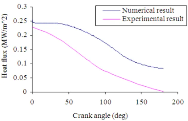
The mathematical model was developed based on the variation of thermodynamic properties calculations. The thermodynamic properties that used in this model were put in empirical function, where x value represents the mass fraction of the burnt cylinder content. Practically,
x
has left as a parameter to be determined from experiments, otherwise more complicated scheme may be used based on the assumption of the flame shape. Since the mass fraction differentiate the burned and unburned gas region, the value of x has a significant effect on the accuracy of the results. The temperature history that obtained from the simulation was used in equation (2) and (3) in order to determine the heat flux of unburned and burned gas regions. In this case, the burned gas region was only used to be compared with the experimental result since the heat flux was recorded during the combustion phase only. The simulation was in one dimension and this is acceptable due to the gradient normal to the wall is large compared with the temperature gradient along the wall. Moreover, the temperature differences along the wall decay rapidly since the epoxy seal serves as an insulator to the thermocouple body. A 100 of consecutive heat flux cycles during combustion was simulated and plotted to be compared with the experimental data. In order to obtain closed practical results, engine specifications such as bore, stroke, spark timing, rpm, compression ratio and ignition timing should be used as an input data for this mathematical model. The experimental heat flux was found to be slightly lower than numerical one. The heat flux losses can consider zero as the calculation considered the flam as adiabatic flame Nevertheless, the trend of the graph is still similar to the experimental results. The pressure and heat flux do not increase significantly during combustion the rate of the heat release due to combustion is slow, also the volume increases rapidly at he same time.Figure 5 shows the average heat flux cycles of the burned gases during the combustion and the expansion, however compression stroke has not considered in this
case. This is to match with the experimental result from University of Southern Queensland that was presented to the burned gas region only[4].
CONCLUSION
The mathematical model was proven very good agreement with the experimental results in term of heat flux and pressure rise during combustion stroke. It was found that the trend of the heat flux curve for both result are having the same pattern. The difference between the numerical and experimental result was due to the theoretical assumptions of mass fraction for burned and unburned gas region. Moreover, the temperature gradient along the wall was ignored since the mathematical model was one dimensional model. Although the temperature gradient is not that significant but still it can cause minor difference from the experimental outcome. This model can significantly contribute to play very significant role to determine the net heat flux inside the combustion chamber for different type of gaseous fuel. Application wise, the model can be very helpful tool to investigate the quality of combustion in the combustion chamber.
ACKNOWLEDGMENT
The author would like to thank Dr. Butts worth from the University of Southern Queensland for providing the experimental data.
REFERENCES
1. Oude Nijeweme, D.J., J.B.W. Kok, C.R. Stone and L. Wyszynski, 2001. Unsteady in-cylinder heat transfer in a spark ignition engine: Experiments and modelling. Proc. Instn Mech. Engrs. Part D, J. Automobile Engg., 215: 747-760.
2. Colin R. Ferguson, 1986. Internal Combustion Engines- Applied Thermo Sciences. John Willey & Sons.
3. John B. Heywood, 2003. Internal Combustion Engine Fundamentals. McGraw-Hill, pp: 371-470. 4. David, R. Butts worth and C. Matthew Wright,
2004. Observations of combustion in a spark ignition engine using transient heat flux measurements. 7th Aus. Heat and Mass Transfer Conf.
5. Butts worth, D.R. and P.A. Jacobs, 1998. Total temperature measurements in a shock tunnel facility. 13th Aus. Fluid Mechanics Conf., 1: 51-54.
![Fig. 4a-f: Pressure and heat flux from 5 consecutive cycles [6]](https://thumb-eu.123doks.com/thumbv2/123dok_br/18279419.345436/6.918.526.757.82.1070/fig-a-f-pressure-heat-flux-consecutive-cycles.webp)