<sup>10</sup>Be in late deglacial climate simulated by ECHAM5-HAM – Part 2: Isolating the solar signal from <sup>10</sup>Be deposition

(1)

CPD

9, 5627–5657, 2013

10_{Be in deglaciation –}

Part 2: Isolating solar signal

U. Heikkilä et al.

Title Page

Abstract Introduction

Conclusions References

Tables Figures

◭ ◮

Back Close

Full Screen / Esc

Printer-friendly Version

Interactive Discussion

Discussion

P

a

per

|

D

iscussion

P

a

per

|

Discussion

P

a

per

|

Discuss

ion

P

a

per

|

Clim. Past Discuss., 9, 5627–5657, 2013 www.clim-past-discuss.net/9/5627/2013/ doi:10.5194/cpd-9-5627-2013

Open Access

Climate of the Past

Discussions

This discussion paper is/has been under review for the journal Climate of the Past (CP). Please refer to the corresponding final paper in CP if available.

10

_{Be in late deglacial climate simulated by}

ECHAM5-HAM – Part 2: Isolating the solar

signal from

10

Be deposition

U. Heikkilä1, X. Shi2, S. J. Phipps3, and A. M. Smith1

1

Australian Nuclear Science and Technology Organisation (ANSTO), Lucas Heights, NSW, Australia

2

Centre for Atmospheric Chemistry, University of Wollongong, NSW, Australia

3

ARC Centre of Excellence for Climate System Science and Climate Change Research Centre, University of New South Wales, Australia

Received: 6 September 2013 – Accepted: 19 September 2013 – Published: 15 October 2013

Correspondence to: U. Heikkilä (ulla.heikkilae@eawag.ch)

(2)

CPD

9, 5627–5657, 2013

U. Heikkilä et al.

Title Page

Tables Figures

◭ ◮

Back Close

Full Screen / Esc

Discussion

P

a

per

|

D

iscussion

P

a

per

|

Discussion

P

a

per

|

Discuss

ion

P

a

per

|

Abstract

This study investigates the effect of deglacial climate on the deposition of the so-lar proxy 10Be globally, and at two specific locations, the GRIP site at Summit, Central Greenland, and the Law Dome site in coastal Antarctica. The deglacial cli-mate is represented by three 30 yr time slice simulations of 10 000 BP (years before

5

present=1950 CE), 11 000 BP and 12 000 BP, compared with a preindustrial control simulation. The model used is the ECHAM5-HAM atmospheric aerosol–climate model, driven with sea surface temperatures and sea ice cover simulated using the CSIRO Mk3L coupled climate system model. The focus is on isolating the 10Be production signal, driven by solar variability, from the weather or climate driven noise in the10Be

10

deposition flux during different stages of climate. The production signal varies on lower frequencies, dominated by the 11 yr solar cycle within the 30 yr time scale of these ex-periments. The climatic noise is of higher frequencies. We first apply empirical orthogo-nal functions (EOF) aorthogo-nalysis to global10Be deposition on the annual scale and find that the first principal component, consisting of the spatial pattern of mean10Be deposition

15

and the temporally varying solar signal, explains 64 % of the variability. The following principal components are closely related to those of precipitation. Then, we apply en-semble empirical decomposition (EEMD) analysis on the time series of10Be deposition at GRIP and at Law Dome, which is an effective method for adaptively decomposing the time series into different frequency components. The low frequency components

20

and the long term trend represent production and have reduced noise compared to the entire frequency spectrum of the deposition. The high frequency components rep-resent climate driven noise related to the seasonal cycle of e.g. precipitation and are closely connected to high frequencies of precipitation. These results firstly show that the10Be atmospheric production signal is preserved in the deposition flux to surface

25

(3)

avail-CPD

9, 5627–5657, 2013

U. Heikkilä et al.

Title Page

Tables Figures

◭ ◮

Back Close

Full Screen / Esc

Discussion

P

a

per

|

D

iscussion

P

a

per

|

Discussion

P

a

per

|

Discuss

ion

P

a

per

|

able data sets, or by decomposing the individual data sets to filter out high-frequency fluctuations.

1 Introduction

Reconstruction of solar activity has so far only been possible for the Holocene (e.g. Steinhilber et al., 2012; Vonmoos et al., 2006). Evidence of the existence of solar

cy-5

cles during the last ice age was found by Wagner et al. (2001) in the 10Be record from the GRIP ice core between 25 and 50 kyr BP, but a continuous record extending from the Holocene into the preceding ice age is still missing. During the last deglacia-tion the solar proxies 10Be and 14C exhibited significant, climate driven, differences, which complicates the extraction of the solar signal (e.g. Muscheler et al., 2004). In

10

order to study the climate impact on10Be during the last deglaciation we perform time slice model simulations during three stages: 10 000 (“10k”), 11 000 (“11k”) and 12 000 (“12k”) BP (years before 1950 CE), compared with a control (“ctrl”) simulation during the preindustrial climate. The mean climate change as well as the mean difference in 10

Be deposition and atmospheric distribution has been analysed in an accompanying

15

manuscript (Heikkilä et al., 2013). The main findings are that the lower greenhouse gas concentrations in the deglaciation simulations influence the climate, leading to a tropo-spheric cooling and drying and changes in sea ice cover which affect atmospheric circulation patterns. However, these changes were found to cause10Be deposition to fluctuate by no more than 50 % locally, although changes in air concentrations and dry

20

deposition were significantly larger than that. The results indicate that10Be deposition is mostly driven by mass balance. The amount of10Be produced in the atmosphere is deposited to the surface within a few years and therefore, averaged over a few years, the deposition equals production.

While the accompanying study concentrates on spatial differences as influenced by

25

(4)

CPD

9, 5627–5657, 2013

U. Heikkilä et al.

Title Page

Tables Figures

◭ ◮

Back Close

Full Screen / Esc

Discussion

P

a

per

|

D

iscussion

P

a

per

|

Discussion

P

a

per

|

Discuss

ion

P

a

per

|

deposition flux. The aim is to assess how much the production signal is distorted by climatic noise in these simulations. We first focus on global deposition and quantify the different components of the variability, production and climate-related “noise”, with the aid of empirical orthogonal function (EOF) analysis. Then, because observations do not cover the entire globe but are limited to a few locations we analyse time series of

5

the modelled10Be deposition at two locations: the GRIP drilling site in Greenland and the Law Dome site in Antarctica.

The traditional approach to detect solar cycles in 10Be records has been to cre-ate a frequency, for example a Fourier, spectrum which reveals the known solar cy-cles, e.g.∼11 (Schwabe),∼22 (Hale),∼88 (Gleissberg),∼205 (de Vries) and∼2300

10

(Hallstatt) yr (e.g. McCracken et al., 2012). Bandpass filtering has been used to dis-tinguish between solar and geomagnetic modulation of10Be production by assuming that fluctuations with frequencies below a given threshold, typically 1000 yr, are due to geomagnetic variations whereas high-frequency fluctuations are due to solar variability (Beer et al., 1994, 2002; Wagner et al., 2001). The drawback of using the Fourier

spec-15

trum to detect frequency peaks is that the length of each solar cycle is assumed to be constant in time. However, the length of the cycles has been found to be non constant and is currently under much investigation (e.g. Richards et al., 2009). Already during the 30 yr period investigated within this study each of the three ca. 11 yr cycles varies by±1 yr in length. Bandpass filtering, on the other hand, requires a priori knowledge of

20

the frequencies of the cycles to set the frequency limits. To overcome these potentially limiting assumptions we propose the ensemble empirical mode decomposition (EEMD) method (Huang and Wu, 2008; Huang et al., 1998; Wu and Huang, 2009) in this study. EEMD decomposes the10Be signal into a set of frequency components, termed intrin-sic mode functions (IMFs). As this decomposition is based on the local characteristics

25

(5)

CPD

9, 5627–5657, 2013

U. Heikkilä et al.

Title Page

Tables Figures

◭ ◮

Back Close

Full Screen / Esc

Discussion

P

a

per

|

D

iscussion

P

a

per

|

Discussion

P

a

per

|

Discuss

ion

P

a

per

|

resulting from EEMD analysis can then be combined to be associated with solar or geomagnetic forcing on10Be data.

EEMD has widely been used in time series analysis, such as surface temperature (Franzke, 2012), tree ring data (Shi et al., 2012) and changes in onset of seasons (Qian et al., 2009), but, to our knowledge, never in combination with10Be. This study focuses

5

on the level of distortion of the solar signal in10Be deposition due to deglacial climate changes. Model data is useful to test the suitability of EEMD for this study because the solar signal used is known. While the length of the model data (30 yr) restricts the type of solar cycles to be studied to only the 11 yr one, EEMD can be applied to real-world data including a larger number of cycles in the future. The only10Be observations

10

available from the last deglaciation are from the GISP2 ice core (Finkel and Nishiizumi, 1997) but their temporal resolution of 20–50 yr does not compare with the monthly resolution of this study. Holocene observations covering several solar cycles typically have an annual or longer temporal resolution. Sub-annually resolved observations are limited in length and typically include up to one 11 yr cycle only. This prohibits a direct

15

comparison with the current model data.

2 Methods

Here we only give general information on the model simulations and refer to the ac-companying paper (Heikkilä et al., 2013) for details. The model used is the atmo-spheric aerosol–climate model ECHAM5-HAM which incorporates radionuclide

pro-20

duction, transport and deposition processes. To produce deglacial climate the model is driven with sea surface temperatures and sea ice cover obtained from simulations us-ing the CSIRO Mk3L climate system model version 1.2 (Phipps et al., 2011, 2012). Each of the ECHAM5-HAM model simulations (ctrl, 10k, 11k and 12k) represents a 30 yr time slice of an equilibriated state of climate during these periods. The10Be

25

(6)

CPD

9, 5627–5657, 2013

U. Heikkilä et al.

Title Page

Tables Figures

◭ ◮

Back Close

Full Screen / Esc

Discussion

P

a

per

|

D

iscussion

P

a

per

|

Discussion

P

a

per

|

Discuss

ion

P

a

per

|

allow the results to be quantitively compared with observations. Analysis of the mean changes in climate and in atmospheric10Be transport and deposition are provided by Heikkilä et al. (2013).

We first apply the empirical orthogonal functions (EOF) analysis, also known as prin-cipal component analysis, to global10Be data in this study. This method was introduced

5

by Lorenz (1956) and has since been widely used in climate data analysis to detect pat-terns such as the North Atlantic oscillation or the Southern Annular Mode in sea level pressure data, among various others. It creates a linear combination of a number of or-thogonal spatial patterns (referred to as EOFs in this manuscript), multiplied by a time series component (referred to as PCs). Because the global10Be deposition fields

com-10

prise a temporally varying component, the production signal, but also vary spatially due to differences in the precipitation patterns and location of the stratosphere–troposphere exchange, this method seems suitable for removing noise and reducing the dimension-ality of10Be data.

The words “signal” and “noise” will be used throughout the manuscript to refer to the

15

solar variability driven atmospheric production (signal) and climate driven fluctuations (noise) in10Be deposition data. Both components typically have very distinctive time scales. The production varies on multi-year time scales, such as the 11 yr cycle. Shorter term fluctuations in the solar activity parameter cause high-frequency fluctuations in the production rate but these are e_fficiently filtered out by the atmospheric transport from

20

the stratosphere to the troposphere. Climate related changes, the largest of which is the seasonal cycle of e.g. precipitation rate, act on sub-annual time scales. Long-term trends in climatic variables are also possible but were not found during the relatively short simulations of 30 yr each. In order to decompose the10Be deposition into various frequencies we apply the EEMD method to10Be deposition and the precipitation rate at

25

(7)

CPD

9, 5627–5657, 2013

U. Heikkilä et al.

Title Page

Tables Figures

◭ ◮

Back Close

Full Screen / Esc

Discussion

P

a

per

|

D

iscussion

P

a

per

|

Discussion

P

a

per

|

Discuss

ion

P

a

per

|

a simple 25 month running mean to smooth out the seasonal cycle but only minimally reduce the length of the data set, consistent with Heikkilä et al. (2013).

The EEMD method decomposes time series into intrinsic mode functions (IMF), each of which represents a specific frequency range, and a long-term trend. The first IMF has the highest frequency and so on. The sum of these IMFs and the long-term trend

5

reproduces the original time series. The length of the time series determines the num-ber of IMFs. Our time series consist of monthly 30 yr data, smoothed with a 25 month running mean, adding up to 336 data points. This creates seven IMFs and a long-term trend. Each of the model simulations is analysed separately, because the data has to be continuous for EEMD, and then combined.

10

The EEMD analysis can be briefly summarised as follows:

1. Add white noise with a predefined noise amplitude to the data to be analysed.

2. Run EMD to decompose the data with added white noise into IMFs.

3. Repeat the above steps several times to create the ensembles.

4. The final results are obtained as ensemble means of corresponding IMFs of the

15

decomposition.

3 Results

3.1 EOF analysis of global10_{Be deposition}

In the following we analyse the temporal variability of the simulated global10Be depo-sition flux. In order to detect the solar cycle in the10Be flux it is necessary to remove

20

(8)

CPD

9, 5627–5657, 2013

U. Heikkilä et al.

Title Page

Tables Figures

◭ ◮

Back Close

Full Screen / Esc

Discussion

P

a

per

|

D

iscussion

P

a

per

|

Discussion

P

a

per

|

Discuss

ion

P

a

per

|

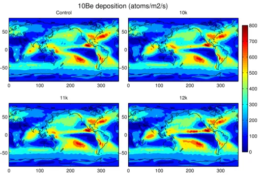
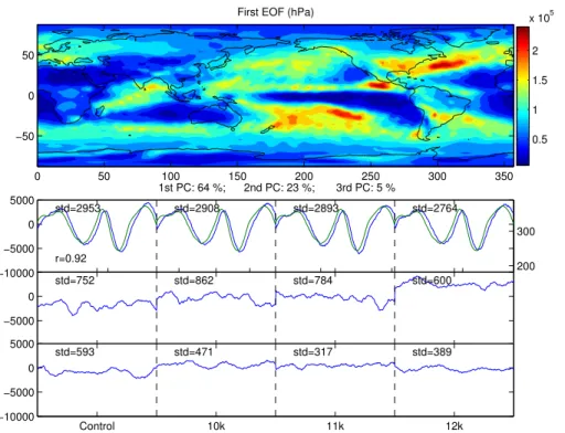
simulations combined to produce the common EOFs for each simulation. The first EOF obtained is shown in Fig. 2 together with the three first principal components. The first EOF (top panel) explains 64 % of the variability and is very similar to the mean10Be deposition pattern (Fig. 1). The first principal component, shown in blue, correlates strongly (r ₌0.92) with the 11 yr solar cycle (green). The delay of ca. 1 yr between the

5

production (solar) and the deposition signal reflects the atmospheric residence time of10Be (e.g. Beer et al., 1990). The following EOFs are fairly patternless and exhibit significant variability only in the tropics (not shown). The tropics are generally not best suited for recording 10Be as a solar proxy due to the low production variability and the uplifting of air due to the Brewer–Dobson circulation. Therefore the tropical

tropo-10

spheric air is less enriched by stratospheric10Be, which exhibits the largest production variability, and the 10Be signal in tropical tropospheric air includes more noise. The corresponding two following PCs (in blue) explain 23 % and 5 % of the variability and the rest of them less than 5 % each. It seems that the variability of the internal climate modes, described by these PCs, was not amplified in the deglaciation simulations. The

15

standard deviations (“std” shown in the figure) are slightly reduced relative to ctrl in the deglaciation simulations, especially at 12k. However the mean value of the second PC at 12k is higher.

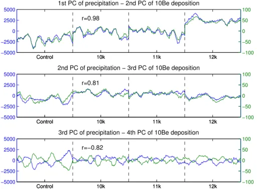
The first PC thus represents the production signal and the following PCs the climate-related noise. In order to investigate if the noise components are climate-related to climatic

20

variability we perform EOF analysis for the 25 month running mean precipitation fields. The PCs are very similar to the noise components of the10Be deposition, suggesting that the climatic noise is closely related to precipitation variability. The first three precip-itation PCs are shown in Fig. 3 (green) together with the second to fourth PCs of10Be deposition (blue). The PCs of precipitation explain 59 % (1st), 13 % (2nd) and 11 %

25

(3rd) of the variability. The correlation coefficients (0.98 to 0.81) suggest that these are closely related to the second to fourth PCs of10Be deposition.

(9)

CPD

9, 5627–5657, 2013

U. Heikkilä et al.

Title Page

Tables Figures

◭ ◮

Back Close

Full Screen / Esc

Discussion

P

a

per

|

D

iscussion

P

a

per

|

Discussion

P

a

per

|

Discuss

ion

P

a

per

|

temporally varying production signal plus noise, which can thus be discarded. Even during deglacial climate the production signal seems large enough to make full use of the method. These results suggest that this method can therefore be applied to observations as well. However, observational records might not be easily combined due to their different temporal resolution and coverage, variable quality and very limited

5

spatial coverage. In reality, insufficient observations are available to fully distinguish signal from noise.

3.2 EEMD analysis of10Be deposition at GRIP and at Law Dome

Typically these complications restrict the number of time series which can be analysed collectively. Hence, principal component analysis might not be able to reveal the solar

10

signal during periods when observations disagree. Therefore we apply an alternative method, the EEMD, to analyse time series separately at two particular locations: the GRIP site in central Greenland (72◦₃₅′_{N, 37}◦₃₈′_{W, 3216 m a.s.l.) and the Law Dome} site in coastal Antarctica (66◦46.18′S, 112◦48.69′E, 1370 m a.s.l.). Both are charac-terised by relatively high snow accumulation and therefore a number of high resolution

15

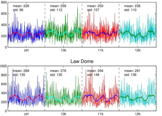
time series exist (e.g. Muscheler et al., 2005; Pedro et al., 2011; Yiou et al., 1997). We first present the modelled time series of 10Be deposition at both sites (Fig. 4) for all four simulations. Both monthly mean and 25 month running mean values are shown. The monthly fluctuations are considerable in all simulations at both stations but smoothing the seasonal cycle out (25 month running mean) reveals the solar cycle.

20

The three ca. 11 yr solar cycles are seen in all simulations at both stations, however some distortion is visible, especially at 12k. The mean value of10Be deposition only varies by ca. 5 % between these stations. While the global mean deposition has to be constant in all simulations, local changes of up to 50 % could have been expected based on the analysis of the mean climate (Heikkilä et al., 2013). The precipitation

25

(10)

CPD

9, 5627–5657, 2013

U. Heikkilä et al.

Title Page

Tables Figures

◭ ◮

Back Close

Full Screen / Esc

Discussion

P

a

per

|

D

iscussion

P

a

per

|

Discussion

P

a

per

|

Discuss

ion

P

a

per

|

reduced precipitation rate at 12k does not therefore affect the mean10Be deposition at 12k; however, it might contribute to the high amplitude of variability in the reconstructed production signal at 12k.

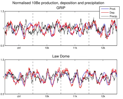
Figure 6 shows the data as input for the EEMD analysis, with the 25 month running mean10Be production, deposition and precipitation rate. The production rate shown is

5

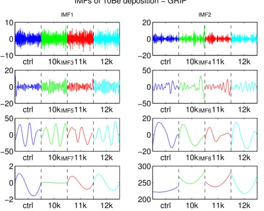
the global mean. The data is normalised through division by the mean, showing that the amplitude of the deposition variability is comparable with the global mean produc-tion rate variability. The 10Be deposition follows the three solar cycles shown by the production rate in all simulations at both stations. The 10Be deposition is delayed in exhibiting the second production minimum in the 11k simulation at GRIP, which could

10

be due to the large simultaneous peak in the precipitation rate. Given the length of the time series, the EEMD analysis results in seven intrinsic mode functions (IMFs). These are shown in Figs. 7 and 8. In addition, a long term trend is obtained (IMF8). The sum of these IMFs and the trend reproduces the original data. The first three IMFs are in-terpreted as climate-related noise as their frequency is less than annual. The following

15

five IMFs (4–8) are considered to represent the solar signal, or10Be production rate. Which IMFs are attributed to signal and noise is ambiguous and depends on the time resolution of the data. In our case, sub-annual variations can only be of climatic origin and can be discarded as noise. It might be advantageous to vary the number of the IMFs used to reconstruct the production as closely to the original solar signal as

pos-20

sible in each simulation, but in case of observations the actual signal is not known. We therefore aim to create a standard methodology based on physically justified thresh-olds which can be applied to any data without prior knowledge of the reconstructed signal.

The high-frequency components IMF1–2 do not vary significantly between the

simu-25

(11)

CPD

9, 5627–5657, 2013

U. Heikkilä et al.

Title Page

Tables Figures

◭ ◮

Back Close

Full Screen / Esc

Discussion

P

a

per

|

D

iscussion

P

a

per

|

Discussion

P

a

per

|

Discuss

ion

P

a

per

|

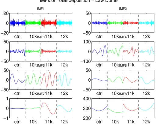
third of each 30 yr period. This suggests a stronger climatic impact on10Be deposi-tion during this period, seen as anomalously low precipitadeposi-tion rate at ctrl, 10k and 11k (Fig. 6). The IMF7 has a similar form but is flat in 10k, however its amplitude is neg-ligible compared with other IMFs. At Law Dome the noise components (IMF1–3) are fairly similar in amplitude in all simulations. IMF4 has a lower frequency in ctrl than in

5

the other simulations, and it contributes more to the two last solar cycles than IMF5, which nearly misses them. Such a shift towards higher-frequencies suggests stronger climate impact during the last solar cycle. This is consistent with the higher amplitude of the high-frequency IMFs of precipitation (not shown) which seems to distort the solar signal in10Be deposition. Also the percentage of total variability explained by noise is

10

larger at 7 % than in other simulations (see the following subsection). IMF7 is very flat in ctrl and 10k but has a distinctive pattern in 11k and 12k but again the amplitude is too small to be detected in the total signal.

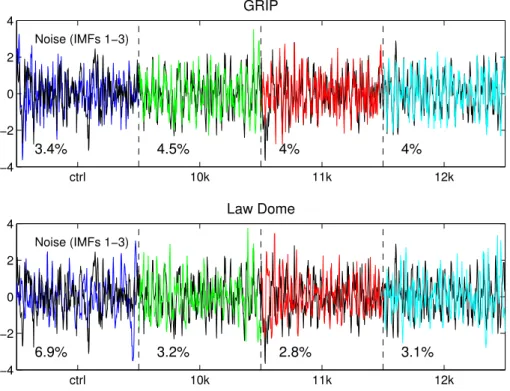
The reconstructed production signal from the10Be deposition (IMF4–8) is illustrated in Fig. 9 for both stations, together with the original production rate. Removing the

high-15

frequency noise flattens the signal and increases the agreement with production (com-pare with Fig. 6). The data sets have been normalised for comparison. The amplitude of the reconstructed production agrees reasonably well with the actual production, but is slightly underestimated at GRIP and overestimated at Law Dome in 11k. The second production maximum is underestimated in 12k at both stations. This was already seen

20

in the original data (Fig. 6) and cannot be improved by removing the high-frequency noise. Figure 10 shows the reconstructed high-frequency part of the spectrum (IMF1– 3) of both the10Be deposition and precipitation. They have been standardised to allow for comparison. Generally the variability seems similar in all simulations and both sta-tions. Both noise components seem correlated, especially in the case of 10k, 11k and

25

(12)

CPD

9, 5627–5657, 2013

U. Heikkilä et al.

Title Page

Tables Figures

◭ ◮

Back Close

Full Screen / Esc

Discussion

P

a

per

|

D

iscussion

P

a

per

|

Discussion

P

a

per

|

Discuss

ion

P

a

per

|

The variability contribution of all IMFs is shown in Fig. 11. The first three IMFs are negligible at both stations and all simulations. At GRIP, the IMF5, which is very closely related to the solar signal (see Fig. 7), explains nearly 70 % of total variability in ctrl. However, in the deglacial simulations this contribution is reduced and IMF4 and the long term trend get more weight. At Law Dome there is no single dominant IMF, but

5

IMFs 4–5 (and the long-term trend in case of deglacial simulations) are most domi-nant. Apparently IMF7, albeit exhibiting distinct differences between the simulations, is not of importance for the total variability in any of the simulations. Combining re-sults of both stations suggests that in the 12k simulation there is a significant long-term trend, which is absent in ctrl. Furthermore, the Law Dome station seems more strongly

10

a_ffected by the climatic noise than GRIP in these simulations.

In order to distinguish the effect of noise reduction from production signal we anal-yse correlations between variables. Figure 12 shows scatter plots of normalised10Be deposition and precipitation, and10Be production and deposition at GRIP.10Be depo-sition and production (signal) are shown without (IMF1–8; blue) and with (IMF4–8; red)

15

filtering of high-frequency noise,10Be deposition and precipitation (noise) only without filtering because of the di_fferent scales of the variables (IMF1–3 have zero mean due to the subtraction of the long-term mean and thus different scale). However, correlation coefficients are shown for both the unfiltered (IMF1–8; first) and the filtered (IMF1–3; second) data. Comparison of the unfiltered and filtered correlations indicates that

fil-20

tering the high-frequency noise improves the agreement between10Be deposition and production signals, however, the difference is not large. This is due to the strong 11 yr cycle which causes the data to be autocorrelated, dominating the correlation. Therefore the correlation coefficients should be interpreted as indicative only. However, we do not attempt to remove the autocorrelation because the 11 yr cycle is the very part of the

25

10

(13)

CPD

9, 5627–5657, 2013

U. Heikkilä et al.

Title Page

Tables Figures

◭ ◮

Back Close

Full Screen / Esc

Discussion

P

a

per

|

D

iscussion

P

a

per

|

Discussion

P

a

per

|

Discuss

ion

P

a

per

|

Law Dome the results are similar to GRIP. The correlation of the filtered signal with the production signal is improved from the unfiltered data, albeit only slightly. The noise components of 10Be deposition and precipitation correlate fairly strongly when unfil-tered, but the correlation is reduced when the data is filtered. This is due to a similar long-term trend, which, when filtered out, reduces the correlation. Also the fact that

5

white noise is added into the data by the EEMD might reduce the correlation between filtered data sets. Looking at Fig. 6 the precipitation rate at Law Dome seems to exhibit cycles similar in length to the 11 yr cycle, especially in ctrl and 11k. This, however, is coincidental as the model employs a standard radiation scheme with a constant value for solar irradiation. In an atmospheric-only model the climate is constrained mostly by

10

the sea-surface temperatures and sea ice and the solar irradiation plays a minor role. The physical meaning of these findings is that the temporal variability of10Be depo-sition into ice is mostly dominated by the production signal on an annual scale. The correlation between10Be deposition and production is high, but deteriorates because of fluctuations caused by short-term changes in precipitation rate. If this short-term

15

“climatic” noise is filtered out, the10Be production signal, reconstructed from the10Be deposition flux, agrees better with the actual production signal. However, this method only corrects for high-frequency noise, but cannot distinguish longer-term climatic noise from the production signal. This is shown by the fact that the excessively low or high amplitudes of the solar cycles, or the delays in the response to production minima or

20

maxima in10Be deposition, cannot be corrected for. Still, the EEMD-filtered signal ex-plains more than>95 % of total variability, a result which cannot be achieved by simple

bandpass filtering.

4 Summary and conclusions

This study analyses four time slice (30 yr each) simulations of the solar proxy10Be at

25

(14)

CPD

9, 5627–5657, 2013

U. Heikkilä et al.

Title Page

Tables Figures

◭ ◮

Back Close

Full Screen / Esc

Discussion

P

a

per

|

D

iscussion

P

a

per

|

Discussion

P

a

per

|

Discuss

ion

P

a

per

|

period (“ctrl”). We investigate to what extent the different climatic conditions distort the solar signal in the 10Be deposition flux to the surface and how the distortion can be corrected for by analysing the frequency spectrum of the 10Be deposition. The cli-matic distortion, called noise, is assumed to be represented by the highest frequencies whereas the solar signal is known to vary on a longer time scale. In order to remove

5

the seasonal cycle from the data we first smooth it using 25 month running means. First, the global field of10Be deposition is analysed to study the temporal and spatial variability by means of EOF (empirical orthogonal function) analysis, also known as PC (principal component) analysis. We find that the first spatial pattern closely resembles the global deposition field, and the first temporal pattern correlates with the solar signal

10

withr ₌0.92. 64 % of the total variability of10Be deposition can be attributed to solar, or production, variability, and 36 % to noise. Analysing the noise components we find close connections between the second and higher temporal patterns and all temporal patterns of precipitation, suggesting that precipitation variability drives the noise part of the 10Be deposition variability after the production signal has been removed. This

15

method allows for noise reduction, as the noise components can be removed. It can be applied to observational data as well, if su_fficient spatial coverage is provided and the temporal coverage matches.

As in reality the number of 10Be observations is limited, EOF analysis can pro-duce unreliable results during periods when observations disagree. We propose the

20

use of the ensemble empirical decomposition (EEMD) method, which analyses one-dimensional data. EEMD decomposes the data into intrinsic frequency components without requiring any prior knowledge of these frequencies. Furthermore, it has the ad-vantage of allowing the amplitude and the length of the cycles in the data to vary over time. We decompose the modelled10Be deposition and precipitation at two particular

25

(15)

low-CPD

9, 5627–5657, 2013

U. Heikkilä et al.

Title Page

Tables Figures

◭ ◮

Back Close

Full Screen / Esc

Discussion

P

a

per

|

D

iscussion

P

a

per

|

Discussion

P

a

per

|

Discuss

ion

P

a

per

|

frequency ones as the solar signal. The results for GRIP and Law Dome are fairly similar, and removing the high-frequency noise improves the agreement between the 10

Be deposition flux and the production signal.10Be deposition at Law Dome includes slightly more climatic noise in these simulations. The amplitude of the reconstructed production signal from the deposition is very similar to the original production.

Compar-5

ison of the noise components of 10Be deposition with those of precipitation suggests they are interconnected, in agreement with the results of the global EOF analysis.

These findings support the assumption that, regardless of the state of climate, the variability of10Be deposition is dominated by the production variability on annual and longer time scales, simply due to mass conservation. Locally significant fluctuations

10

from the global mean could have been expected but were not found, although the pre-cipitation rate was reduced in the deglacial climate. The EEMD method proved useful in analysing single data series. It was successful in noise reduction and resulted in a deposition signal closer to production, explaining >95 % of total variability in each

simulation, than can be obtained by a simple lowpass filtering or smoothing. However,

15

it was only able to remove high-frequency noise and could not correct for all spurious forms at lower frequencies. EEMD thus seems well suited for noise reduction in sin-gle10Be time series. We propose it for analysing multi-annually resolved10Be records including several solar cycles of various frequencies. Seasonal noise with its ampli-tude of several factors larger than production variability complicates the analysis of

20

high-resolved records. The strength of EEMD will be the decomposition of the entire frequency spectrum allowing for a distinction of solar cycles of various lengths, as well as the slowly varying strength of the geomagnetic field.

Acknowledgements. This work was supported by an award under the Merit Allocation Scheme on the NCI National Facility at the ANU.

(16)

CPD

9, 5627–5657, 2013

U. Heikkilä et al.

Title Page

Tables Figures

◭ ◮

Back Close

Full Screen / Esc

Discussion

P

a

per

|

D

iscussion

P

a

per

|

Discussion

P

a

per

|

Discuss

ion

P

a

per

|

References

Beer, J., Blinov, A., Bonani, G., Finkel, R. C., Hofmann, H. J., Lehmann, B., Oeschger, H., Sigg, A., Schwander, J., Staffelbach, T., Stauffer, B., Suter, M., and Wölfli, W.: Use of10Be in polar ice to trace the 11-year cycle of solar activity, Nature, 347, 164–166 , 1990. 5634 Beer, J., Baumgartner, S., Dittrich-Hannen, B., Hauenstein, J., Kubik, P., Lukasczyk, C.,

5

Mende, W., Stellmacher, R., and Suter, M.: Solar variability traced by cosmogenic isotopes, in: The Sun as a Variable Star: Solar and Stellar Irradiance Variations, edited by: Pap, J. M., Fröhlich, C., Hudson, H. S., and Solanki, S. K., Cambridge University Press, 291–300, 1994. 5630

Beer, J., Muscheler, R., Wagner, G., Laj, C., Kissel, C., Kubik, P. W., and Synal, H.-A.:

Cosmo-10

genic nuclides during isotope stages 2 and 3, Quaternary Sci. Rev., 21, 1129–1139, 2002. 5630

Finkel, R. C. and Nishiizumi, K.: Beryllium 10 concentrations in the Greenland Ice Sheet Project 2 ice core from 3–40 ka, J. Geophys. Res., 102, 26699–26706, 1997. 5631

Franzke, C.: Nonlinear trends, long-range dependence and climate noise properties of surface

15

temperature, J. Climate, 25, 4172–4183, doi:10.1175/JCLI-D-11-00293.1, 2012. 5631 Heikkilä, U. and Smith, A. M.: Production rate and climate influences on the variability of10Be

deposition simulated by ECHAM5-HAM: globally, in Greenland and in Antarctica, J. Geophys. Res., 118, 1–15, doi:10.1002/jgrd.50217, 2013. 5633

Heikkilä, U., Phipps, S. J., and Smith, A. M.: 10Be in last deglacial climate simulated by

20

ECHAM5-HAM – Part 1: Climatological influences on10Be deposition, Clim. Past Discuss., 9, 3681–3709, doi:10.5194/cpd-9-3681-2013, 2013. 5629, 5631, 5632, 5633, 5635

Huang, N. E. and Wu, Z.: A review on Hilbert–Huang transform: method and its applications to geophysical studies, Rev. Geophys. 46, RG2006, doi:10.1029/2007RG000228, 2008. 5630 Huang, N. E., Shen, Z., Long, S. R., Wu, M. C., Shih, H. H., Zheng, Q., Yen, N.-C., Tung, C.

25

C., and Liu, H. H.: The empirical mode decomposition and the Hilbert spectrum for nonlinear and non-stationary time series analysis, P. R. Soc. Lond. A Math., 454, 903–995, 1998. 5630 Lorenz, E. N.: Empirical orthogonal functions and statistical weather prediction, Science Report 1, Statistical forecasting project, Department of meteorology, MIT, NTIS AD 110268, 49 pp., 1956. 5632

30

(17)

CPD

9, 5627–5657, 2013

U. Heikkilä et al.

Title Page

Tables Figures

◭ ◮

Back Close

Full Screen / Esc

Discussion

P

a

per

|

D

iscussion

P

a

per

|

Discussion

P

a

per

|

Discuss

ion

P

a

per

|

Muscheler, R., Beer, J., Wagner, G., Laj, C., Kissel, C., Raisbeck, G. M., Yiou, F., and Ku-bik, P. W.: Changes in the carbon cycle during the last deglaciation as indicated by the com-parison of10Be and14C records, EPSL, 6973, 1–16, doi:10.1016/S0012-821X(03)00722-2, 2004. 5629

Muscheler, R., Beer, J., Kubik, P. W., and Synal, H.-A.: Geomagnetic field intensity during the

5

last 60 000 years based on10Be &36Cl from the Summit ice cores and14C, Quarternary Sci. Rev., 24, 1849–1860, doi:10.1016/j.quascirev.2005.1001.1012, 2005. 5635

Pedro, J. B., Smith, A. M., Simon, K. J., van Ommen, T. D., and Curran, M. A. J.: High-resolution records of the beryllium-10 solar activity proxy in ice from Law Dome, East Antarctica: mea-surement, reproducibility and principal trends, Clim. Past, 7, 707–721,

doi:10.5194/cp-7-707-10

2011, 2011. 5635

Phipps, S. J., Rotstayn, L. D., Gordon, H. B., Roberts, J. L., Hirst, A. C., and Budd, W. F.: The CSIRO Mk3L climate system model version 1.0 – Part 1: Description and evaluation, Geosci. Model Dev., 4, 483–509, doi:10.5194/gmd-4-483-2011, 2011. 5631

Phipps, S. J., Rotstayn, L. D., Gordon, H. B., Roberts, J. L., Hirst, A. C., and Budd, W. F.: The

15

CSIRO Mk3L climate system model version 1.0 – Part 2: Response to external forcings, Geosci. Model Dev., 5, 649–682, doi:10.5194/gmd-5-649-2012, 2012. 5631

Qian, C., Fu, C., Wu, Z., and Yan, Z.: On the secular change of spring onset at Stockholm, Geophys. Res. Lett., 36, L12706, doi:10.1029/2009GL038617, 2009. 5631

Richards, M. T., Rogers, M. L., and Richards, D. S. P.: Long-term variability in the length of the

20

solar cycle, Astr. Soc. P., 121, 797–809, doi:10.1086/604667, 2009. 5630

Shi, F., Yang, B., von Gunten, L., Qin, C., and Wang, Z.: Ensemble empirical mode de-composition for tree-ring climate reconstructions, Theor. Appl. Climatol., 109, 233–243, doi:10.1007/s00704-011-0576-8, 2012. 5631

Steinhilber, F., Abreu, J. A., Beer, J., Brunner, I., Christl, M., Fischer, H., Heikkilä, U.,

Ku-25

bik, P. W., Mann, M., McCracken, K. G., Miller, H., Miyahara, H., Oerter, H., and Wilhelms, F.: 9400 years of cosmic radiation and solar activity from ice cores and tree rings, P. Natl. Acad. Sci. USA, 109, 16, 5967–5971, doi:10.1073/pnas.1118965109, 2012. 5629

Vonmoos, M., Beer, J., and Muscheler, R.: Large variations in Holocene solar activity: con-straints from10Be in the Greenland Ice Core Project ice core, J. Geophys. Res., 111, A01015,

30

(18)

CPD

9, 5627–5657, 2013

U. Heikkilä et al.

Title Page

Tables Figures

◭ ◮

Back Close

Full Screen / Esc

Discussion

P

a

per

|

D

iscussion

P

a

per

|

Discussion

P

a

per

|

Discuss

ion

P

a

per

|

Wagner, G., Beer, J., Masarik, J., Muscheler, R., Kubik, P., Mende, W., Laj, C., Raisbeck, G. M., and Yiou, F.: Presence of the solar de Vries cycle (_∼205 years) during the last ice age, Geophys. Res. Lett., 28, 303–306, 2001. 5629, 5630

Wu, Z. and Huang, N. E.: Ensemble empirical mode decomposition: a noise-assisted data analysis method, Adv. Adapt. Data Anal., 1, 1–41, 2009. 5630

5

(19)

CPD

9, 5627–5657, 2013

U. Heikkilä et al.

Title Page

Tables Figures

◭ ◮

Back Close

Full Screen / Esc

Discussion

P

a

per

|

D

iscussion

P

a

per

|

Discussion

P

a

per

|

Discuss

ion

P

a

per

|

Control

0 100 200 300

−50 0 50

10k

0 100 200 300

−50 0 50

11k

0 100 200 300

−50 0 50

0 100 200 300 400 500 600 700 800 10Be deposition (atoms/m2/s)

12k

0 100 200 300

−50 0 50

Fig. 1.Mean10Be deposition (atoms m−2

s−1

(20)

CPD

9, 5627–5657, 2013

U. Heikkilä et al.

Title Page

Tables Figures

◭ ◮

Back Close

Full Screen / Esc

Discussion

P

a

per

|

D

iscussion

P

a

per

|

Discussion

P

a

per

|

Discuss

ion

P

a

per

|

First EOF (hPa)

0 50 100 150 200 250 300 350

−50 0 50

0.5 1 1.5 2 x 105

−10000 −5000 0 5000

r=0.92

1st PC: 64 %; 2nd PC: 23 %; 3rd PC: 5 %

std=2953 std=2908 std=2893 std=2764

200 400 600 800 1000 1200

200 300

−5000 0

std=752 std=862 std=784 std=600

Control 10k 11k 12k

−10000 −5000 0 5000

std=593 std=471 std=317 std=389

(21)

CPD

9, 5627–5657, 2013

U. Heikkilä et al.

Title Page

Tables Figures

◭ ◮

Back Close

Full Screen / Esc

Discussion

P

a

per

|

D

iscussion

P

a

per

|

Discussion

P

a

per

|

Discuss

ion

P

a

per

|

Control 10k 11k 12k

−5000 −2500 0 2500 5000

r=0.98

1st PC of precipitation − 2nd PC of 10Be deposition

Control 10k 11k 12k −100

−50 0 50 100

Control 10k 11k 12k

−5000 −2500 0 2500 5000

r=0.81

2nd PC of precipitation − 3rd PC of 10Be deposition

−50 0 50 100

Control 10k 11k 12k

−5000 −2500 0 2500 5000

r=−0.82

3rd PC of precipitation − 4th PC of 10Be deposition

−50 0 50 100

(22)

CPD

9, 5627–5657, 2013

U. Heikkilä et al.

Title Page

Tables Figures

◭ ◮

Back Close

Full Screen / Esc

Discussion

P

a

per

|

D

iscussion

P

a

per

|

Discussion

P

a

per

|

Discuss

ion

P

a

per

|

ctrl 10k 11k 12k

0 200 400 600 800

mean: 228 std: 98

mean: 256 std: 112

mean: 250 std: 107

mean: 236 std: 110

GRIP

10Be deposition (atoms/m2/s), monthly and 25−month running mean

ctrl 10k 11k 12k

0 200 400 600 800 1000

mean: 289 std: 135

mean: 276 std: 130

mean: 294 std: 148

mean: 291 std: 136

Law Dome

Fig. 4.10Be deposition flux (atoms m−2

s−1

(23)

CPD

9, 5627–5657, 2013

U. Heikkilä et al.

Title Page

Tables Figures

◭ ◮

Back Close

Full Screen / Esc

Discussion

P

a

per

|

D

iscussion

P

a

per

|

Discussion

P

a

per

|

Discuss

ion

P

a

per

|

ctrl 10k 11k 12k

0 0.5 1 1.5 2 2.5 3

mean: 0.63 std: 0.39

mean: 0.66 std: 0.39

mean: 0.63 std: 0.35

mean: 0.49 std: 0.29

GRIP

Precipitation (mm/day), monthly and 25−month running mean

ctrl 10k 11k 12k

0 2 4 6 8

mean: 2.93 std: 1.44

mean: 2.74 std: 1.23

mean: 2.8 std: 1.24

mean: 2.5 std: 1.08

Law Dome

(24)

CPD

9, 5627–5657, 2013

U. Heikkilä et al.

Title Page

Tables Figures

◭ ◮

Back Close

Full Screen / Esc

Discussion

P

a

per

|

D

iscussion

P

a

per

|

Discussion

P

a

per

|

Discuss

ion

P

a

per

|

ctrl 10k 11k 12k

0.5 1 1.5

GRIP Prod.

Dep. Precip. Normalised 10Be production, deposition and precipitation

ctrl 10k 11k 12k

0.5 1 1.5

Law Dome

(25)

CPD

9, 5627–5657, 2013

U. Heikkilä et al.

Title Page

Tables Figures

◭ ◮

Back Close

Full Screen / Esc

Discussion

P

a

per

|

D

iscussion

P

a

per

|

Discussion

P

a

per

|

Discuss

ion

P

a

per

|

ctrl 10k 11k 12k

−10 0 10

IMF1

ctrl 10k 11k 12k

−20 0 20

IMF2

ctrl 10k 11k 12k

−20 0 20

IMF3

ctrl 10k 11k 12k

−50 0 50

IMF4

ctrl 10k 11k 12k

−50 0 50

IMF5

ctrl 10k 11k 12k

−20 0 20

IMF6

ctrl 10k 11k 12k

−2 0 2

IMF7

IMFs of 10Be deposition − GRIP

ctrl 10k 11k 12k

200 250 300

IMF8

Fig. 7.The seven intrinsic mode functions (IMF1–7) and the long-term trend (IMF8) of 10Be deposition (atoms m−2

s−1

(26)

CPD

9, 5627–5657, 2013

U. Heikkilä et al.

Title Page

Tables Figures

◭ ◮

Back Close

Full Screen / Esc

Discussion

P

a

per

|

D

iscussion

P

a

per

|

Discussion

P

a

per

|

Discuss

ion

P

a

per

|

ctrl 10k 11k 12k

−20 0 20

IMF1

ctrl 10k 11k 12k

−50 0 50

IMF2

ctrl 10k 11k 12k

−50 0 50

IMF3

ctrl 10k 11k 12k

−100 0 100

IMF4

ctrl 10k 11k 12k

−50 0 50

IMF5

ctrl 10k 11k 12k

−50 0 50

IMF6

ctrl 10k 11k 12k

−1 0 1

IMF7

IMFs of 10Be deposition − Law Dome

ctrl 10k 11k 12k

200 300 400

IMF8

(27)

CPD

9, 5627–5657, 2013

U. Heikkilä et al.

Title Page

Tables Figures

◭ ◮

Back Close

Full Screen / Esc

Discussion

P

a

per

|

D

iscussion

P

a

per

|

Discussion

P

a

per

|

Discuss

ion

P

a

per

|

ctrl 10k 11k 12k

0.8 1 1.2 1.4

Signal (IMFs 4−8)

96.6% 95.5% 96% 96%

GRIP

ctrl 10k 11k 12k

0.8 1 1.2 1.4

Signal (IMFs 4−8)

93.1% 96.8% 97.2% 96.9%

Law Dome

Fig. 9.The normalised reconstructed solar, or10Be production, “signal” (IMFs 4–8) from the

10

(28)

CPD

9, 5627–5657, 2013

U. Heikkilä et al.

Title Page

Tables Figures

◭ ◮

Back Close

Full Screen / Esc

Discussion

P

a

per

|

D

iscussion

P

a

per

|

Discussion

P

a

per

|

Discuss

ion

P

a

per

|

ctrl 10k 11k 12k

−4 −2 0 2 4

Noise (IMFs 1−3)

3.4% 4.5% 4% 4%

GRIP

ctrl 10k 11k 12k

−4 −2 0 2 4

Noise (IMFs 1−3)

6.9% 3.2% 2.8% 3.1%

Law Dome

(29)

CPD

9, 5627–5657, 2013

U. Heikkilä et al.

Title Page

Tables Figures

◭ ◮

Back Close

Full Screen / Esc

Discussion

P

a

per

|

D

iscussion

P

a

per

|

Discussion

P

a

per

|

Discuss

ion

P

a

per

|

IMF1 IMF2 IMF3 IMF4 IMF5 IMF6 IMF7 IMF8 0

20 40 60 80

GRIP

IMF1 IMF2 IMF3 IMF4 IMF5 IMF6 IMF7 IMF8 0

20 40 60 80

Law Dome

ctrl 10k 11k 12k

(30)

CPD

9, 5627–5657, 2013

U. Heikkilä et al.

Title Page

Tables Figures

◭ ◮

Back Close

Full Screen / Esc

Discussion

P

a

per

|

D

iscussion

P

a

per

|

Discussion

P

a

per

|

Discuss

ion

P

a

per

|

0.6 0.8 1 1.2 0.6

0.8 1 1.2

r=0.21, 0.56 Dep. & Prec.

ctrl

0.6 0.8 1 1.2 0.6

0.8 1 1.2

r=0.76, 0.78 Prod. & Dep.

ctrl

0.6 0.8 1 1.2 0.6

0.8 1 1.2

r=−0.13, 0.7 Dep. & Prec.

10k

0.6 0.8 1 1.2 0.6

0.8 1 1.2

r=0.87, 0.89 Prod. & Dep.

10k

0.6 0.8 1 1.2 0.6

0.8 1 1.2

r=−0.07, 0.57 Dep. & Prec.

11k

0.6 0.8 1 1.2 0.6

0.8 1 1.2

r=0.63, 0.67 Prod. & Dep.

11k

0.6 0.8 1 1.2 0.6

0.8 1 1.2

r=0.75, 0.81 Dep. & Prec.

12k

GRIP

0.6 0.8 1 1.2 0.6

0.8 1 1.2

r=0.84, 0.89 Prod. & Dep.

12k

(31)

CPD

9, 5627–5657, 2013

U. Heikkilä et al.

Title Page

Tables Figures

◭ ◮

Back Close

Full Screen / Esc

Discussion

P

a

per

|

D

iscussion

P

a

per

|

Discussion

P

a

per

|

Discuss

ion

P

a

per

|

0.6 0.8 1 1.2

r=0.62, 0.45 Dep. & Prec.

ctrl

0.6 0.8 1 1.2

r=0.85, 0.89

Prod. & Dep.

ctrl

0.6 0.8 1 1.2

r=0.36, 0.31 Dep. & Prec.

10k

0.6 0.8 1 1.2

r=0.89, 0.91 Prod. & Dep.

10k

0.6 0.8 1 1.2

r=0.68, 0.32 Dep. & Prec.

11k

0.6 0.8 1 1.2

r=0.85, 0.86 Prod. & Dep.

11k

0.6 0.8 1 1.2

r=0.55, 0.46 Dep. & Prec.

12k

Law Dome

0.6 0.8 1 1.2

r=0.87, 0.91 Prod. & Dep.

12k