www.geosci-model-dev.net/4/669/2011/ doi:10.5194/gmd-4-669-2011
© Author(s) 2011. CC Attribution 3.0 License.
Geoscientific
Model Development
LANL
∗
V2.0: global modeling and validation
J. Koller and S. Zaharia
Space Science and Applications, ISR-1, Los Alamos National Lab, Los Alamos, USA Received: 9 March 2011 – Published in Geosci. Model Dev. Discuss.: 23 March 2011 Revised: 9 August 2011 – Accepted: 10 August 2011 – Published: 18 August 2011
Abstract. We describe in this paper the new version of LANL∗, an artificial neural network (ANN) for calculating the magnetic drift invariant L∗. This quantity is used for modeling radiation belt dynamics and for space weather ap-plications. We have implemented the following enhance-ments in the new version: (1) we have removed the limita-tion to geosynchronous orbit and the model can now be used for a much larger region. (2) The new version is based on the improved magnetic field model by Tsyganenko and Sit-nov (2005) (TS05) instead of the older model by Tsyganenko et al. (2003). We have validated the model and compared our results toL∗ calculations with the TS05 model based on ephemerides for CRRES, Polar, GPS, a LANL geosyn-chronous satellite, and a virtual RBSP type orbit. We find that the neural network performs very well for all these orbits with an error typically1L∗<0.2 which corresponds to an error of 3 % at geosynchronous orbit. This new LANL∗V2.0 artificial neural network is orders of magnitudes faster than traditional numerical field line integration techniques with the TS05 model. It has applications to real-time radiation belt forecasting, analysis of data sets involving decades of satel-lite of observations, and other problems in space weather.
1 Introduction
The Earth’s radiation belts or Van Allen belts describe a doughnut shaped region surrounding Earth that is filled with highly energetic charged particles which are trapped in the Earth’s magnetic field. The radiation belts are dynamic and particles are energetic enough to penetrate the surfaces of spacecraft and/or instruments and can pose a significant haz-ard to our assets in space. For example, electron fluxes in the radiation belts can vary by six orders of magnitude within hours due to wave-particle interactions. These wave-particle
Correspondence to:J. Koller ([email protected])
interactions are very important to understand for inferring the dynamics of the radiation belts. There is a significant need for measuring and modeling this environment and to accu-rately understand the physical processes causing the dynam-ics of the electron and ion fluxes. This paper is not about understanding these processes but the aim is at calculating
L∗which allows researchers to analyze the radiation belts in an adiabatic invariant space and determine the effects of non-adiabatic processes including wave-particle interactions.
The large scale motion of charged particles in the Earth’s magnetosphere are dominated by the structure of the global geomagnetic and geoelectric fields. At sufficiently high en-ergies (tens or hundreds of keV) the influence of the electric field can be neglected and particle motion can be described by three periodic motions: gyration around the magnetic field, bounce along the magnetic field between magnetic mir-ror points, and gradient/curvature drift across the magnetic field in an azimuthal direction around the Earth. Each peri-odic motion has a Hamiltonian invariant and in the Earth’s field they are well separated by their adiabatic time scales. The cyclotron-invariant is the magnetic moment,µ, which is invariant on millisecond time scales. The bounce invariant, given byK, is related to the integral along the magnetic field line between mirror points and has time scales of seconds. The drift invariant,8, is related to the contour integral along the azimuthal drift shell around the Earth. If the magnetic field changes slowly relative to a drift period (hours) then the drift path is closed and8is adiabatically conserved. A more convenient quantity isL∗(L-star) which is defined as
L∗ = −2π k0
8 RE
, (1)
wherek0 is the Earth’s dipole moment,RE is the radius of
the Earth (6370 km) and8is defined as
8 = Z
S
B ·dS. (2)
in units of Earth radii. In a dipole field, particles of any pitch angle would also have the sameL∗ for a given point in space (see also, Roederer, 1970; Schulz and Lanzerotti, 1974; Schulz, 1991). However, a simple dipole magnetic field is not a sufficiently accurate representation, especially for geosynchronous orbit atRE= 6.6 and beyond. In
realis-tic fields, parrealis-ticles with different pitch angles have different
L∗’s for the same point in space.
One important challenge for modeling of the radiation belts (and other populations in space) is that the charged par-ticles moving in space form complex current systems that in turn distort the geomagnetic field. The interaction of the so-lar wind, magnetospheric, and ionospheric current systems form an interconnected dynamic system that produces strong distortions of the Earth’s field such that it no longer approxi-mates a dipole and, indeed, requires sophisticated numerical field models that are themselves subject of intensive research (e.g. Chen et al., 2006; Wolf, 1996).
Many models of the geomagnetic field have been devel-oped but both the pace of development and the numerical sophistication of the models has increased dramatically in the last several decades. Numerically simple models such as the static Olson-Pfitzer model (Olson, 1974) have given way to dynamic, statistical models driven by solar wind and geomagnetic inputs. The models developed by Tsyganenko and colleagues are representative and are among the most widely used (Tsyganenko et al., 2003; Tsyganenko and Sit-nov, 2005). The most recent version of these models (Tsy-ganenko and Sitnov, 2007) is also the most computation-ally intensive model. At an even higher level of complexity are global magnetohydrodynamic models or physics based plasma/field model (e.g. Zaharia et al., 2006) but both of these models are sufficiently computer-intensive that they are typically only used for analysis in limited and targeted stud-ies.
The motion of particles in complex, realistic geomag-netic field configurations can be closely approximated using “guiding center” theory representing motion as functions of the three adiabatic invariants,µ,K, andL∗. The first two in-variants are relatively easy to calculate even in sophisticated modern field models because they involve only the local field and a one-dimensional integral along a single field line. The third invariantL∗ is much more difficult and computation-ally expensive to calculate because it is both two-dimensional and global (McCollough et al., 2008). Typical integration re-quires on the order of 105calls to the magnetic field model for obtaining the magnetic field vector. The resulting lengthy computation times often push researchers to compromise and force them to use simpler, less accurate magnetic field mod-els which may produce large inaccuracies and even wrong conclusions (Huang et al., 2008).
Further development of radiation belt and space weather models requires techniques that are computationally feasible and still use the most accurate magnetic field models avail-able. Direct numerical integration of the magnetic field can
Table 1.Input parameters for the neural networkLANLstar.
Number Parameter Description
1 tY Integer number representing the year 2 tDOY Day of the year (int)
3 tUT Universal Time in units of hours (float) 4 Dst Disturbance storm time index (nT) 5 psw Solar wind dynamic pressure (nPa) 6 By Ycomponent of the IMF field (nT) 7 Bz Zcomponent of the IMF field (nT) 8–13 W1−6 See Tsyganenko and Sitnov (2005) 14 Lm McIllwain value; Roederer (1970) 15 Bmirr Magnetic field strength at mirror point (nT) 16 αloc Local pitch angle (deg)
17 rGSM Radial coordinate in GSM system (RE) 18 θGSM Latitudinal coordinate in GSM (deg) 19 ϕGSM Longitudinal coordinate in GSM (deg)
use standard numerical techniques together with the brute force of many processors but other approaches that do not sacrifice accuracy for speed are also possible as we describe below.
In this follow-on paper to Koller et al. (2009), we describe the recently improved and updated version of LANL∗V2.0. The model is based on the same artificial neural network (ANN) technique that was used for the first version but now includes two major enhancements: (1) the model can now be used for any type of orbit above 2000 km and is not limited to geosynchronous orbit anymore. (2) The new model is now based on the improved magnetic field model by Tsyganenko and Sitnov (2005) (TS05) instead of the older model by Tsy-ganenko et al. (2003).
In the following sections we describe the ANN setup and the underlying TS05 model that was used for training the neural network. In Sect. 4 we show validation studies and conclude with Sect. 5.
2 The Tsyganenko and Sitnov 2005 Model – TS05
Table 2.Input parameters for the neural networkLANLmax.
Number Parameter Description
1 tY Integer number representing the year 2 tDOY Day of the year (int)
3 tUT Universal Time in units of hours (float) 4 Dst Disturbance storm time index (nT) 5 psw Solar wind dynamic pressure (nPa) 6 By Ycomponent of the IMF field (nT) 7 Bz Zcomponent of the IMF field (nT) 8–13 W1−6 See Tsyganenko and Sitnov (2005) 14 αeq equatorial pitch angle (deg)
Birkeland current. It also includes a partial ring current with field-aligned closure currents which allows it to account for local time asymmetries of the inner magnetospheric field. These currents are driven by separate variables calculated as a time integral for a combination of geoeffective param-eters of solar wind density, speed, and the magnitude of the southward component of the interplanetary magnetic field. As with the actual geomagnetic field, the TS05 model is compressed on the sunward side by the solar wind and ex-tended on the antisunward side in a comet-like magnetic tail. The model also defines the boundary (a “magnetopause”) be-tween the Earth’s geomagnetic field and the external solar wind fields. The model includes six parametersW1−6
rep-resenting the time-integrated driving effect of the solar wind on the magnetosphere (Tsyganenko and Sitnov, 2005). We used theirbem-lib(Boscher et al., 2010) implementation of the magnetic field model TS05 in the SpacePy software library (Morley et al., 2011).
3 Artificial Neural Networks (ANN)
An artificial neural network consists of a number of non-linear processing units that are interconnected through weighted communication lines (see Reed and Marks, 1999, for an introduction). The units, called “neurons”, receive in-put signals from a number of other nodes and produce a sin-gle scalar output which then can be used as input to other neurons via new weighted connections.
Neural networks are organized in layers. The first layer provides a node for each input element. In our case the in-put layer forLANLstar, which is the name of the library, consists of 19 nodes (Table 1), one for each input parame-ter for the TS05 model plus additional nodes (node 14-15) to help specify the drift shell. The hidden layer in our neural network contains 20 neurons that are connected to each input node and one output node to produceL∗.
Typical ephemerides of orbits in the inner magnetosphere are located on closed drift shells. However, during geo-magnetic storm conditions, the magnetosphere can be com-pressed by the solar wind and higher drift orbits can connect
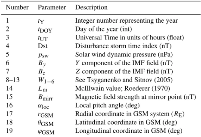
Fig. 1. Validation of neural network with LANL geosynchronous satellite 1990-095 ephemerides. Top: scatter plot ofL∗values from model (target) against neural network results. Green-dashed line indicates a perfect fit and red solid line indicates the least-square fit to the scatter plot. One thousand ephemeris points and solar wind conditions were randomly chosen between 15 October 2001 and 30 June 2005. Middle: histogram plot of overall residuals from scatter plot. Bottom: residual plot as a function ofL∗.
to the magnetopause for which the magnetic flux integral (Eq. 2) is not defined. Such a discontinuity inL∗ requires a separate ANN. Otherwise, the ANN would simply extrapo-lateL∗into regions where it is in reality not defined. There-fore, we created a second neural networkLANLmaxto de-scribe the maximum possible value forL∗under the specified solar wind conditions. The maximumL∗is often referred to as the last closed drift shell. Table 2 lists the input parame-ters necessary for calculatingLmax. SinceLmaxis describing
a global configuration, the neural networkLANLmaxis inde-pendent of specific ephemerides (r, θ, ϕ) but still a function of equatorial pitch angle αeq due to the drift-shell splitting
effect.
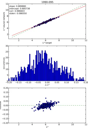
Fig. 2. Validation of neural network with CRRES satellite ephemerides. Top: scatter plot ofL∗values from TS05 model (tar-get) against neural network results. Green-dashed line indicates a perfect fit and red solid line indicates the least-square fit to the scat-ter plot. One thousand ephemeris points and solar wind conditions were randomly chosen between 1 March 1991 and 1 April 1991 and include the geomagnetic superstorm on 24 March 1991 with Dst≈ −300. Middle: histogram plot of overall residuals from scat-ter plot. Bottom: residual plot as a function ofL∗.
to generate the input-output database (see also Koller et al., 2009). We created one million samples with a uniform ran-dom number generator for ephemeris (1.03RE < rGEO<11
RE,−180◦< θ <+180◦,−90◦< ϕ <+90◦) and pitch angle
values (10◦< α
loc<90◦). The solar wind conditions for all
samples are based on randomly selected conditions during a full solar cycle from 1996 to 2007. Solar wind conditions and magnetic field parameters were taken from the Virtual Radiation Belt Observatory (VIRBO, http://virbo.org) based on Qin et al. (2007) using the implementation in SpacePy (Morley et al., 2011).
The second neural networkLANLmaxwas trained with the last closed drift shell calculated withirbem-libas well. We generated 10 000 training examples by using a bisection search algorithm stepping radially outward towards dusk in
Fig. 3. Validation of neural network with GPS-ns41 satellite ephemerides. Top: scatter plot of L∗ values from TS05 model (target) against neural network results. Green-dashed line indicates a perfect fit and red solid line indicates the least-square fit to the scatter plot. One thousand ephemeris points and solar wind con-ditions were randomly chosen between 1–30 April 2004. Middle: histogram plot of overall residuals from scatter plot. Bottom: resid-ual plot as a function ofL∗.
a cartesian solar magnetic (SM) coordinate system. The ac-curacy of the bisection search algorithm for L∗
max was set
to1L∗=0.01. Note, our neural network software only in-cludes a max drift shell modelLANLmaxbut not a separate model for the inner boundary drift loss cone which could be important for low Earth orbiting satellites. However, a standard IGRF model (International Geomagnetic Reference Field) should be sufficient for these altitudes.
We used a constrained truncated Newton algorithm in the ffnetpython module (Wojciechowski, 2009) to train an ANN on the input-target data for both neural networks LANLstarand LANLmax. The training algorithms were specified with a tolerance of 10−6.
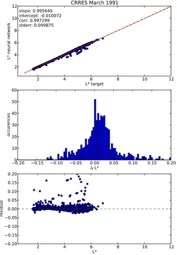
Fig. 4. Validation of neural network with Polar satellite ephemerides. Top: scatter plot ofL∗values from TS05 model (tar-get) against neural network results. Green-dashed line indicates a perfect fit and red solid line indicates the least-square fit to the scat-ter plot. One thousand ephemeris points and solar wind conditions were randomly chosen between 1996–2005 covering a wide range of ephemerides due the precession of the spacecraft. Middle: his-togram plot of overall residuals from scatter plot. Bottom: residual plot as a function ofL∗.
output. In the case that a certain input value is not available, the system will degrade but not necessarily completely fail because the correlation functions are distributed over several other nodes (Reed and Marks, 1999). Our neural network requires the magnetic field strengthBmirrat the mirror point
and the McIlwainLmvalue. For a self-consistent calculation,
one would use the TS05 model to obtain these values. How-ever, one could also use the graceful degradation property of neural networks and calculate these numbers based on a sim-pler magnetic field model or, perhaps, even a dipole field. We will perform a detailed study in a future publication. For this study, however, we have used the self-consistent calculation using TS05 for the validation below.
Using additional, and to some degree redundant, input parameters for a neural network can lead to overfitting.
Fig. 5. Validation of neural network with ephemerides from one of the RBSP satellites using an example ephemeris file of this fu-ture mission and mapping them to solar wind condition between February 2000 and January 2002. Top: scatter plot ofL∗values from TS05 model (target) against neural network results. Green-dashed line indicates a perfect fit and red solid line indicates the least-square fit to the scatter plot. One thousand ephemeris points and solar wind conditions were randomly chosen for the above time period. Middle: histogram plot of overall residuals from scatter plot. Bottom: residual plot as a function ofL∗.
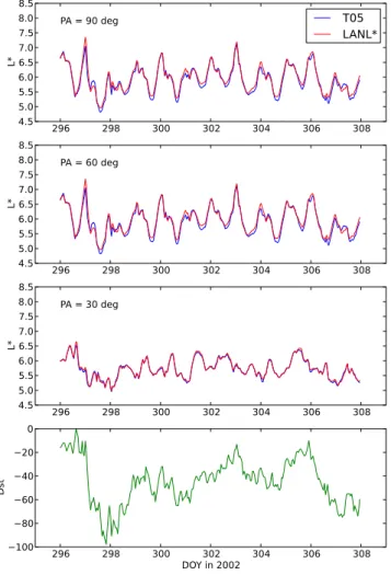
Fig. 6. Calculating the L∗ time series during a moderate storm with Dst =−100 nT following the ephemerides of LANL geosyn-chronous satellite 1990-095. The geomagnetic storm had its Dst minimum close to 25 October 2002 (DOY = 298). TheL∗values from the underlying TS05 model (blue) and from the LANL∗ neu-ral network (red) are compared for 90, 60, 30◦pitch angles. The bottom panel shows the disturbance storm time index (Dst) for this period.
4 Validation study
We validated both neural networks with completely indepen-dent data using a selection of actual satellite ephemerides. These ephemerides and solar wind conditions where not part of the training data set. The first example is shown in Fig. 1 using LANL geosynchronous satellite 1990-095. We ran-domly selected 1000 ephemeris locations between 15 Oc-tober 2001 and 30 June 2005 and calculatedL∗ based on both the TS05 model and LANL∗. They agree quite well with a standard error of1L∗≈0.088 which corresponds to 1.3 %. This accuracy is sufficient for a scientific studies as it is much better than the accuracy of the underlying magnetic field model. However, it does not reflect the accuracy of the integration method.
Fig. 7. Time series plot of the last closed drift shellLmaxas it
was calculated for solar wind conditions from 23 October 2002 to 4 November 2002 using TS05 (blue) and the LANL* neural net-work (red) for pitch angleαloc= 90◦. Even for a moderate storm,
the last closed drift shell can vary betweenL∗= 6−9.5.
Pitch angles for this and all other validation were randomly selected between 10◦< α
loc<90◦.
Another independent validation is shown in Fig. 2. We randomly selected 1000 ephemeris points between 1 March 1991 and 1 April 1991 from the CRRES satellite orbit. Note that this is outside of the solar cycle data used for the training data. This also includes the extreme storm from 24 March 1991 with a Dstmin≈ −300 nT. The neural
network performs very well for this geo-transfer orbit with a standard error of1L∗≈0.1.
We achieved the best result with GPS-ns41 ephemerides (Fig. 3). GSP-ns41 is in a circular orbit with r≈4.2RE.
Again, we selected 1000 random ephemeris locations be-tween 1–30 April 2004. The standard error is1L∗≈0.04, which corresponds to a 1 % error.
The 1000 ephemeris locations for the Polar satellite (Fig. 4) were randomly selected between 1996–2005 cover-ing a wide range of ephemerides due the precession of the spacecraft. The standard error for this polar type orbit is
1L∗≈0.1 for randomly chosen local pitch angles.
Figure 5 shows the validation study for a “virtual” RBSP satellite (Radiation Belt Storm Probes) which is a future NASA mission, planned to launch in May 2012. The fu-ture ephemeris was mapped back in time to start in ary 2000. We selected 1000 random point between Febru-ary 2000 and JanuFebru-ary 2002 for the validation. The standard error is1L∗≈0.06.
We also provide a time series figure for a particular storm on 25 October 2002. This geomagnetic storm com-menced due to a high speed solar wind stream resulting in a Dst =−100 nT. Figure 6 shows a comparison of the neural network LANL∗ versus the TS05 model for three different local pitch anglesαloc= 90◦, 60◦, 30◦. Figure 7 shows a time
5 Conclusion and summary
We have presented a new version of our LANL∗ model to calculateL∗, which is a computationally intensive but im-portant input parameter for radiation belt models. Accurate magnetic field models have been neglected for calculating this value due to the computational burden and often a sim-ple dipole field is used instead. Our model can calculateL∗ based on a sophisticated dynamic magnetic field model at a fraction of the time required for full drift shell integration us-ing a neural network technique. Once all input parameters for the neural network are assembled, one million calcula-tion will only take a few seconds to run on a modern desktop computer. This is a speedup of almost six orders of magni-tudes while adding only a few percent of error to the output which is negligible considering the uncertainty in the under-lying magnetic field model TS05 itself.
This new, computationally efficient model is particularly important for real-time processing of space weather applica-tions and studies involving solar cycles of data sets. While this particular version has only been trained with the TS05 model, the technique itself is applicable to other magnetic field models as well. We are currently working on develop-ing a neural network for a variety of empirical magnetic field models and self-consistent physics based numerical models like RAM-SCB (Zaharia et al., 2006).
The LANL∗neural network model is available for down-load at http://www.lanlstar.net.
Acknowledgements. The authors would like to thank Geof-frey Reeves and Reiner Friedel at Los Alamos National Laboratory for the numerous helpful discussion and also acknowledge the SpacePy project which provided an extremely useful library of space physics functions and codes which is available at http://spacepy.lanl.gov. This work has been supported by the National Science Foundation (grant ATM-0718710) and NASA (grant NNH10AP06I).
Edited by: D. Lunt
References
Boscher, D., Bourdarie, S., O’Brien, P., and Guild, T.: IRBEM-LIB library Rev275, http://irbem.sourceforge.net/ (last access: 21 De-cember 2010), 2010.
Chen, Y., Friedel, R. H. W., and Reeves, G. D.: Phase space den-sity distributions of energetic electrons in the outer radiation belt during two Geospace Environment Modeling Inner Magneto-sphere/Storms selected storms, J. Geophys. Res.h, 111(A11S04), 1–12, doi:10.1029/2006JA011703, 2006.
Huang, C.-L., Spence, H. E., Singer, H. J., and Tsyganenko, N. A.: A quantitative assessment of empirical magnetic field models at geosynchronous orbit during magnetic storms, J.Geophys. Res.-Space, 113, A04208, doi:10.1029/2007JA012623, 2008. Koller, J., Reeves, G. D., and Friedel, R. H. W.: LANL∗V1.0: a
ra-diation belt drift shell model suitable for real-time and reanalysis applications, Geosci. Model Dev., 2, 113–122, doi:10.5194/gmd-2-113-2009, 2009.
McCollough, J. P., Gannon, J. L., Baker, D. N., and Gehmeyr, M.: A statistical comparison of commonly used exter-nal magnetic field models, Space Weather, 6, S10001, doi:10.1029/2008SW000391, 2008.
Morley, S., Koller, J., Welling, D. T., and Henderson, M. G.: SpacePy – A Python-based library of tools for the space sciences, in: SciPy 2010 Proceedings, available at http://spacepy.lanl.gov, (last access: March 2011), in press, 2011.
Olson, W. P. and Pfitzer, K. A.: A Quantitative Model of the Mag-netospheric Magnetic Field, J. Geophys. Res., 79, 3739–3748, doi:10.1029/JA079i025p03739, 1974.
Qin, Z., Denton, R. E., Tsyganenko, N. A., and Wolf, S.: Solar wind parameters for magnetospheric magnetic field modeling, Adv. Space Res., 5, S11003, doi:10.1029/2006SW000296, 2007. Reed, R. D. and Marks, R. J.: Neural smithing : supervised learning in feedforward artificial neural networks, The MIT Press, Cam-bridge, Mass., 1999.
Roederer, J. G.: Dynamics of geomagnetically trapped radiation, in: Physics and chemistry in space, v. 2, Springer-Verlag, Berlin, New York, 1970.
Schulz, M.: The magnetosphere, Geomagnetism, 4, 87–293, 1991. Schulz, M. and Lanzerotti, L. J.: Particle diffusion in the
radia-tion belts, in: Physics and chemistry in space, v. 7, edited by: Schulz, M. and Lanzerotti, L. J., Springer-Verlag, Berlin, New York, 1974.
Tsyganenko, N. A. and Sitnov, M. I.: Modeling the dynamics of the inner magnetosphere during strong geomagnetic storms, J. Geo-phys. Res.-Space, 110, A03208, doi:10.1029/2004JA010798, 2005.
Tsyganenko, N. A and Sitnov, M. I.: Magnetospheric configura-tions from a high-resolution data-based magnetic field model, J. Geophys. Res., 112, A06225, doi:10.1029/2007JA012260, 2007. Tsyganenko, N. A., Singer, H. J., and Kasper, J. C.: Storm-time distortion of the inner magnetosphere: How severe can it get?, J. Geophys. Res.-Space, 108, SMP 18-1, CiteID 1209, doi:10.1029/2002JA009808, 2003.
Wojciechowski, M.: ffnet: Feed-forward neural network for python, http://ffnet.sourceforge.net/, (last access: 12 November 2009), Version 0.6.2, 2009.
Wolf, R.: Magnetospheric Configuration, in: Introductin to Space Physics, edited by Kivelson, M. G. and Russell, C. T., Cam-bridge, Chapt. 10, 288–325, 1996.