Transfer function models to quantify the delay between air and ground temperatures in thawed active layers

(1)

TCD

5, 2935–2966, 2011

Quantifying the delay between air and ground temperatures

E. Zenklusen Mutter et al.

Title Page

Abstract Introduction

Conclusions References

Tables Figures

◭ ◮

Back Close

Full Screen / Esc

Printer-friendly Version Interactive Discussion

Discussion

P

a

per

|

Dis

cussion

P

a

per

|

Discussion

P

a

per

|

Discussio

n

P

a

per

The Cryosphere Discuss., 5, 2935–2966, 2011 www.the-cryosphere-discuss.net/5/2935/2011/ doi:10.5194/tcd-5-2935-2011

The Cryosphere Discussions

This discussion paper is/has been under review for the journal The Cryosphere (TC). Please refer to the corresponding final paper in TC if available.

Transfer function models to quantify the

delay between air and ground

temperatures in thawed active layers

E. Zenklusen Mutter1, J. Blanchet2, and M. Phillips1

1

WSL Institute for Snow and Avalanche Research SLF, Fl ¨uelastrasse 11, 7260 Davos Dorf, Switzerland

2_´

Ecole Polytechnique F ´ed ´erale de Lausanne EPFL, 1015 Lausanne, Switzerland

Received: 6 October 2011 – Accepted: 12 October 2011 – Published: 26 October 2011

Correspondence to: E. Zenklusen Mutter (zenklusen@slf.ch)

(2)

TCD

5, 2935–2966, 2011

Title Page

Tables Figures

◭ ◮

Back Close

Full Screen / Esc

Discussion

P

a

per

|

Dis

cussion

P

a

per

|

Discussion

P

a

per

|

Discussio

n

P

a

per

|

Abstract

Air temperatures influence ground temperatures with a certain delay, which increases with depth. Borehole temperatures measured at 0.5 m depth in Alpine permafrost and air temperatures measured at or near the boreholes have been used to model this dependency. Statistical transfer function models have been fitted to the daily di_fference

5

series of air and ground temperatures measured at seven different permafrost sites in the Swiss Alps.

The relation between air and ground temperature is influenced by various factors such as ground surface cover, snow depth, water or ground ice content. To avoid complications induced by the insulating properties of the snow cover and by phase

10

changes in the ground, only the mostly snow-free summer period when the ground at 0.5 m depth is thawed has been considered here. All summers from 2006 to 2009 have been analysed, with the main focus on summer 2006.

The results reveal that in summer 2006 daily air temperature changes influence ground temperatures at 0.5 m depth with a delay ranging from one to six days,

depend-15

ing on the site. The fastest response times are found for a very coarse grained, blocky rock glacier site whereas slower response times are found for blocky scree slopes with smaller grain sizes.

1 Introduction

Ground temperature depends on air temperature, ground surface characteristics (e.g.

20

the presence of vegetation or scree), snow cover and ground properties such as grain size and water/ice content (Goodrich, 1982; Harris and Pedersen, 1998; Gorbunov et al., 2004; Luetschg et al., 2004; Zhang, 2005; Gruber and Hoelzle, 2008).

Air temperature changes will sooner or later induce changes in the thermal state of the ground. The active layer is the uppermost part of permafrost, and is subject to

sea-25

(3)

TCD

5, 2935–2966, 2011

Title Page

Tables Figures

◭ ◮

Back Close

Full Screen / Esc

Discussion

P

a

per

|

Dis

cussion

P

a

per

|

Discussion

P

a

per

|

Discussio

n

P

a

per

and therefore reacts first to changing weather and climate. Increasing air temperatures can lead to active layer deepening and ground instabilities, which can cause problems for infrastructure (Phillips and Margreth, 2008; Bommer et al., 2010) and in mountain-ous terrain lead to mass movements like rock falls or debris flows (Noetzli et al., 2003; Gruber et al., 2004b; Rabatel et al., 2008; Harris et al., 2009). It is therefore of interest

5

to know how permafrost reacts to changing environmental conditions and in particular to changes in air temperature.

Various approaches have been applied to investigate the relation between air and ground temperature (e.g. Geiger, 1965; Harlan and Nixon, 1978; Beltrami, 1996; Frauenfeld et al., 2004; Smerdon et al., 2004, 2009). For example Harlan and

10

Nixon (1978) described the influence of the accumulated thawing temperatures, soil properties and moisture content on the active layer thickness. This approach was later applied in different studies, in both high latitude and high altitude permafrost re-gions (e.g. Brown et al., 2000; Hinkel and Nelson, 2003; Christiansen, 2004; Mazhitova et al., 2004; ˚Akerman and Johansson, 2008; Smith et al., 2009; Zenklusen Mutter and

15

Phillips, 2011).

In the Alps the heterogeneity of the surface and subsurface, as well as the com-plex topography complicate the modelling of ground temperature (Gruber et al., 2004a; Noetzli et al., 2007). It is for example still a big challenge to model precipitation in mountainous terrain and hence estimate its influence on permafrost (Frei et al., 2003;

20

Salzmann et al., 2007). Furthermore, there are still too few borehole sites in the Alps for a complete overview of the complex thermal conditions reigning in the ground. In order to analyze the future evolution of the thermal state and ground ice content in permafrost, empirical, analytical and numerical physically-based model approaches of different complexity are usually taken (Riseborough et al., 2008; Harris et al., 2009;

25

(4)

TCD

5, 2935–2966, 2011

Title Page

Tables Figures

◭ ◮

Back Close

Full Screen / Esc

Discussion

P

a

per

|

Dis

cussion

P

a

per

|

Discussion

P

a

per

|

Discussio

n

P

a

per

|

Swiss Alps, summer temperature changes during the snow-free period and the timing of the first snow cover in autumn have the largest impact on ground temperatures.

Unlike these physically-based approaches, this study presents a statistical model to identify the temporal relation between day-to-day changes in the air temperature and those in the ground temperature of Alpine permafrost soils. Using a transfer function

5

model, ground temperature changes measured in permafrost boreholes are linked to corresponding changes in air temperature. The goal is to quantify the temporal de-pendence of ground temperature changes on air temperature changes and find out whether this dependence is similar for all the different sites or if site-specific properties such as lithology, hydrology or ground-ice content alter the relation, and if so, to what

10

extent. As the snow cover and thawing/freezing processes decouple ground tempera-tures from air temperatempera-tures (Luetschg et al., 2004; Zhang, 2005), only a three-month period in summer 2006 during which the active layer was established is here consid-ered in detail. Ground temperatures measured in boreholes at 0.5 m depth in the active layer and air temperatures measured at or near the borehole sites are modelled

sta-15

tistically. Furthermore, all summers from 2006 to 2009 have been analysed in order to place the 2006 results in a larger context.

2 Data

Daily ground temperatures used for this work were measured in seven boreholes lo-cated in mountain permafrost at elevations between 2400 m a.s.l. and 3295 m a.s.l. in

20

the Swiss Alps (Fig. 1 and Table 1).

Yellow Springs Instruments thermistors (YSI 44008) are used for the borehole tem-perature measurements, in combination with Campbell CR10X or CR1000 data log-gers, with a calibrated precision of 0.01–0.02◦_C.

The borehole sites are located in different types of terrain (Table 1 and Fig. 11),

in-25

(5)

TCD

5, 2935–2966, 2011

Title Page

Tables Figures

◭ ◮

Back Close

Full Screen / Esc

Discussion

P

a

per

|

Dis

cussion

P

a

per

|

Discussion

P

a

per

|

Discussio

n

P

a

per

are of different lengths and the depth of the boreholes at the study sites varies from about 20 m to more than 50 m. For the analyses carried out in this study mean daily ground temperatures in the active layer (at 0.5 m depth) and mean daily air tempera-tures either from a meteorological station at the borehole site or nearby (IMIS network, WSL Institute for Snow and Avalanche Research SLF) have been used (see Fig. 1

5

and Table 2). An overview of the mean daily air and ground temperature time series for summer 2006 (1 July to 30 September) measured at the different sites is given in Figs. 2 and 3.

3 Statistical methods and results

Statistical transfer function models have been applied to model the influence of air

10

temperature on ground temperature. In the following, the procedure will be presented with example data from site A2 and summer 2006. The general framework follows the procedure of chapter 11.4 of Cryer and Chan (2010); see also Chapt. 11 in Box et al. (2008), Chapt. 5.7 in Shumway and Sto_ffer (2011).

As there is no weather station close to borehole A2, air temperatures have been

15

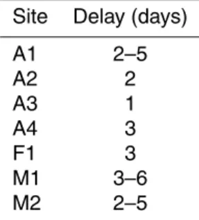
taken from the station Met.Ab which is located 9.2 km away at a comparable elevation (Tables 1 and 2). The courses of air and ground temperature show clear similarities (Fig. 3). However, there is a period of 23 days in the middle of the summer where discrepancies are visible. These are due to the presence of snow which attenuates the relation between both parameters. However, for simplicity these discrepancies have

20

not been taken into consideration.

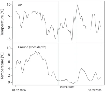
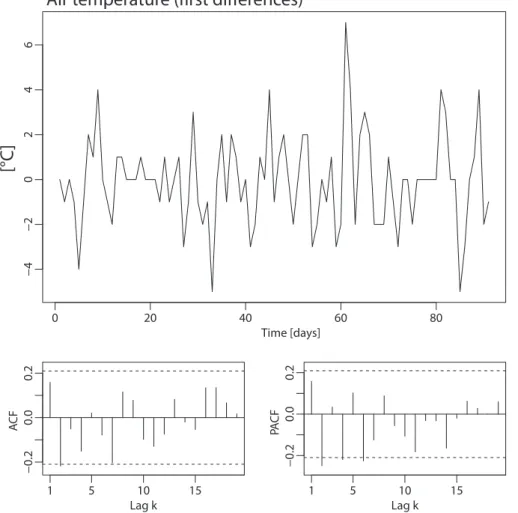
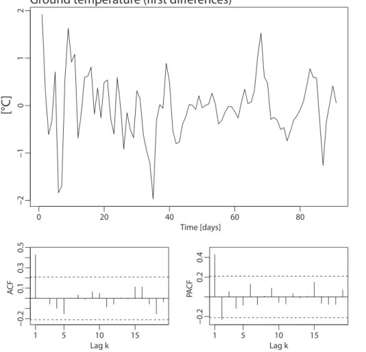
To determine the influence of air temperature on ground temperature, transfer func-tions were used to model the first di_fferences of both temperature series (Figs. 4 and 5, top graphs). The idea behind this is to explain to which extent and with what delay, for example, a 10◦C change in air temperature from one day to another is represented

25

(6)

TCD

5, 2935–2966, 2011

Title Page

Tables Figures

◭ ◮

Back Close

Full Screen / Esc

Discussion

P

a

per

|

Dis

cussion

P

a

per

|

Discussion

P

a

per

|

Discussio

n

P

a

per

|

the Kwiatkowski-Phillips-Schmidt-Shin (KPSS) test (Kwiatkowski et al., 1992) reveals that the air and ground temperature di_fference series from site A2 can be assumed to be stationary. They are however autocorrelated (Fig. 4 and Fig. 5, bottom graphs) and mutually dependent, as are the initial ground and air temperature series them-selves. Our goal is to quantify how changes in ground temperature are influenced by

5

present and past changes in air temperature. According to Cryer and Chan (2010), the following general regression model relating the two time series can be considered:

Y_t₌ ∞

X

k=−∞

β_kX_t−_k₊Z_t. (1)

In Eq. (1) parameterX_t describes the input data (i.e. in our case the air temperature difference series), Y_t the output data (i.e. in our case ground temperature difference

10

series) andZ_t corresponds to an error term, assumed to be independent of X_t. Index

t labels the time (i.e. days here) ranging from 1 to n. Parameter β_k labels an infinite number of regression coefficients describing the dependency of the output on the input time series. In real applications however, a finite sum of coe_fficients is used and the model simplifies to

15

Y_t₌

m₂

X

k=m₁

β_kX_t−_k₊Z_t t₌m₂₊1,...,n . (2)

Equation (2) is just a linear model for the ground temperature differences with the lagged air temperature di_fferences as a covariate. It is known variously as the transfer function model, the finite distributed lag model, or the dynamic regression model. In our case, the input seriesX_t(air temperature changes) influences the outputY_t(ground

20

(7)

TCD

5, 2935–2966, 2011

Title Page

Tables Figures

◭ ◮

Back Close

Full Screen / Esc

Discussion

P

a

per

|

Dis

cussion

P

a

per

|

Discussion

P

a

per

|

Discussio

n

P

a

per

efficiently and quickly to air temperature, and moderately large β_k up to a quite large lag (e.g.k₌5 or 6) in ground that has a di_ffuse response to air temperature. These coe_fficientsβ_k need to be estimated from the data. There are two possibilities for this. The first is to assume some structure on the relation of the coefficientsβ_k. The most important structure is the Almon lag model (Almon, 1965), see chapter 15 of Judge

5

et al. (1985) for a review. The second possibility is to impose no structure on theβ_k

and let the data decide the shape of the lag structure. This is the approach we follow here. In Eq. (2), the coe_fficients β_k are thus (m₂−m₁₊1) unstructured regression coe_fficients to be estimated.

Equation (2) can be written in vector form as

10

Y ₌Xβ₊Z, (3)

whereY is the (n₋m₂)_×1 vector [Y_m

2+1,...,Yn],Xis the (n−m2)×(m2−m1+1) matrix

of lagged output values, whosei-th row is composed of elements [X_m

2−m1+i,...,Xi],βis

the (m₂₋m₁₊1)×1 vector [βm₁,...,βm₂], andZis the (n−m2)×1 vector [Zm₂+1,...,Zn].

As the inputX_t and the output Y_t are stationary autocorrelated (Figs. 4 and 5 for the

15

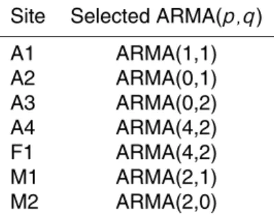
example site A2), the same is expected for the error termZ_t. Hence, we assumed in the regression model Eq. (2) thatZ_t follows some ARMA(p,q). Given arbitrary values for

m₁,m₂,pandq, standard methods for dealing with correlated errors in linear models can be used to fit the transfer model Eq. (2). However, in practicem₁,m₂,pandq are unknown and reasonable values have to be chosen before being able to estimate the

20

model.

We chose m₁ and m₂ according to the procedure described in Cryer and Chan (2010). The selection is made on a transformed version of model Eq. (2), obtained as follows. The stationary autocorrelated X_t are assumed to follow some ARMA(p′,q′) model. The seriesX_t being observed, we can use standard techniques

25

(8)

TCD

5, 2935–2966, 2011

Title Page

Tables Figures

◭ ◮

Back Close

Full Screen / Esc

Discussion

P

a

per

|

Dis

cussion

P

a

per

|

Discussion

P

a

per

|

Discussio

n

P

a

per

|

˜

X_t₌1−π1B−π2B2−...

X_t₌π(B)X_t, (4)

is then a white noise series. Applying the filterπ(B) to both sides of Eq. (2) now gives

˜

Y_t₌

m₂

X

k=m₁

β_kX˜_t−_k₊Z˜_t, (5)

where

˜

X_t ₌X_t₋π₁X_t₋₁₋π₂X_t₋₂_{− ···},

5

˜

Y_t ₌Y_t₋π₁Y_t−1₋π₂Y_t−2_{− ···},

˜

Z_t ₌Z_t₋π₁Z_t−1₋π₂Z_t−2_{− ···}.

BecauseX˜ is a white noise andX˜ is independent ofZ˜, the theoretical cross-correlation between the transformed processes X˜ and Y˜ at lag k, Corr( ˜X_t−_k,Y˜_t), is then propor-tional to the regression coe_fficient β_k. Thus in the cross-correlation plot (CCF plot)

10

of ˜X_t and ˜Y_t CCF values should be almost 0 for k < m₁ and k > m₂, or at least non-significant. Therefore, the CCF plot between ˜X_tand ˜Y_t can be used as a graphical tool for the selection ofm₁andm₂.

In Fig. 6 the CCF-Plot for site A2 is depicted, revealingm₁₌0 andm₂₌4 as possible candidates. However, when applied to the data of all seven sites, lags ranging from

15

m₂₌1 (site A3) to m₂₌6 (site M2) are revealed (not shown). Considering di_fferent values ofm₁andm₂for the different boreholes would impede intra-site comparisons of the estimated regression coe_fficients, and thus would make the intra-site comparison of the reaction speed of ground temperature changes to air temperature changes di_fficult. Another possibility therefore is to assume a fixed number of lags m₁ and m₂ in the

20

regression model Eq. (2) for all sites and to distinguish the significant coefficientsβ_k

(9)

TCD

5, 2935–2966, 2011

Title Page

Tables Figures

◭ ◮

Back Close

Full Screen / Esc

Discussion

P

a

per

|

Dis

cussion

P

a

per

|

Discussion

P

a

per

|

Discussio

n

P

a

per

Oncem₁andm₂have been selected, the choice of the orderspandqfor the ARMA model for the residuals Z_t in Eq. (2) remains. The di_fficulty arises because Z_t is not observed. A first possibility would be to choose appropriate orders p and q based on the residuals obtained by fitting model Eq. (2) under the improper assumption of uncorrelated residuals, and then to use these orders to properly fit model Eq. (2).

5

However, we preferred at this point to have a more automatic criterion in order to be able to apply the procedure automatically to all our boreholes. The choice we made was to fit di_fferent models Eq. (2) withm₁₌0 andm₂₌8 and for di_fferent orderspand

q, chosen to be relatively small to restrict the number of free parameters. We allowedp

ranging from 0 to 8 andqranging from 0 to 2. This leads to 27 different models Eq. (2)

10

with 9 to 19 free parameters. All these models were fitted using the R function arima, with argument “xreg” set to the appropriate matrixXof Eq. (3). It uses the well-known Cochrane-Orcutt procedure (Cochrane and Orcutt, 1949) for fitting linear models with correlated errors. Finally the model with the lowest AIC value was selected as the best one (Akaike, 1973).

15

In summary, the applied procedure for fitting the transfer function model to the diff er-ence seriesX_tandY_t can be described as follows:

1. Find an appropriate ARMA(p′,q′) for theX_t. Prewhiten the input dataX_t with the corresponding filter, leading to ˜X_t(Eq. 4).

2. Transform the output dataY_t by applying the same filter as in step 1 (Eq. 5). Call

20

the transformed output data ˜Y_t.

3. Create a cross-correlation plot between ˜X_t and ˜Y_t. Deduce from it candidates for

m₁andm₂.

4. Fit model Eq. (2) for this choice ofm₁andm₂, with di_fferent orderspandqfor the ARMA(p,q) model of the residualsZ_t. Choose the one which best fits the data

25

(10)

TCD

5, 2935–2966, 2011

Title Page

Tables Figures

◭ ◮

Back Close

Full Screen / Esc

Discussion

P

a

per

|

Dis

cussion

P

a

per

|

Discussion

P

a

per

|

Discussio

n

P

a

per

|

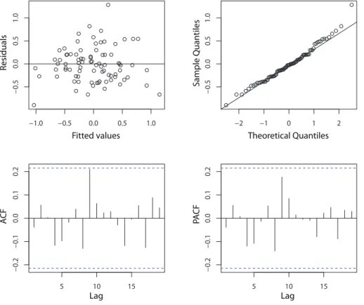
For the example site A2 an ARMA(0,1) (i.e. an MA(1)) model has been selected for the residualsZ_t (Table 3). In total this selected model Eq. (2) has 10 parameters. The residual analysis plots show that the residuals in the MA(1) model for Z_t are uncor-related and normally distributed (Fig. 7). The application of the Ljung-Box test (Ljung and Box, 1978) for site A2 and di_fferent lags ranging from 1 to 15 reveals P values

5

from 0.5 (lag 9) to almost 1 (lag 3) and confirms that the residuals are “white noise”. This is consistent with the theory of the transfer model. The comparison of the fitted with the measured di_fference data also shows a relatively good fit of the transfer model (Fig. 8, upper graph). However, positive di_fferences seem to be slightly underestimated whereas negative differences are rather overestimated, leading to a little less

fluctua-10

tion than observed.

Although model Eq. (2) applies to the di_fference data and not to the air and ground temperatures directly, one can now use these fitted values to reconstruct the time series of ground temperatures at dayt₊1, given the ground temperature at dayt. LetY′

t be

the observed ground temperature at dayt. Hence, the predicted value ˆY_t′₊₁ can now

15

be obtained fortranging fromm₂₊1 ton₋1 from the valueY_t′ and the predicted first difference ˆY_tof Eq. (2) by

ˆ

Y′

t+1=Yt′+Yˆt, for t=m2+1,...,n−1. (6)

This so-called “one-day ahead prediction” can be used for example if there is a miss-ing value at day t₊1 in the ground temperature series, but the air temperature is

20

available. The comparison of these one-day ahead predicted and measured ground temperatures confirms the good fit of the transfer function model (Fig. 8, lower graph). The estimated regression coefficients β_k of model Eq. (2) for summer 2006 in A2 are shown in Fig. 9, dotted in black. They reach their maximum at lagk₌2, meaning that air temperature changes occur at 0.5 m depth with a delay of around two days

25

(11)

TCD

5, 2935–2966, 2011

Title Page

Tables Figures

◭ ◮

Back Close

Full Screen / Esc

Discussion

P

a

per

|

Dis

cussion

P

a

per

|

Discussion

P

a

per

|

Discussio

n

P

a

per

from the other six borehole sites. The estimated regression coefficientsβ_k are plotted in Fig. 10. Comparing these coe_fficients for all sites reveals that depending on the site, the delay between air temperature changes and ground temperature changes at 0.5 m depth varies from about one to six days in summer 2006 (Figs. 9, 10 and Table 4). These di_fferences can be explained by the di_fferent ground properties at the borehole

5

sites.

The fastest response occurs at site A3, with a delay of one day (Table 4). The bore-hole also shows much higher values of the regression coe_fficients β_k than the other sites (Figs. 9 and 10). This fast and e_fficient response can be explained by the very coarse, blocky surface cover at A3 (Fig. 11c) which allows an efficient relation between

10

air and ground temperature changes. For site A2, which is located on a weather-exposed ridge (Fig. 11b), the delay is around two days (Fig. 9). On the contrary, scree slope sites A1, F1, M1 and M2 show more delayed and prolonged response times (Fig. 10, Table 4). The surface at these sites is not as coarse-grained as at site A3 (Fig. 11a,c,e,f) and the scree still contains air-filled voids, providing good thermal

15

insulation. Although sites M1 and M2 are located only 50 m away from each other, differences in snow cover distribution (M1 lies between avalanche defence structures, which cause delayed snow melt, see also Fig. 11f) and hydrology (Rist and Phillips, 2005) lead to a slightly longer response time at M1 than at M2 (Table 4). Finally, in the artificially modified finer-grained terrain site A4, located at a chairlift midway station

20

(Fig. 11d), similar responses as for the scree slopes are found, although less di_ffuse (Fig. 10c).

In addition to summer 2006, we applied the same procedure to data acquired in sum-mers 2007, 2008 and 2009. The grey area in Figs. 9 and 10 depicts the enveloping curves of the estimated regression coefficients for these four summers. The overall

25

(12)

TCD

5, 2935–2966, 2011

Title Page

Tables Figures

◭ ◮

Back Close

Full Screen / Esc

Discussion

P

a

per

|

Dis

cussion

P

a

per

|

Discussion

P

a

per

|

Discussio

n

P

a

per

|

(see also Fig. 3) and a weak relation between air and ground temperature results in small regression coe_fficientsβ_k. The presence of snow in summer 2008 in A2 was due to the presence of a huge snow cornice from the previous winter (K. Lauber, personal communication, 2008), causing the low model coefficients at the lower border of the grey area in Fig. 9. On the other hand, sites A3, A4 and F1 show very low

variabil-5

ity over the four summers. At site A4 the borehole is located at the chairlift station where the regular artificial maintenance of the snow cover impedes the establishment of seasonally varying snow depths at the end of the winter. Seasonal di_fferences at A4 are therefore restrained to summer snow events which have no long temporal implica-tions. At A3 and F1 the narrowness of the envelope is probably simply due to similar

10

conditions for the summers of the period 2006 to 2009.

4 Discussion and outlook

Transfer function models have been fitted to air and ground temperature data measured at 0.5 m depth at seven di_fferent permafrost sites in the Swiss Alps. Due to the influence of snow cover and ground ice on the relation between ground temperature and air

15

temperature, the model has only been fitted for the mostly snow-free summer period when the ground at 0.5 m depth is thawed.

Estimated model coefficients show that the ground temperature changes at 0.5 m depth at different permafrost sites depend on the air temperature changes which oc-curred about one to six days earlier, depending on the site characteristics. Very

coarse-20

grained, blocky ground surfaces lead to faster response times. Smaller-scale blocks in scree slopes insulate the ground below and therefore induce longer response times. For some sites the relation between air and ground temperature – and therefore the co-e_fficient estimates – were influenced by short periods with summer snow cover, which was not taken into account for this study. The study confirms the well-known influence

25

(13)

TCD

5, 2935–2966, 2011

Title Page

Tables Figures

◭ ◮

Back Close

Full Screen / Esc

Discussion

P

a

per

|

Dis

cussion

P

a

per

|

Discussion

P

a

per

|

Discussio

n

P

a

per

A subdivision of the year into snow-free and snow-covered, frozen and thawed time periods could be helpful to determine the role of various disturbing factors and is planned in future. Furthermore, the derivation of physical parameters such as heat capacity, thermal conductivity and hence thermal diffusivity from the model coefficients might be an interesting and important step to follow. Other questions of interest in this

5

context are, for example, to estimate to what depth ground temperatures are influenced by daily or seasonal air temperature changes, or to determine the optimal vertical ther-mistor distribution and temporal resolution for borehole temperature measurements.

Acknowledgements. The idea for this study originates from a diploma thesis developed by the main author for the course “Weiterbildungslehrgang in Angewandter Statistik” at ETH 10

Zurich. However, the methods and results presented here differ from those applied in that

earlier work and were carried out in the context of the CCES-EXTREMES project (http: //www.cces.ethz.ch/projects/hazri/EXTREMES). Special thanks are addressed to M. Dettling, A. Davison and M. Lehning for their valuable contributions. Funding for the site investigations was provided by the Swiss cantons Grisons and Valais and logistic support was given by the 15

Bergbahnen Gr ¨achen. The members of the SLF electronics team are sincerely thanked for their technical support. Five of the seven boreholes are in PERMOS, the Swiss permafrost monitoring network.

References

Akaike, H.: A new look at the statistical model identification, IEEE T. Autom. Contr., 19, 716– 20

723, 1973. ˚

Akerman, H. J. and Johansson, M.: Thawing permafrost and thicker active layers in Sub-arctic Sweden, Permafrost Periglac., 19, 279–292, doi:10.1002/ppp.626, 2008.

Almon, S.: The distributed lag between capital appropriations and expenditures, Econometrica, 33, 178–196, 1965.

25

Beltrami, H.: Active layer distortion of annual air/soil thermal orbits, Permafrost Periglac., 7, 101–110, 1996.

(14)

TCD

5, 2935–2966, 2011

Title Page

Tables Figures

◭ ◮

Back Close

Full Screen / Esc

Discussion

P

a

per

|

Dis

cussion

P

a

per

|

Discussion

P

a

per

|

Discussio

n

P

a

per

|

for planning, constructing and maintaining infrastructure in mountain permafrost, Permafrost Periglac., 21, 97–104, doi:10.1002/ppp.679, 2010.

Box, G. E. P., Jenkins, G. M., and Reinsel, G. C.: Time Series Analysis, Forecasting and Control, Wiley & Sons, Inc., Hoboken, New Jersey, 746 pp., 2008.

Brown, J., Hinkel, K. M., and Nelson, F. E.: The circumpolar active layer

monitor-5

ing (calm) program: research designs and initial results, Polar Geogr., 24, 166–258, doi:10.1080/10889370009377698, 2000.

Burn, C. R.: Short communication: the active layer: two contrasting definitions, Permafrost Periglac., 9, 411–416, 1998.

Christiansen, H. H.: Meteorological control on interannual spatial and temporal variations in 10

snow cover and ground thawing in two Northeast Greenlandic Circumpolar-Active-Layer-Monitoring (CALM) sites, Permafrost Periglac., 15, 155–169, doi:10.1002/ppp.489, 2004. Cochrane, D. and Orcutt, G. H.: Applications of least squares regression to relationships

con-taining autocorrelated errors, J. Am. Stat. Assoc., 44, 32–61, 1949.

Cryer, J. D. and Chan, K.-S.: Time Series Analysis – with Applications in R, Springer Science 15

and Business Media, LLC United States of America, New York, 491 pp., 2010.

Dall’Amico, M., Endrizzi, S., Gruber, S., and Rigon, R.: A robust and energy-conserving model of freezing variably-saturated soil, The Cryosphere, 5, 469–484, doi:10.5194/tc-5-469-2011, 2011.

Engelhardt, M., Hauck, C., and Salzmann, N.: Influence of atmospheric forcing parameters on 20

modelled mountain permafrost evolution, Meteorol. Z., 19(5), 491–500, doi:10.1127/0941-2948/2010/0476, 2010.

Frauenfeld, O. W., Zhang, T., and Barry, R. G.: Interdecadal changes in seasonal freeze and thaw depths in Russia, J. Geophys. Res., 109, D05101, doi:10.1029/2003JD004245, 2004. Frei, C., Christensen, J. H., D ´equ ´e, M., Jacob, D., Jones, R. G., and Vidale P. L.: Daily pre-25

cipitation statistics in regional climate models: evaluation and intercomparison for European Alps, J. Geophys. Res., 108(D3), 4124, doi:10.1029/2002JD002287, 2003.

Geiger, R.: The Climate Near the Ground, Harvard University Press, Cambridge, MA, 611 pp., 1965.

Goodrich, L. E.: The influence of snow cover on the ground thermal regime, Can. Geotech. J., 30

19, 421–432, 1982.

(15)

TCD

5, 2935–2966, 2011

Title Page

Tables Figures

◭ ◮

Back Close

Full Screen / Esc

Discussion

P

a

per

|

Dis

cussion

P

a

per

|

Discussion

P

a

per

|

Discussio

n

P

a

per

95–98, doi:10.1002/ppp.478, 2004.

Gruber, S. and Hoelzle, M.: The cooling effect of coarse blocks revisited: a modelling study of

a purely conductive mechanism, in: Proc. 9th Int. Conf. Permafrost, Fairbanks, Alaska, 28 June–3 July 2008, vol. 1, 557–561, 2008.

Gruber, S., Hoelzle, M., and Haeberli, W.: Rock-wall temperatures in the Alps: modeling 5

their topographic distribution and regional differences, Permafrost Periglac., 15, 299–307,

doi:10.1002/ppp.501, 2004a.

Gruber, S., Hoelzle, M., and Haeberli, W.: Permafrost thaw and destabilization of

Alpine rock walls in the hot summer of 2003. Geophys. Res. Lett., 31, L13504, doi:10.1029/2004GL020051, 2004b.

10

Harlan, R. L. and Nixon, J. F.: Ground thermal regime, in: Geotechnical Engineering for Cold Regions, MacGraw-Hill, New York, 103–163, 1978.

Harris, C., Arenson, L. U., Christiansen, H. H., Etzelm üller, B., Frauenfelder, R., Gruber, S., Haeberli, W., Hauck, C., Hoelzle, M., Humlum, O., Isaksen, K., K ä äb, A., Kern-L ütschg, M. A., Lehning, M., Matsuoka, N., Murton, J. B., N ötzli, J., Phillips, M., Ross, N., Sep äp äl ä, M., 15

Springman, S. M., and Vonder M ¨uhll, D.: Permafrost and climate in Europe: monitoring and modeling thermal, geomorphological and geotechnical responses, Earth Sci. Rev., 92, 117– 171, doi:10.1016/j.earscirev.2008.12.002, 2009.

Harris, S. A. and Pedersen, D. E.: Thermal regimes beneath coarse blocky materials, Per-mafrost Periglac., 9, 107–120, 1998.

20

Hinkel, K. M. and Nelson, F. E.: Spatial and temporal patterns of active layer thickness at Cir-cumpolar Active Layer Monitoring (CALM) sites in Northern Alaska, 1995–2000, J. Geophys. Res., 108(D2), 8168, doi:10.1029/2001JD000927, 2003.

Judge, G. G., Griffiths, W. E., Carter Hill, R., L ¨utkepohl, H., and Lee, T.-C.: The Theory and

Practice of Econometrics, 2nd edn., John Wiley and Sons, New York, 1019 pp., 1985. 25

Kwiatkowski, D., Phillips, P. C. B., Schmidt, P., and Shin Y.: Testing the null hypothesis of stationarity against the alternative of a unit root, J. Econometrics, 54, 159–178, 1992. Ljung, G. M. and Box G. E. P.: On a measure of lack of fit in time series models, Biometrika,

65, 553–564, 1978.

Luetschg, M., Stoeckli, V., Lehning, M., Haeberli, W., and Ammann W.: Temperatures in two 30

boreholes at Fl ¨uela Pass, Eastern Swiss Alps: the effect of snow redistribution on

(16)

TCD

5, 2935–2966, 2011

Title Page

Tables Figures

◭ ◮

Back Close

Full Screen / Esc

Discussion

P

a

per

|

Dis

cussion

P

a

per

|

Discussion

P

a

per

|

Discussio

n

P

a

per

|

Mazhitova, G., Malkova (Ananjeva), G., Chestnykh, O., and Zamolodchikov, D.: Active-layer spatial and temporal variability at european russian Circumpolar-Active-Layer-Monitoring (CALM) sites, Permafrost Periglac., 15, 123–139, doi:10.1002/ppp.484, 2004.

Noetzli, J., Hoelzle, M., and Haeberli, W.: Mountain permafrost and recent Alpine rockfall events: a GIS-based approach to determine critical factors, in: Proc. 8th Int. Conf. Per-5

mafrost, Zurich, Switzerland, 21–25 July 2003, vol. 2, 827–832, 2003.

Noetzli, J., Gruber, S., Kohl, T., Salzmann, N., and Haeberli, W.: Three-dimensional distribution and evolution of permafrost temperatures in idealized high-mountain topography, J. Geophys. Res., 112, F02S13, doi:10.1029/2006JF000545, 2007.

Phillips, M. and Margreth, S.: Effects of ground temperature and slope deformation on the

10

service life of snow-supporting structures in mountain permafrost: Wisse Schijen, Randa, Swiss Alps, in: Proc. 9th Int. Conf. Permafrost, Fairbanks, Alaska, 28 June–3 July 2008, vol. 2, 1417–1422, 2008.

Phillips, P. C. B. and Perron, P.: Testing for a unit root in time series regression, Biometrika, 75, 335–346, 1988.

15

Rabatel, A., Deline, P., Jaillet, S., and Ravanel, L.: Rock falls in high-alpine rock walls quantified by terrestrial lidar measurements: a case study in the Mont Blanc area, Geophys. Res. Lett., 35, L10502, doi:10.1029/2008GL033424, 2008.

Riseborough, D., Shiklomanov, N., Etzelm ¨uller, B., Gruber, S., and Marchenko, S.: Recent advances in permafrost modelling, Permafrost Periglac., 19, 137–156, doi:10.1002/ppp.615, 20

2008.

Rist, A. and Phillips, M.: First results of investigations on hydrothermal processes within the active layer above alpine permafrost in steep terrain, Norsk Geogr. Tidsskr., 59, 177–183, doi:10.1080/00291950510020574, 2005.

Salzmann, N., Frei, C., Vidale, P. L., and Hoelzle, M.: The application of regional climate model 25

output for the simulation of high-mountain permafrost scenarios, Global Planet. Change, 56, 188–202, doi:10.1016/j.gloplacha.2006.07.006, 2007.

Shumway, R. H. and Stoffer, D. S.: Time Series Analysis and Its Applications – with R Examples,

3rd edn., Springer Science and Business Media, LLC United States of America, New York, 596 pp., 2011.

30

(17)

TCD

5, 2935–2966, 2011

Title Page

Tables Figures

◭ ◮

Back Close

Full Screen / Esc

Discussion

P

a

per

|

Dis

cussion

P

a

per

|

Discussion

P

a

per

|

Discussio

n

P

a

per

Smerdon, J. E., Beltrami, H., Creelman, C., and Bruce Stevens, M.: Characterizing land surface processes: a quantitative analysis using air-ground thermal orbits, J. Geophys. Res., 114, D15102, doi:10.1029/2009JD011768, 2009.

Smith, S. L., Wolfe, S. A., Riseborough, D. W., and Nixon F. M.: Active-layer characteristics and summer climatic indices, Mackenzie Valley, Northwest Territories, Canada, Permafrost 5

Periglac., 20, 201–220, doi:10.1002/ppp.651, 2009.

Zenklusen Mutter, E. and Phillips, M.: Active layer development in ten boreholes in Alpine permafrost terrain, Permafrost Periglac., in review, 2011.

Zhang, T.: Influence of the seasonal snow cover on the ground thermal regime: an overview, Rev. Geophys., 43, RG4002, doi:10.1029/2004RG000157, 2005.

(18)

TCD

5, 2935–2966, 2011

Title Page

Tables Figures

◭ ◮

Back Close

Full Screen / Esc

Discussion

P

a

per

|

Dis

cussion

P

a

per

|

Discussion

P

a

per

|

Discussio

n

P

a

per

|

Table 1.Investigated sites and their particular characteristics.

ID Name Elevation Aspect Slope Ground surface

(particular characteristics)

A1 Arolla 2840 m a.s.l. NE 38◦ _{Scree slope (snow nets)}

A2 H ¨ornli 3295 m a.s.l. Flat 0◦ _{Bedrock (ridge)}

A3 Ritigraben 2690 m a.s.l. Flat 0◦ _{Very coarse blocks (rock glacier)} A4 Gr ¨achen Grat 2860 m a.s.l. Flat 0◦ _{Moraine (artificially modified)}

F1 Fl ¨uela 2400 m a.s.l. N 26◦ _{Scree slope}

(19)

TCD

5, 2935–2966, 2011

Title Page

Tables Figures

◭ ◮

Back Close

Full Screen / Esc

Discussion

P

a

per

|

Dis

cussion

P

a

per

|

Discussion

P

a

per

|

Discussio

n

P

a

per

Table 2.Meteorological stations used in the study.

ID Name Elevation Used for borehole site(s)

(distance to the meteorological station)

Met.Aa Arolla Les Fontanesses 2850 m a.s.l. A1 (2.1 km)

Met.Ab Zermatt Platthorn 3345 m a.s.l. A2 (9.2 km)

Met.Ac Ritigraben 2690 m a.s.l. A3 (0 m), A4 (450 m)

Met.F Fl ¨uela Fl ¨uelahospiz 2390 m a.s.l. F1 (490 m)

(20)

TCD

5, 2935–2966, 2011

Title Page

Tables Figures

◭ ◮

Back Close

Full Screen / Esc

Discussion

P

a

per

|

Dis

cussion

P

a

per

|

Discussion

P

a

per

|

Discussio

n

P

a

per

|

Table 3.ARMA(p,q) selected with AIC to fit the transfer model for the different sites.

Site Selected ARMA(p,q)

A1 ARMA(1,1)

A2 ARMA(0,1)

A3 ARMA(0,2)

A4 ARMA(4,2)

F1 ARMA(4,2)

M1 ARMA(2,1)

(21)

TCD

5, 2935–2966, 2011

Title Page

Tables Figures

◭ ◮

Back Close

Full Screen / Esc

Discussion

P

a

per

|

Dis

cussion

P

a

per

|

Discussion

P

a

per

|

Discussio

n

P

a

per

Table 4. Delay between air temperature changes and ground temperature changes at 0.5 m

depth in summer 2006 (indices whereβ_kreaches the highest values).

Site Delay (days)

A1 2–5

A2 2

A3 1

A4 3

F1 3

M1 3–6

(22)

TCD

5, 2935–2966, 2011

Title Page

Tables Figures

◭ ◮

Back Close

Full Screen / Esc

Discussion

P

a

per

|

Dis

cussion

P

a

per

|

Discussion

P

a

per

|

Discussio

n

P

a

per

|

Basel

Zürich

Bern

Davos

Lugano Geneva

Met.Aa A1

Met.Ac _{A3, A4}

Met.Ab A2

Met.F F1

Met.M M1, M2 6.5°E

47.5°N

o

*

(23)

TCD

5, 2935–2966, 2011

Title Page Abstract Introduction Conclusions References Tables Figures ◭ ◮ ◭ ◮ Back Close

Full Screen / Esc

Printer-friendly Version Interactive Discussion Discussion P a per | Dis cussion P a per | Discussion P a per | Discussio n P a per Temperature [°C] Air 0 5 10 Temperature [°C]

Ground (0.5m depth)

01.07.2006 30.09.2006 2 4 6 8 Temperature [°C] Air 0 5 10 15 Temperature [°C]

Ground (0.5m depth)

5 10 15 Temperature [°C] Air 0 5 10 15 Temperature [°C]

Ground (0.5m depth)

4 5 6 7 8 9 10 Temperature [°C] Air 0 5 10 15 Temperature [°C]

Ground (0.5m depth)

2 4 6 8 10 Temperature [°C] Air −5 0 5 10 Temperature [°C]

Ground (0.5m depth)

0.0 0.5 1.0 1.5 2.0 2.5 3.0 3.5 Temperature [°C] Air −5 0 5 10 Temperature [°C]

Ground (0.5m depth)

1 2 3 4 5 6

01.07.2006 30.09.2006 01.07.2006 30.09.2006

01.07.2006 30.09.2006 01.07.2006 30.09.2006 01.07.2006 30.09.2006

a) A1 b) A3 c) A4

d) F1 e) M1 f ) M2

(24)

TCD

5, 2935–2966, 2011

Title Page

Tables Figures

◭ ◮

Back Close

Full Screen / Esc

Discussion

P

a

per

|

Dis

cussion

P

a

per

|

Discussion

P

a

per

|

Discussio

n

P

a

per

|

Air

−5 0 5 10

Ground (0.5m depth)

01.07.2006 30.09.2006

0 2 4 6 8 10

Temperatur

e [°C

]

Temperatur

e [°C

]

snow present

(25)

TCD

5, 2935–2966, 2011

Title Page

Tables Figures

◭ ◮

Back Close

Full Screen / Esc

Discussion

P

a

per

|

Dis

cussion

P

a

per

|

Discussion

P

a

per

|

Discussio

n

P

a

per

Time [days]

0 20 40 60 80

−4

−2

0

2

4

6

−0.2

0.0

0.2

Lag k

AC

F

1 5 10 15

−0.2

0.0

0.2

Lag k

PA

C

F

1 5 10 15

[°C

]

Air temperature (irst diferences)

(26)

TCD

5, 2935–2966, 2011

Title Page

Tables Figures

◭ ◮

Back Close

Full Screen / Esc

Discussion

P

a

per

|

Dis

cussion

P

a

per

|

Discussion

P

a

per

|

Discussio

n

P

a

per

|

Time [days]

0 20 40 60 80

−2

−1

0

1

2

−0.2

0.1

0

.3

0.5

Lag k

AC

F

1 5 10 15

−0.2

0.2

0.4

Lag k

PA

C

F

1 5 10 15

Ground temperature (irst diferences)

[°C

]

(27)

TCD

5, 2935–2966, 2011

Title Page

Tables Figures

◭ ◮

Back Close

Full Screen / Esc

Discussion

P

a

per

|

Dis

cussion

P

a

per

|

Discussion

P

a

per

|

Discussio

n

P

a

per

−15 −10 −5 10 15

−0.2 0.0 0.2 0.4

Lag

CC

F

5 0

Fig. 6.Cross-correlation plot for the transformed daily air ˜Xtand ground ˜Yttemperature changes

(28)

TCD

5, 2935–2966, 2011

Title Page

Tables Figures

◭ ◮

Back Close

Full Screen / Esc

Discussion

P

a

per

|

Dis

cussion

P

a

per

|

Discussion

P

a

per

|

Discussio

n

P

a

per

|

−1.0 −0.5 0.0 0.5 1.0

−0.5

0.0

0.5

1

.0

−2 −1 0 1 2

−0.5

0.0

0.5

1

.0

5 10 15

−0.2

−0.1

0

.0

0.1

0

.2

5 10 15

−0.2

−0.1

0

.0

0.1

0

.2

AC

F

PA

C

F

Lag Lag

Fitted values Theoretical Quantiles

Sample Quantiles

Residuals

(29)

TCD

5, 2935–2966, 2011

Title Page

Tables Figures

◭ ◮

Back Close

Full Screen / Esc

Discussion

P

a

per

|

Dis

cussion

P

a

per

|

Discussion

P

a

per

|

Discussio

n

P

a

per

Measured Predicted

Ground temperature irst diferences

−2 −1 0 1 2

3

A2

Measured

One−day ahead predicted

Ground temperature

0 2 4 6 8 10

01.07.2006 30.09.2006

Temperatur

e [°C

]

Temperatur

e [°C

]

(30)

TCD

5, 2935–2966, 2011

Title Page

Tables Figures

◭ ◮

Back Close

Full Screen / Esc

Discussion

P

a

per

|

Dis

cussion

P

a

per

|

Discussion

P

a

per

|

Discussio

n

P

a

per

|

k [24h]

βk

0 2 4 6 8

−0.1 0.0 0.1 0.2 0.3

A2

Fig. 9.Estimated model coefficients with corresponding error bars (±standard error) for

sum-mer 2006 at site A2. All coefficients are significant. In grey the area covered by the enveloping

(31)

TCD

5, 2935–2966, 2011

Title Page

Tables Figures

◭ ◮

Back Close

Full Screen / Esc

Discussion

P

a

per

|

Dis

cussion

P

a

per

|

Discussion

P

a

per

|

Discussio

n

P

a

per

k [24h] −0.05

0.00 0.05 0.10 0.15

k [24h] −1.0

−0.5 0.0 0.5 1.0

k [24h] −0.05

0.00 0.05 0.10

k [24h] −0.05

0.00 0.05 0.10

k [24h] −0.02

0.00 0.02 0.04

k [24h] −0.05

0.00 0.05 0.10

a) A1 c) A4

e) M1 b) A3

f ) M2 d) F1

0 2 4 6 8 0 2 4 6 8 0 2 4 6 8

βk βk βk

Fig. 10. As in Fig. 9 but for the remaining six sites (note the different scales on the y-axes).

(32)

TCD

5, 2935–2966, 2011

Title Page

Tables Figures

◭ ◮

Back Close

Full Screen / Esc

Discussion

P

a

per

|

Dis

cussion

P

a

per

|

Discussion

P

a

per

|

Discussio

n

P

a

per

|

Fig. 11.Impressions of the ground surface characteristics at the different borehole sites