Insights into the early Eocene hydrological cycle from an ensemble of atmosphere–ocean GCM simulations

(1)

CPD

11, 3277–3339, 2015

Insights into the early Eocene hydrological

cycle

M. J. Carmichael et al.

Title Page

Abstract Introduction

Conclusions References

Tables Figures

◭ ◮

Back Close

Full Screen / Esc

Printer-friendly Version Interactive Discussion

Discussion

P

a

per

|

Discussion

P

a

per

|

Discussion

P

a

per

|

Discussion

P

a

per

Clim. Past Discuss., 11, 3277–3339, 2015 www.clim-past-discuss.net/11/3277/2015/ doi:10.5194/cpd-11-3277-2015

This discussion paper is/has been under review for the journal Climate of the Past (CP). Please refer to the corresponding final paper in CP if available.

Insights into the early Eocene

hydrological cycle from an ensemble of

atmosphere–ocean GCM simulations

M. J. Carmichael1,2, D. J. Lunt1, M. Huber3, M. Heinemann4, J. Kiehl5,

A. LeGrande6, C. A. Loptson1, C. D. Roberts7, N. Sagoo1,a, C. Shields5,

P. J. Valdes1, A. Winguth8, C. Winguth8, and R. D. Pancost2

1

BRIDGE, School of Geographical Sciences and Cabot Institute, University of Bristol, UK 2

Organic Geochemistry Unit, School of Chemistry and Cabot Institute, University of Bristol, UK 3

Climate Dynamics Prediction Laboratory, Department of Earth Sciences, The University of New Hampshire, USA

4

International Pacific Research Center, School of Ocean and Earth Science and Technology, University of Hawaii, USA

5

Climate and Global Dynamics Laboratory, UCAR/NCAR, USA 6

NASA Goddard Institute for Space Studies, USA 7

The Met Oﬃ_{ce, UK}

8

Climate Research Group, Department of Earth and Environmental Sciences, University of Texas Arlington, USA

a

(2)

CPD

11, 3277–3339, 2015

cycle

Title Page

Tables Figures

◭ ◮

Back Close

Full Screen / Esc

Discussion

P

a

per

|

Discussion

P

a

per

|

Discussion

P

a

per

|

Discussion

P

a

per

Received: 19 June 2015 – Accepted: 25 June 2015 – Published: 17 July 2015

Correspondence to: M. J. Carmichael (matt.carmichael@bristol.ac.uk)

(3)

CPD

11, 3277–3339, 2015

cycle

Title Page

Tables Figures

◭ ◮

Back Close

Full Screen / Esc

Discussion

P

a

per

|

Discussion

P

a

per

|

Discussion

P

a

per

|

Discussion

P

a

per

Abstract

Recent studies, utilising a range of proxies, indicate that a significant perturbation to global hydrology occurred at the Paleocene–Eocene Thermal Maximum (PETM;

∼56 Ma). An enhanced hydrological cycle for the warm early Eocene is also suggested

to have played a key role in maintaining high-latitude warmth during this interval.

How-5

ever, comparisons of proxy data to General Circulation Model (GCM) simulated hydrol-ogy are limited and inter-model variability remains poorly characterised, despite

sig-nificant diﬀ_{erences in simulated surface temperatures. In this work, we undertake an}

intercomparison of GCM-derived precipitation andP−E distributions within the EoMIP

ensemble (Lunt et al., 2012), which includes previously-published early Eocene

sim-10

ulations performed using five GCMs diﬀ_{ering in boundary conditions, model structure}

and precipitation relevant parameterisation schemes.

We show that an intensified hydrological cycle, manifested in enhanced global pre-cipitation and evaporation rates, is simulated for all Eocene simulations relative to

prein-dustrial. This is primarily due to elevated atmospheric paleo-CO2, although the eﬀects

15

of diﬀ_{erences in paleogeography/ice sheets are also of importance in some models. For}

a given CO2 level, globally-averaged precipitation rates vary widely between models,

largely arising from diﬀ_{erent simulated surface air temperatures. Models with a similar}

global sensitivity of precipitation rate to temperature (dP/dT) display diﬀ_{erent regional}

precipitation responses for a given temperature change. Regions that are particularly

20

sensitive to model choice include the South Pacific, tropical Africa and the Peri-Tethys, which may represent targets for future proxy acquisition.

A comparison of early and middle Eocene leaf-fossil-derived precipitation estimates with the GCM output illustrates that a number of GCMs underestimate precipitation

rates at high latitudes. Models which warm these regions, either via elevated CO₂ or

25

by varying poorly constrained model parameter values, are most successful in simulat-ing a match with geologic data. Further data from low-latitude regions and better

(4)

CPD

11, 3277–3339, 2015

cycle

Title Page

Tables Figures

◭ ◮

Back Close

Full Screen / Esc

Discussion

P

a

per

|

Discussion

P

a

per

|

Discussion

P

a

per

|

Discussion

P

a

per

simulations given the large error bars on paleoprecipitation estimates. Given the clear

diﬀ_{erences apparent between simulated precipitation distributions within the ensemble,}

our results suggest that paleohydrological data oﬀ_{er an independent means by which}

to evaluate model skill for warm climates.

1 Introduction

5

Considerable uncertainty exists in understanding how the Earth’s hydrological cycle will function on a future warmer-than-present planet. State-of-the-art General Circulation

Models (GCMs) show a wide inter-model spread for future precipitation and runoﬀ

re-sponses when prescribed with the same greenhouse gas emission trajectories (IPCC,

2013; Knutti and Sedláč_{ek, 2012). Remarkably few studies have investigated the}

hy-10

drology of ancient greenhouse climates, but understanding how the hydrological cycle

operated diﬀ_{erently during these intervals could provide insight into the mechanisms}

which will govern future changes and the sensitivity of these processes (e.g. Pierre-humbert, 2002; Suarez et al., 2009; White et al., 2001). In particular, characterising the hydrological cycle simulated in GCMs using paleo-boundary conditions and

compar-15

isons to geological proxy data can contribute to developing an understanding of how well models that are used to make future predictions perform for warm climates.

The early Eocene (∼56–49 Ma) represents the warmest sustained interval of the

Cenozoic, with evidence for substantially elevated global temperatures relative to mod-ern in both marine (Zachos et al., 2008; Dunkley Jones et al., 2013) and terrestrial

20

settings (Huber and Caballero, 2011; Pancost et al., 2013). This is particularly evident at high latitudes: pollen and macrofossil evidence indicate near-tropical forest growth on Antarctica during the Early Eocene Climatic Optimum (EECO; Pross et al., 2012; Francis et al., 2008) and fossils of fauna including alligators, tapirs and non-marine turtles occur in the Canadian Arctic (Markwick, 1998; Eberle, 2005; Eberle and

Green-25

(5)

CPD

11, 3277–3339, 2015

cycle

Title Page

Tables Figures

◭ ◮

Back Close

Full Screen / Esc

Discussion

P

a

per

|

Discussion

P

a

per

|

Discussion

P

a

per

|

Discussion

P

a

per

multiple proxies support substantial global warmth. Mean annual Sea Surface

Temper-ature (SST) for the Arctic has been estimated at∼17–18◦C rising to ∼23◦C during

the Paleocene–Eocene Thermal Maximum (PETM) hyperthermal at 56 Ma (TEX86’;

Sluijs et al., 2006). SSTs may have reached 26–28◦C in the Southwest Pacific

dur-ing the Early Eocene Climatic Optimum (EECO, TEXL₈₆; Hollis et al., 2012; Bijl et al.,

5

2009). EECO Mean Air Temperature (MAT) of Wilkes’ Land margin on Antarctica has

been estimated at 16±5◦C (Nearest Living Relative, NLR, based on paratropical

veg-etation), with summer temperatures as high as 24–27◦C, inferred from soil bacterial

tetraether lipids (MBT/CBT; Pross et al., 2012); similar but slightly higher MATs were obtained from New Zealand (Pancost et al., 2013). Low latitude data are scarce, but

10

oxygen istopes of planktic foraminfera and TEX₈₆ indicate SSTs oﬀ_{the coast of}

Tanza-nia>30◦C (Pearson et al., 2007; Huber, 2008).

Few proxy estimates of early Eocene atmospheric carbon dioxide exist. Paleosol

geochemistry indicates concentrations could have reached∼3000 ppmv (Yapp, 2004;

Lowenstein and Demicco, 2006), whilst stomatal index approaches yield more modest

15

values of 400–600 ppmv (Royer et al., 2001; Smith et al., 2010). Recent modelling indicates that terrestrial methane emissions also could have been significantly greater than modern, representing an additional greenhouse gas forcing (Beerling et al., 2011). GCM simulations with greenhouse gas concentrations substantially elevated compared to modern have had greatest success in reproducing proxy-inferred warmth (Huber

20

and Caballero, 2011; Lunt et al., 2012), providing further evidence that global Eocene warmth was maintained by elevated concentrations of greenhouse gases. However, simulating warm high latitude and equable continental interior temperatures remains a challenge, with models struggling to replicate the reduced equator-pole temperature gradient implied by the proxies (Huber and Sloan, 2001; Valdes, 2011; Pagani et al.,

25

(6)

CPD

11, 3277–3339, 2015

cycle

Title Page

Tables Figures

◭ ◮

Back Close

Full Screen / Esc

Discussion

P

a

per

|

Discussion

P

a

per

|

Discussion

P

a

per

|

Discussion

P

a

per

and Shields, 2013; Loptson et al., 2014; Sluijs et al., 2006; Huber and Caballero, 2011; Lunt et al., 2012).

The hydrology of this super-greenhouse climate state remains poorly characterised. Initial observations of globally widespread Eocene laterites and coals (Frakes, 1979; Sloan et al., 1992) and of enhanced sedimentation rates and elevated kaolinite in the

5

clay fraction of many coastal sections (Bolle et al., 2000; Bolle and Adatte, 2001; John et al., 2012; Robert and Kennett, 1994; Nicolo et al., 2007) suggested early Eocene

ter-restrial environments were characterised by globally enhanced precipitation and runoﬀ

relative to today. Diverse geochemical proxies are now providing a more nuanced

in-terpretation of how the spatial organisation of the Eocene hydrological cycle diﬀ_ered

10

from that of the modern. This is particularly the case for the PETM. In the Arctic, the

hydrogen isotopic composition of putative leaf-wax compounds is enriched by∼55 ‰

δD at the PETM, thought to reflect increased export of moisture from low latitudes

(Pagani et al., 2006). Enrichment of δD in leaf waxes from tropical Tanzania,

coinci-dent with elevated concentrations of terrestrial biomarkers and sedimentation rates,

15

has been interpreted as indicating a shift to a more arid climate with seasonally heavy rainfall (Handley et al., 2012, 2008). Whether these changes are typical of the low latitudes or are highly localised responses remains to be determined. Elsewhere,

con-flicting evidence for regional hydrological changes exist: an increased PETM oﬀ_{set in}

the magnitude of the Carbon Isotope Exursion (CIE) between marine and

terrestrially-20

derived carbonates, including from Wyoming, has been suggested to reflect increases in humidity/soil moisture of the order of 20–25 % (Bowen et al., 2004). Other studies utilising leaf physiogonomy and paleosols suggest the North American continental inte-rior became drier at the onset of the PETM, or alternated between wet and dry phases (Kraus et al., 2013; Smith et al., 2007; Wing et al., 2005).

25

Despite these indications of a background early Eocene hydrological cycle diﬀ_erent

(7)

CPD

11, 3277–3339, 2015

cycle

Title Page

Tables Figures

◭ ◮

Back Close

Full Screen / Esc

Discussion

P

a

per

|

Discussion

P

a

per

|

Discussion

P

a

per

|

Discussion

P

a

per

sensitivity of precipitation and P −E to imposed CO2 (Winguth et al., 2010),

paleo-geography (e.g. Roberts et al., 2009) and parametric uncertainty (Sagoo et al., 2013; Kiehl and Shields, 2013) has been undertaken, but the range of hydrological behaviour

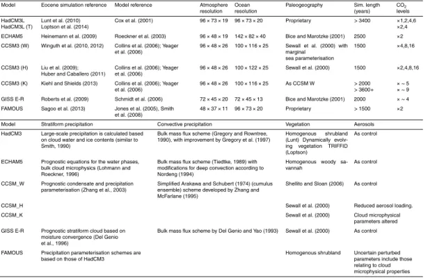
simulated within diﬀ_{erent models has not yet been assessed. Lunt et al. (2012)}

under-took a model intercomparison of early Eocene warmth, EoMIP, based on an ensemble

5

of 12 Eocene simulations undertaken in four fully-coupled atmosphere–ocean climate

models, a summary of which is given in Table 1. This demonstrated diﬀ_{erences in global}

surface air temperature of up to 9◦C for a single imposed CO2and diﬀering regions of

CO2-induced warming, but the implications for the hydrological cycle have not been

considered.

10

This study addresses three main questions: (1) how do globally averaged GCM pre-cipitation rates for the Eocene compare to preindustrial simulations and vary between models in the EoMIP ensemble? (2) How consistently do the EoMIP GCMs simulate

regional precipitation andP−Edistributions? (3) Do diﬀ_{erences between models a}ﬀ_ect

the degree of match with existing proxy estimates for mean annual precipitation?

15

2 Model descriptions

The EoMIP approach of Lunt et al. (2012) is distinct from formal model intercomparison projects which utilise a common experimental design (e.g. PMIP3, Taylor et al., 2012;

CMIP5, Braconnot et al., 2012). Instead, the EoMIP models diﬀ_{er in their boundary}

conditions and span a plausible early Eocene CO2 range, utilise diﬀerent

paleogeo-20

graphic reconstructions and specify diﬀ_{erent vegetation distributions. This is in addition}

to internal diﬀ_{erences in model structure and physics, including precipitation-relevant}

parameterisations such as those relating to convection and cloud microstructure. Whilst

this may hinder the identification of reasons for inter-model diﬀ_{erences, the ensemble}

spans more fully the uncertainty in boundary conditions, which is appropriate for

deep-25

(8)

CPD

11, 3277–3339, 2015

cycle

Title Page

Tables Figures

◭ ◮

Back Close

Full Screen / Esc

Discussion

P

a

per

|

Discussion

P

a

per

|

Discussion

P

a

per

|

Discussion

P

a

per

The ensemble, summarised in Table 1, includes a range of published simulations of the early Eocene carried out with fully dynamic atmosphere–ocean GCMs. We extend the EoMIP ensemble as originally described by Lunt et al. (2012) to include simulations published by Sagoo et al. (2013), Kiehl and Shields (2013) and Loptson et al. (2014). A brief description of each model and the corresponding simulation is given below.

5

Each model produces large-scale (stratiform) and convective precipitation separately, also summarised in Table 1.

2.1 HadCM3L

HadCM3L is a version of the GCM developed by the UK Met Oﬃ_{ce (Cox et al., 2000).}

Eocene simulations performed with atmospheric CO2 at ×2,×4 and ×6 preindustrial

10

levels were presented by Lunt et al. (2010) in their study of the role of ocean circulation as a possible PETM trigger via methane hydrate destabilisation. In these simulations, models were integrated for more than 3400 years to allow intermediate-depth ocean

temperatures to equilibrate. Both the atmosphere and ocean are discretised on a 3.75◦

longitude×2.5◦ latitude grid, with 19 vertical levels in the atmosphere and 20 in the

15

ocean. Vegetation is set to a globally homogenous shrubland.

The eﬀ_{ect of using an interactive vegetation model, TRIFFID (Cox, 2001), on}

temper-ature proxy-model anomalies was considered by Loptson et al. (2014) who performed

simulations at×2 and×4 CO2, continuations of those of Lunt et al. (2010). This study

indicated that for a given prescribed CO2, the inclusion of dynamic vegetation acts to

20

warm global climate via albedo and water vapour feedbacks. We refer to these

simu-lations as HadCM3L_T. The eﬀ_{ect of dynamic vegetation on precipitation distributions}

(9)

CPD

11, 3277–3339, 2015

cycle

Title Page

Tables Figures

◭ ◮

Back Close

Full Screen / Esc

Discussion

P

a

per

|

Discussion

P

a

per

|

Discussion

P

a

per

|

Discussion

P

a

per

2.2 FAMOUS

FAMOUS is an alternative version of the UK Met Oﬃ_{ce’s GCM, adopting the same}

climate parameterisations as HadCM3L, but solved at a reduced spatial and temporal resolution in the atmosphere (Jones et al., 2005; Smith et al., 2008). Atmospheric

reso-lution is 7.5◦longitude×5◦latitude, with 11 levels in the vertical, whilst the ocean

resolu-5

tion matches that of HadCM3L. Both modules operate at an hourly time-step. Because of its reduced resolution, FAMOUS has been used for transient simulations with long run-times and in perturbed parameter ensembles where a large number of simulations are required (Smith and Gregory, 2012; Williams et al., 2013). Sagoo et al. (2013) used

FAMOUS to study the eﬀ_{ect of parametric uncertainty on early Eocene temperature}

10

distributions by varying 10 climatic parameters which are typically poorly constrained in climate models. Their results demonstrated that a globally warm climate with a

re-duced equator-to-pole temperature gradient can be achieved at 2×preindustrial CO2.

Of the seventeen successful simulations which ran to completion, our focus is on E16 and E17, the simulations with the shallowest equator-to-pole temperature gradient and

15

which show the optimal match to marine and terrestrial temperature proxy-data. At the ocean grid resolution, the paleogeography matches that of Lunt et al. (2010). Vege-tation is set to a homogenous shrubland. All simulations were run for a minimum of 8000 model years and full details of the perturbed parameters are provided in Sagoo et al. (2013). Sagoo et al. show DJF and JJA precipitation distributions for their globally

20

warmest and coolest simulations, but comparisons to other models or to proxy data have not been made.

2.3 CCSM3

We utilise three sets of simulations performed with CCSM3, a GCM developed by the US National Centre for Atmospheric Research in collaboration with the university

com-25

(10)

CPD

11, 3277–3339, 2015

cycle

Title Page

Tables Figures

◭ ◮

Back Close

Full Screen / Esc

Discussion

P

a

per

|

Discussion

P

a

per

|

Discussion

P

a

per

|

Discussion

P

a

per

to terrestrial proxy data in a study of the early Eocene climate equability problem by

Huber and Caballero (2011). These simulations are configured with atmospheric CO2

at×2, ×4, ×8 and×16 preindustrial. Models were integrated for between 2000 and

5000 years, until the sea surface temperature was in equilibrium. The atmosphere is

resolved on a 3.75◦ longitude by ∼3.75 latitude (T31) grid with 26 levels in the

ver-5

tical and the ocean is resolved on an irregularly spaced dipole grid. The prescribed land surface cover follows the reconstructed vegetation distribution utilised in Sewall et al. (2000). Following the approach of Lunt et al. (2012) we refer to these simulations as CCSM3_H.

The second set of simulations, which we refer to as CCSM3_W, were described by

10

Winguth et al. (2010) and Shellito et al. (2009) and conducted at×4,×8 and×16

prein-dustrial CO2. Relative to the CCSM3_H simulations, these simulations utilised a

so-lar constant reduced by 0.44 %, were integrated for a shorter period (∼1500 years),

adopted an updated vegetation distribution (Shellito and Sloan, 2006) and utilised

a marginal sea parameterisation, resulting in paleogeographic diﬀ_{erences, particularly}

15

in polar regions. However, the major diﬀ_{erence between the simulations is that the}

CCSM3_W simulations utilise a modern-day aerosol distribution, whereas CCSM3_H adopts a reduced loading for the early Eocene based on a hypothesised lower early Eocene ocean productivity (Kump and Pollard, 2008; Winguth et al., 2012). However, the extent to which increased volcanism at the PETM might have increased aerosol

20

loading remains uncertain (Svensen et al., 2004; Storey et al., 2007).

The third set of simulations, CCSM3_K, are described in Kiehl and Shields (2013). This study investigated the sensitivity of Eocene climatology to the parameterisation

of aerosol and cloud eﬀ_{ects, specifically by altering cloud microphysical parameters}

including cloud drop number and eﬀ_{ective cloud drop radii. Modern day values from}

25

pristine regions are applied homogenously across land and ocean. Simulations were performed at two greenhouse gas concentrations corresponding to possible pre- and

trans-PETM atmospheric compositions which are equivalent to CO2of∼ ×5 and∼ ×9

(11)

CPD

11, 3277–3339, 2015

cycle

Title Page

Tables Figures

◭ ◮

Back Close

Full Screen / Esc

Discussion

P

a

per

|

Discussion

P

a

per

|

Discussion

P

a

per

|

Discussion

P

a

per

as those used in CCSM3_W and the solar constant is reduced by 0.487 % relative to

modern. Changes in precipitation distribution between high- and low-CO2 simulations

have previously been shown for the CCSM3_W and CCSM3_K simulations (Winguth et al., 2010; Kiehl and Shields, 2013), but how robust these Eocene distributions are to GCM choice remains unknown.

5

2.4 ECHAM5/MPI-OM

The ECHAM5/MPI-OM model is the GCM of the Max Planck Institute for Meteorology (Roeckner et al., 2003), used by Heinemann et al. (2009) in their study of reasons for

early Eocene warmth. The model was configured with CO2 at×2 preindustrial, using

the paleogeography of Bice and Marotzke (2001) and a globally homogenous

vegeta-10

tion cover, with lower albedo but larger leaf area and forest fraction than pre-industrial, equivalent to a modern day woody savannah. Atmosphere components are resolved

on a gaussian grid with a spacing of 3.75◦ longitude and approximately 3.75◦latitude.

Relative to the preindustrial simulation, methane is increased from 65 to 80 ppb and nitrous oxide from 270 to 288 ppb for the Eocene, but these are negligible relative to

15

change in radiative forcing associated with doubling of preindustrial CO2. Latitudinal

precipitation distributions in the simulation relative to preindustrial were considered by Heinemann et al. (2009) and elevated convective precipitation at high-latitudes sug-gested to be consistent with convective clouds as a high latitudes warming mechanism (Abbot and Tziperman, 2008).

20

2.5 GISS-ER

The E-R version of the Goddard Institute for Space Studies model (GISS-ER; Schmidt et al., 2006) was utilised by Roberts et al. (2009) in their study of the impact of Arctic paleogeography on high latitude early Eocene sea surface temperature and salinity. Here, we include the simulation with open Arctic paleogeography of Bice and Marotzke

25

(12)

CPD

11, 3277–3339, 2015

cycle

Title Page

Tables Figures

◭ ◮

Back Close

Full Screen / Esc

Discussion

P

a

per

|

Discussion

P

a

per

|

Discussion

P

a

per

|

Discussion

P

a

per

with CO₂at 4×preindustrial, and CH4at 7×preindustrial, equivalent of a total Eocene

greenhouse gas forcing of ∼4.3×preindustrial CO2. The atmospheric component of

GISS-ER has a grid resolution of 4◦latitude by 5◦longitude with 20 levels in the vertical;

the ocean model is of the same horizontal resolution but with 13 levels. Vegetation is prescribed as in Sewall et al. (2000). The hydrological cycle is shown to be intensified

5

for the Paleogene simulation, with elevated global precipitation and evaporation rates, but spatial precipitation distributions were not studied.

3 Results

3.1 Preindustrial simulations

The simulation of precipitation is a particular challenge for GCMs given the range of

10

spatial and temporal scales at which precipitation-producing processes occur, com-pared to a typical model grid and timestep (e.g. Knutti and Sedlacek, 2013; Hage-mann et al., 2006). Model resolution and the parameterisation schemes which account

for sub-grid scale precipitation, in addition to temperature distributions, diﬀ_{er between}

the GCMs in the ensemble (Table 1). We initially summarise model skill in simulating

15

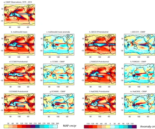
preindustrial Mean Annual Precipitation (MAP) to provide context for our Eocene model intercomparison and to identify which, if any, precipitation structures are unique to the Eocene, and which are more fundamentally related to errors particular to a given GCM. Figure 1 shows preindustrial MAP distributions for each GCM in the EoMIP ensemble and anomalies for each preindustrial simulation relative to CMAP observations

(Cen-20

tre for Climate Prediction, Merged Analysis of Precipitation), which incorporates both satellite and gauge data (Yin et al., 2004; Gruber et al., 2000). The following observa-tions can be made:

i. All of the EoMIP GCMs simulate the principal features of the observed preindus-trial MAP distribution, although errors occur in their position and strength. The

25

(13)

CPD

11, 3277–3339, 2015

cycle

Title Page

Tables Figures

◭ ◮

Back Close

Full Screen / Esc

Discussion

P

a

per

|

Discussion

P

a

per

|

Discussion

P

a

per

|

Discussion

P

a

per

stracks and subtropical precipitation minima in eastern ocean basins are

identifi-able for each simulation, but diﬀ_{erences are evident between the models. Some}

biases are common to a number of the models, in particular those relating to the ITCZ and tropical precipitation. HadCM3L, FAMOUS, ECHAM5 and CCSM3 all simulate the ITCZ mean annual location north of the Equator, but the South

Pa-5

cific Convergence Zone (SPCZ) generally extends too far east in the Pacific, and is too zonal, with precipitation equalling that to the north of the Equator to produce a “double-ITCZ” – a common bias in GCMs (Dai, 2006; Randall et al., 2007). The localised rain belt minimum is a result of the Pacific cold-tongue, not present in GISS-ER, which instead simulates a single convergence zone with high mean

an-10

nual precipitation across the tropics. Other biases which appear common across the ensemble include over-precipitation in the Southern Ocean and too little pre-cipitation over the Amazon and Antarctica (Hack et al., 2006; Randall et al., 2007 and references therein).

ii. Errors over the continents are less than those over the oceans. Absolute errors

15

in MAP are largest over the high precipitation tropical and subtropical oceans,

and frequently exceed 150 cm year−1_{in the case of ITCZ and SPCZ o}_ﬀ_{sets. Over}

the continents, anomalies are generally no greater than 60 cm year−1 and more

than 80 % of the multimodel mean terrestrial surface has an anomaly less than

30 cm year−1_{. In low precipitation regions, these errors could still result in}

signifi-20

cant percentage errors (Fig. S1).

iii. Models show regional diﬀ_{erences in precipitation skill. Figure 1 demonstrates that}

some precipitation biases are individual to particular GCMs. Whilst these are most

noticeable over the high precipitation tropical and subtropical oceans, such as oﬀ

-sets in the location of maximum precipitation intensity or strength of storm tracks,

25

relative diﬀ_{erences within low-precipitation continental regions can also be}

(14)

CPD

11, 3277–3339, 2015

cycle

Title Page

Tables Figures

◭ ◮

Back Close

Full Screen / Esc

Discussion

P

a

per

|

Discussion

P

a

per

|

Discussion

P

a

per

|

Discussion

P

a

per

the study of paleoclimates are also likely to show significant regional diﬀ_{erences in}

their precipitation distribution, underlining the importance of model intercompari-son. Figure 2 additionally shows that all of the EoMIP models simulate a global precipitation rate which agrees fairly well with observational data sets for prein-dustrial climatology (CMAP, GPCP, Legates and Willmott, 1990). Given that all of

5

the models simulate the principal features of MAP distribution, we carry all forward to our Eocene analysis.

3.2 Sensitivity of the global Eocene hydrological cycle to greenhouse gas

forcing

The EoMIP model simulations were configured with a range of plausible early Eocene

10

and PETM atmospheric CO₂ levels, yielding a range of global mean surface air

tem-peratures (Lunt et al., 2012). It is therefore possible to evaluate how consistently

pre-cipitation rates are simulated across the GCMs (i) for a given CO2, (ii) for a given global

mean temperature, or in the case of those models for which multiple simulations have

been performed, (iii) for a given CO2 change and (iv) for a given global mean

tem-15

perature change. Closure of the GCM global hydrological budget requires that total annual precipitation and evaporation are equal, providing there is no net change in

wa-ter storage – the imbalances, summarised in Table S1 are<0.01 mm day−1

equivalent. In HadCM3L, the interannual range in global annual mean precipitation rate across the

95 years over which mean climatology is averaged is 0.07 and 0.06 mm day−1in the×2

20

and ×6 CO2 simulations, respectively, such that the maximum global annual

precipi-tation rate in the timeseries is less than 2.5 % above the minimum rate. We therefore consider mean annual precipitation rate to be a robust estimate of the overall sensitiv-ity of the simulated hydrological cycle. Precipitation rates calculated from three modern observational datasets are shown in Fig. 2b (open circles) and are in relatively good

25

(15)

CPD

11, 3277–3339, 2015

cycle

Title Page

Tables Figures

◭ ◮

Back Close

Full Screen / Esc

Discussion

P

a

per

|

Discussion

P

a

per

|

Discussion

P

a

per

|

Discussion

P

a

per

All of the EoMIP models exhibit a more intense hydrological cycle for the Eocene (Fig. 2b; squares) compared to that simulated in the corresponding preindustrial

sim-ulations (Fig. 2b; circles). For a given CO2, the models vary in the intensity of the

hydrological cycle they simulate – for example, ECHAM5 has a global precipitation rate

at 2×preindustrial CO2comparable to that of CCSM3_W at∼12×preindustrial CO2.

5

In the remainder of this section, we discuss reasons for these diﬀ_{erences, which can}

be attributed to (i) diﬀ_{erences in global/regional temperatures between the simulations,}

(ii) diﬀ_{erences in Eocene boundary conditions, (iii) variation of poorly constrained}

pa-rameter values and (iv) more fundamental diﬀ_{erences in the ways in which the models}

simulate hydrology.

10

The GCMs within the EoMIP ensemble diﬀ_{er in their global mean temperature for}

a given CO2(e.g. Lunt et al., 2012; Fig. 2a). Consequently, the global precipitation rate

for each ensemble member is shown in Fig. 2c relative to its globally averaged sur-face air temperature. This demonstrates that much of the variation between models in

precipitation rate arises from these temperature diﬀ_{erences. For example, the elevated}

15

precipitation rate in the 2×CO2ECHAM5 is explained by this model’s warmth, being

globally>5◦_{C warmer than HadCM3L at the same CO}

2. Similarly, the enhanced

pre-cipitation rate in the CCSM3_K simulations at both∼ ×5 CO2and∼ ×9 CO2relative to

those simulated in CCSM3_H and CCSM3_W are attributable to warmer surface tem-peratures in CCSM3_K, resulting from alterations to cloud condensation nuclei (CNN)

20

parameters, with a reduction in low-level cloud acting to increase short-wave heating at the surface (Kiehl and Shields, 2013). The reduced aerosol loading in CCSM3_H results in surface warming relative to CCSM3_W (Fig. 2a), which explains much of the

7–8 % increase in strength of the hydrological cycle across the CO2range studied; the

×4 CO2simulation in CCSM3_W has approximately the same surface temperature as

25

CCSM3_H at×2 CO2. There are eﬀects beyond those induced by surface

(16)

re-CPD

11, 3277–3339, 2015

cycle

Title Page

Tables Figures

◭ ◮

Back Close

Full Screen / Esc

Discussion

P

a

per

|

Discussion

P

a

per

|

Discussion

P

a

per

|

Discussion

P

a

per

sult of modified aerosol-cloud interactions due to the changes in prescribed aerosols in CCSM_H.

The degree to which the global hydrological cycle will intensify with future global warming has received much attention (e.g. Allen and Ingram, 2002; Held and Soden,

2006; Trenberth, 2011). Held and Soden (2006) show a∼2 % increase in global

pre-5

cipitation per degree of warming for AR4 GCMs forced with the A1B emissions

sce-nario, but with notable inter-model variability. For those simulations with multiple CO₂

forcing, it is possible to estimate how this sensitivity varies for the Eocene. We show

the dP/dT relationships for each model as well as the increase in % precipitation for

a 1◦C temperature increase over the range of 15–30◦C (Table 2). Both CCSM3 and

10

HadCM3L appear to be broadly comparable at∼1.8–2.1 % increase in the intensity of

the hydrological cycle for each degree of warming, consistent with the future climate simulations.

Some variation in the intensity of the hydrological cycle simulated by the EoMIP mod-els may be expected to occur independently of global mean surface air temperature.

15

For preindustrial conditions, boundary conditions are largely constant (atmospheric composition, continental positions, orography and ice sheet distribution), yet the

simu-lations show a spread of∼0.30 mm day−1 – which exceeds the precipitation increase

for a doubling of CO2 from×2 to×4 preindustrial in both CCSM3_H (0.13 mm day−

1

)

and HadCM3L (0.18 mm day−1_{) – these di}_ﬀ_{erences are not explained by di}_ﬀ_erences

20

in preindustrial temperature (Fig. 2b) but may relate to more fundamental diﬀ_erences

in model physics, particularly between HadCM3L and CCSM3W, where a more ac-tive hydrological cycle is consistently simulated in HadCM3L for both the Eocene and preindustrial conditions.

For both the×2 and×4 CO2simulations, the HadCM3L simulations that include the

25

TRIFFID dynamic vegetation model have a near identical precipitation rate to those

without (Fig. 2b). However, the×4 CO2simulation with dynamic vegetation is

substan-tially warmer than the×4 simulation with fixed homogenous shrubland. The inclusion of

(17)

CPD

11, 3277–3339, 2015

cycle

Title Page

Tables Figures

◭ ◮

Back Close

Full Screen / Esc

Discussion

P

a

per

|

Discussion

P

a

per

|

Discussion

P

a

per

|

Discussion

P

a

per

et al. (2014), but this does not yield an associated increase in precipitation. This may

be related to the fact that temperature diﬀ_{erences induced by TRIFFID are}

concen-trated over the land surface, where the evapotranspiration rate is limited by moisture availability. The TRIFFID simulations therefore exhibit a reduced hydrological

sensitiv-ity of∼1.3 % increase in precipitation per degree of warming (dP/dT) compared with

5

∼1.8 % for the non-TRIFFID simulations.

In the FAMOUS simulations undertaken by Sagoo et al. (2013; Fig. 2d), all

simu-lations are performed at 2×CO2, but global temperatures range between 12.3 and

31.8◦C on account of simultaneous variation of 10 uncertain parameter values, some

of which directly influence cloud formation and precipitation. Within these simulations

10

there is also a linear relationship between surface air temperature and global

precip-itation (R2=_0.965; _n=_{17) suggesting the global intensity of the hydrological cycle}

remains primarily coupled to global temperature, despite greater scatter around the

dP/dT relationship. Despite this, the overall dP/dT relationship in FAMOUS is higher

than that of HadCM3L and HadCM3L+_{TRIFFID, with an} _∼_{2.8 % increase in}

precipi-15

tation for each degree of warming (Table 2).

In HadCM3L, the 1×CO2Eocene and preindustrial simulations have similar global

precipitation rates (Fig. 2a), implying that Eocene boundary conditions other than CO2

do not exert a major influence on the intensity of the hydrological cycle, raising global

precipitation rate by only ∼0.10 mm day−1. However, this increase is consistent with

20

and likely driven by a small increase in global surface air temperature. Furthermore, the preindustrial simulations for both CCSM3 and HadCM3L lie on, or close to, the

Eocene-derived dP/dT lines (Fig. 2c), suggesting that globally, precipitation rate for

a given temperature is not increased/decreased for the Eocene, despite diﬀ_{erences in}

low-latitude land–sea distribution, ocean gateways and a lack of Eocene ice sheets.

25

Intriguingly, extrapolating the dP/dCO₂ relationship backwards to 1×CO2 for

CCSM_W would require an Eocene precipitation rate ∼7 % above that of the

prein-dustrial rate. This suggests a more substantial eﬀ_{ect of Eocene boundary conditions}

(18)

CPD

11, 3277–3339, 2015

cycle

Title Page

Tables Figures

◭ ◮

Back Close

Full Screen / Esc

Discussion

P

a

per

|

Discussion

P

a

per

|

Discussion

P

a

per

|

Discussion

P

a

per

still operating via temperature eﬀ_{ects. GISS-ER has a marginally more vigorous}

hydro-logical cycle than the other models for a given global temperature. Roberts et al. (2009)

show that the global precipitation rate in a preindustrial 4×CO2simulation in GISS-ER

is∼4 % greater than that of the preindustrial, whereas the Paleogene simulation has

a precipitation rate∼23 % above that of the preindustrial. Therefore Paleogene

bound-5

ary conditions other than CO2are crucial in elevating precipitation rate in this model.

3.3 Variability in Mean Annual Precipitation (MAP) distribution

3.3.1 Spatial distribution of MAP

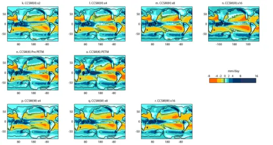
Figure 3 shows MAP distributions for each EoMIP simulation. Eocene distributions are relatively similar to those for preindustrial conditions (Fig. 1), with clearly

recognis-10

able inter-tropical convergence zone (ITCZ), South Pacific convergence zone (SPCZ) and subtropical precipitation minima, the distributions of which appear to be long-standing characteristics of Cenozoic precipitation. Relative to preindustrial simulations, the Eocene distributions exhibit increased precipitation at high latitudes as a conse-quence of elevated Eocene temperatures in these regions. In CCSM in particular, the

15

Eocene is characterised by a more globally equable precipitation rate: the expansion of zones of highest precipitation in the Eocene relative to preindustrial is muted compared with a more extensive loss of low precipitation regions. Additional support for this is pro-vided by a comparison of mean precipitation rates for land and ocean (Table S2). The preindustrial ratio of land : ocean precipitation is maintained in the Eocene HadCM3L

20

and ECHAM simulations, whereas in CCSM, precipitation rates over land and ocean

are typically equal. The eﬀ_{ects of di}ﬀ_{erences in simulated surface air temperatures}

between models within the ensemble are also evident: for a given global surface tem-perature, HadCM3L maintains cooler poles than CCSM3 and ECHAM5 (Sect. 3.3.2)

and regions with MAP<300 cm year−1 persist in the Arctic and Antarctic even at ×4

25

(19)

CPD

11, 3277–3339, 2015

cycle

Title Page

Tables Figures

◭ ◮

Back Close

Full Screen / Esc

Discussion

P

a

per

|

Discussion

P

a

per

|

Discussion

P

a

per

|

Discussion

P

a

per

Modelled Eocene MAP features are frequently traceable to those identified in predin-dustrial simulations (Sect. 3.1), including the single tropical convergence zone in the

GISS×4 CO2simulation and the double ITCZ in a number of the models. Elsewhere,

the Eocene precipitation distributions diverge from those of the preindustrial

simula-tions and may be related to specific Eocene paleogeography, elevated CO2, or other

5

boundary conditions. In HadCM3L, there is a clear trend towards a more south-easterly

trending SPCZ in the higher CO₂simulations, which is not replicated in the warm

sim-ulations of the sister model FAMOUS. The SPCZ in CCSM is also far weaker in the Eocene simulations, compared to preindustrial simulations. Despite similar preindus-trial precipitation distributions over tropical Africa, CCSM and HadCM3L strongly

di-10

verge in the Eocene, with CCSM showing far more intense equatorial precipitation. The FAMOUS simulations E16 and E17 represent two realisations of very warm cli-mates with a reduced equator-pole temperature gradient – in these simulations signifi-cant increases in mid-latitude precipitation are particularly accentuated over the Pacific

Ocean; increases in convection in the subtropics and mid-latitudes are suﬃ_{cient to}

15

eliminate the precipitation minima seen in other models at these latitudes.

For a given CO₂, diﬀ_{ering boundary conditions and simulated model air temperatures}

prevent direct assessment of whether Eocene regional precipitation distributions are robust to GCM selection. We show a multimodel mean in Fig. 5 for simulations with a common global precipitation rate. Elevated high-latitude precipitation for the early

20

Eocene relative to preindustrial conditions is robust between GCMs, although absolute values remain variable between models, particularly in the Southern Hemisphere likely

due to diﬀ_{ering Antarctic orography. Di}ﬀ_{erences between models in the mid-latitudes}

are smaller, resulting in some confidence that the secondary precipitation maxima were polewards of their preindustrial location during the Eocene. Equatorial precipitation

25

(20)

CPD

11, 3277–3339, 2015

cycle

Title Page

Tables Figures

◭ ◮

Back Close

Full Screen / Esc

Discussion

P

a

per

|

Discussion

P

a

per

|

Discussion

P

a

per

|

Discussion

P

a

per

3.3.2 Controls on precipitation distribution

Precipitation rates for each simulation are summarised in Table S2, including separate rates calculated over land and ocean surfaces and rates deconvolved into those arising from convective and large-scale contributions. These data show that elevated

precip-itation rates in the high CO2 Eocene simulations are largely the result of increased

5

convection, although in the ECHAM5 model a greater percentage of precipitation is generated by large scale mechanisms in both the Eocene and preindustrial simulation. Figure 4 shows how convective and large-scale precipitation rates vary with latitude for

a selection of the EoMIP simulations. This reveals diﬀ_{erences between models in the}

mechanisms responsible for precipitation distributions which can be related to surface

10

air temperature distributions. In the HadCM3L simulations, the mid-latitude maxima in

both large scale and convective precipitation advance polewards with increasing CO2

with precipitation increases over the high northern latitudes driven almost exclusively by enhanced large-scale precipitation. CCSM3 has substantially warmer poles which results in much enhanced high-latitude large scale precipitation relative to HadCM3L,

15

although large scale latitudinal contributions diﬀ_{er somewhat for preindustrial}

simula-tions at both low and high latitudes. In CCSM3_K, the warmest CCSM3 simulasimula-tions, polar temperatures are elevated compared to CCSM3_H as is total precipitation in these regions, but in this case large scale precipitation is reduced over much of the high latitudes and the higher total precipitation is due to convective processes.

20

In the warmest FAMOUS simulations of Sagoo et al. (2013), the high latitudes ex-perience particularly significant increases in large scale precipitation, such that the maximum values are those at the poles in the E17 simulation, and in the Southern Hemisphere the local mid-latitude precipitation maximum is lost. Elevated mid lati-tude temperatures in the warm FAMOUS simulations additionally result in significant

25

(21)

CPD

11, 3277–3339, 2015

cycle

Title Page

Tables Figures

◭ ◮

Back Close

Full Screen / Esc

Discussion

P

a

per

|

Discussion

P

a

per

|

Discussion

P

a

per

|

Discussion

P

a

per

of the underlying parameter configuration; this emphasises the fundamental control of

temperature distribution on precipitation, as opposed to the eﬀ_{ect of alteration of any}

one specific parameter.

For HadCM3L and CCSM3, simulations at diﬀ_{erent CO}

2provide an insight into how

regional Eocene precipitation distributions are impacted by warming, and anomaly

5

plots for high – low CO2 simulations are shown in Fig. 6. For the same CO2

forc-ing, CCSM3 is globally cooler than HadCM3L (Lunt et al., 2012), but the anomalies for

16 – 4 CO2 (CCSM_W) and 6 – 2 CO2 (HadCM3L) display similar global changes in

both temperature and therefore precitation rate on account of similar dP/dT

relation-ships (Fig. 2; Table 2). Intriguingly, HadCM3L displays far greater spatial contrasts in

10

net precipitation change, particularly over the ocean: between the pair of HadCM3L simulations, some 23 % of the Earth’s surface experiences an increase or decrease

in precipitation greater than 60 cm year−1, compared to just 6 % in the CCSM3

simu-lations. Some spatial patterns are robust between models – including the dipole-like pattern over the Pacific, SPCZ migration, and subtropical reductions in precipitation

15

at the expense of greater moisture transport to higher latitudes. Other changes are model dependent: in HadCM3L, there is a clear increase in the strength of storm tracks along the eastern Asian coastline, which is not repeated in CCSM. In HadCM3L, addi-tional decreases in precipitation occur around the Peri-Tethys and along the coastline of equatorial Africa. Whilst models within the EoMIP ensemble therefore show

similar-20

ities in their global rate of precipitation change with respect to temperature, regional precipitation distributions are strongly model dependent, diverging within the EoMIP ensemble according to surface air temperature characteristics.

3.4 Precipitation seasonality

The evolution and timing of the onset of global monsoon systems in the Eocene has

25

been the subject of debate (Licht et al., 2014; Sun and Wang, 2005; Wang et al.,

2013). Proxy studies for the early Eocene have highlighted diﬀ_{erences in precipitation}

(22)

CPD

11, 3277–3339, 2015

cycle

Title Page

Tables Figures

◭ ◮

Back Close

Full Screen / Esc

Discussion

P

a

per

|

Discussion

P

a

per

|

Discussion

P

a

per

|

Discussion

P

a

per

et al., 2012) and possible changes to seasonality at the PETM have also been invoked in a number of studies (Sluijs et al., 2011; Schmitz and Pujalte, 2007; Handley et al., 2012). Previous modelling work utilising CCSM3 has suggested that much of the mid-late Eocene was monsoonal, with up to 70 % of annual rainfall occurring during one extended season in North and South Africa, North and South America, Australia and

5

Indo-Asia (Huber and Goldner, 2012). GCMs have been shown to diﬀ_{er greatly in their}

prediction of future monsoon systems (e.g. Turner and Slingo, 2009; Chen and Bordoni,

2014) so we examine the similarities and diﬀ_{erences in Eocene models with respect to}

the seasonality of their precipitation distributions.

Figure 7 shows the percentage of precipitation falling in the extended summer

sea-10

son (MJJAS for Northern Hemisphere; NDJFM for Southern Hemisphere) following the approach of Zhang and Wang (2008) and also utilised in the Eocene studies of Huber and Goldner (2012) and Licht et al. (2014). This metric has been shown to correlate well with the modern-day distribution of monsoon systems. Overall, the models show

a global distribution of early Eocene monsoons in high CO2climates that is similar to

15

those simulated under preindustrial simulations (Fig. S6). Australia is markedly less monsoonal than in preindustrial simulations due to its more southerly Eocene paleolo-cation. Note that regions where winter season precipitation dominates fall at the lower end of the scale; these tend to be over the ocean surface but also include regions around the Peri-Tethys and both the Pacific and Atlantic US coasts.

20

HadCM3L is notable in that it is more seasonal at high latitudes, simulating an early Eocene monsoon centred over modern day Wilkes’ Land region of Antarctica. Although proxy data have suggested highly seasonal precipitation regimes for both the Arctic (Schubert et al., 2012) and Antarctic (Jacques et al., 2014) during this interval, these

systems are maximised in the×2 CO2simulation and weaken somewhat in the

simu-25

lations with elevated CO₂. This arises due to the high temperature seasonality of

Arc-tic/Antarctic Eocene regions in HadCM3L relative to the other models (e.g., Gasson

et al., 2013). In austral winter, Antarctic temperatures are suﬃ_{ciently low to suppress}

(23)

CPD

11, 3277–3339, 2015

cycle

Title Page

Tables Figures

◭ ◮

Back Close

Full Screen / Esc

Discussion

P

a

per

|

Discussion

P

a

per

|

Discussion

P

a

per

|

Discussion

P

a

per

which produce more equable rainfall. The eﬀ_{ect of elevated global warmth on the extent}

of Eocene monsoons is additionally consistent across the models, with a decline in

ter-restrial areas with seasonal precipitation regimes at higher CO2 simulations (Table 3).

HadCM3L simulates a 6 % reduction in the extent of terrestrial regions influenced by

monsoonal regimes for HadCM3L×1 CO2relative to the preindustrial simulation, which

5

appears to be related to the warmer surface temperatures and absence of Antarctic ice sheet.

3.5 P−Edistributions

The diﬀ_{erence between precipitation and evaporation (}_P₋_E_{) is important to consider in}

the characterisation of an enhanced Eocene hydrological cycle. Over land, this

param-10

eter broadly determines the precipitation available to become soil water and surface

runoﬀ_{, the partitioning itself being dependent on the land surface schemes within the}

models (e.g. Cox et al., 1998; Oleson et al., 2004). Over the ocean,P−E drives

dif-ferences in salinity which can aﬀ_{ect the Eocene ocean circulation (Bice and Marotzke,}

2001; Waddell and Moore, 2008). We show mean annual (P −E) budgets for each

15

of the EoMIP simulations in Fig. 8. In warmer climates, an exacerbation of existing

(P −E) is expected – that is, the wet become wetter and the dry drier, as the

mois-ture fluxes associated with existing atmospheric circulations intensify (Held and Soden, 2006). Broadly, the EoMIP simulations support this paradigm for the Eocene relative to preindustrial (Fig. 5). CCSM3 shows fairly minor changes in the boundaries between

20

net-precipitation and net-evaporation zones at higher CO₂ (Fig. 8), although the

net-evaporation zones in HadCM3L do migrate polewards over the eastern Pacific and

North Atlantic at high CO2. Other dynamic changes within HadCM3L are coupled to

the precipitation responses: the more meridionally-orientated SPCZ results in a weaker zonally averaged Southern Hemisphere evaporative zone (Fig. 9) and the expansion

25

of precipitation along the Asian coastline results in a more positive (P −E) balance in

this region. Over continents the models also display diﬀ_{erent responses. Over}

(24)

CPD

11, 3277–3339, 2015

cycle

Title Page

Tables Figures

◭ ◮

Back Close

Full Screen / Esc

Discussion

P

a

per

|

Discussion

P

a

per

|

Discussion

P

a

per

|

Discussion

P

a

per

simlations, driven by increases in precipitation coupled to reductions in evaporation. In CCSM3, the net moisture balance is less responsive with respect to temperature, although instense equatorial precipitation means this region is much wetter than in HadCM3L.

Because of the large latent heat fluxes involved in evaporation and condensation,

5

the global hydrological cycle acts as a meridional transport of energy. Net evapora-tion in the subtropics stores energy in the atmosphere as latent heat, releasing it at high latitudes via precipitation (Pierrehumbert, 2002). An intensified hydrological cycle, associated with increased atmospheric transport of water vapour has therefore been suggested as a potential mechanism for reducing the equator-pole temperature

gradi-10

ent during greenhouse climates (Ulfnar et al., 2004; Caballero and Langen, 2005). By

integrating the area-weighted estimates ofP−Ewith latitude, we show how these

con-tributions diﬀ_{er between the EoMIP models and associated preindustrial simulations in}

Fig. 9. Relative to preindustrial climatology, the intensification of the hydrological cycle associated with increased drying in the net-evaporative zones and increased

moist-15

ening of the net-precipitation zones implies a stronger latent heat flux and within the EoMIP ensemble, the implied polewards energy fluxes of the E16 and E17 FAMOUS

simulations and×2 CO2 ECHAM simulation are particularly significant. GISS-ER has

a particularly strong low latitude equatorially-directed latent heat transfer which arises from the much elevated Eocene precipitation rate in the deep tropics. At face value,

20

it may seem that the elevated latent heat transport at mid to high latitudes could con-tribute towards the reduced equator-pole temperature gradient in the EoMIP simutions, but we note that theoretical and modelling based studies suggest increased la-tent heat transport is associated with an increased equator-pole temperature gradient (Pagani et al., 2014). Within the EoMIP ensemble, meridional temperature gradients

25

and global surface air temperatures covary and so it is not possible to separate clearly

the eﬀ_{ects of these di}ﬀ_{erent controls (Fig. S3). Nevertheless, these results illustrate that}

relative to preindustrial, the Eocene hydrological cycle acts as to elevate the meridional

(25)

CPD

11, 3277–3339, 2015

cycle

Title Page

Tables Figures

◭ ◮

Back Close

Full Screen / Esc

Discussion

P

a

per

|

Discussion

P

a

per

|

Discussion

P

a

per

|

Discussion

P

a

per

4 Proxy-model comparison

A range of proxy data provide constraints on how the early Eocene hydrological cycle

diﬀ_{ered to that of the modern, including oxygen isotopes from mammalian, fish and}

foraminiferal fossils (Clementz and Sewall, 2011; Zachos et al., 2006; Zacke et al., 2009) and the distribution of climatically sensitive sediments (e.g. Huber and

Gold-5

ner, 2012). Changes in regional hydrology at the PETM have also been inferred from geomorphological (John et al., 2008; Schmitz and Pujalte, 2007), biomarker (Hand-ley et al., 2011; Pagani et al., 2006) and microfossil (Sluijs et al., 2011; Kender et al., 2012) proxies. These have often resulted in qualitative interpretations of hydrological change, although the climatic variables and temporal signal they proxies record are

10

uncertain in many instances (e.g. Handley et al., 2011, 2012; Tipple et al., 2013; Sluijs et al., 2007). However, quantitative estimates of Mean Annual Precipitation (MAP), de-rived from micro- and macro-floral fossils have been made for a number of early Eocene and PETM-aged sections which can be compared directly with the GCM-estimated pre-cipitation rates described in Sect. 3.

15

Paleoprecipitation estimates are primarily produced by two distinct paleobotanic methods – leaf physiogonomy and Nearest Living Relative (NLR) approaches. In the former, empirical univariate and multivariate relationships have been established be-tween the size and shape of modern angiosperm leaves and the climate in which they grow, with smaller leaves predominating in low precipitation climates (e.g. Wolfe, 1993;

20

Wilf et al., 1998; Royer et al., 2005). The NLR approach estimates paleoclimate by assuming fossilised specimens have the same climatic tolerances as their presumed extant relatives. This approach can utilise pollen, seeds and fruit in addition to leaf fossils (Mosbrugger et al., 2005). Relative to Mean Annual Temperature, geologic es-timates of MAP are less precise, which may relate to decoupling between MAP and

25

(26)

CPD

11, 3277–3339, 2015

cycle

Title Page

Tables Figures

◭ ◮

Back Close

Full Screen / Esc

Discussion

P

a

per

|

Discussion

P

a

per

|

Discussion

P

a

per

|

Discussion

P

a

per

Our data compilation is provided in Table S3. Some of the data has been compared previously with precipitation rates from an atmosphere-only simulation performed with

isoCAM3 for the Azolla interval (∼49 Ma; Speelman et al., 2010). Our proxy-model

comparison includes data for the remainder of the early-mid Eocene, including a num-ber of recently-published estimates such that the geographic spread is widened to

in-5

clude estimates from Antarctica (Pross et al., 2012), Australia (Contreras et al., 2013; Greenwood et al., 2003), New Zealand (Pancost et al., 2013), South America (Wilf et al., 2005) and Europe (Eldrett et al., 2014; Mosbrugger et al., 2005; Geisental et al., 2011). We select Ypresian-aged data where multiple Eocene precpitation rates exist, including estimates for the PETM but have additionally included some Lutetian and

Pa-10

leocene data, particularly in regions where Ypresian data does not exist. This approach

is justified given the range of plausible Eocene CO2with which simulations have been

performed.

Figure 10 shows paleobotanical estimates for MAP for a range of the data in Ta-ble S2, along with model-estimated rates for each of the EoMIP simulations. Mean

15

precipitation estimates from each model are derived by averaging over grid boxes cen-tred on the paleolocation in a similar approach to Speelman et al. (2010). This is a nine

cell grid of 3×3 gridboxes for HadCM3L, GISS, ECHAM and CCSM3, although in some

instances an eight cell grid of 2×4 is used along paleocoastlines. Diﬀering model

reso-lutions and land–sea masks result in averaging signals from slightly diﬀ_erent

paleogeo-20

graphic areas, but this approach allows for an assessment of the regional signal and error bars are included to show the range of precipitation rates present within the locally defined grid. In the reduced resolution model, FAMOUS, mean and range are derived

from 2×2 gridboxes to ensure regional climatologies remains comparable. Error bars

on the geologic data are generally provided as described in the original publications,

25

with further details also provided in Table S3.

Our results confirm diﬀ_{erent regional sensitivities across the models. Over New}

Zealand (Fig. 10b), HadCM3L shows a strong sensitivity to increases in CO2, whereas