Abstract—This transform was introduced in the year 1997 by Rajan [2], [4] and [5] on the lines of Hadamard Transform. This paper presents, in addition to its formulation, the algebraic properties of the transform and uses in pattern recognition, the technology related to object recognition, that is, about the use of Rajan Transform (RT) in recognizing regular and irregular objects. Rajan Transform is a homomorphism that maps a set consisting of a number sequence, its graphical inverse and their cyclic and dyadic permutations, to a set consisting of a unique number sequence ensuring the invariance property under such permutations. This paper describes in detail the techniques of using RT for recognizing regular and irregular shape objects.
Index Terms— Image processing, Object Recognition, Pattern
classification, Homomorphic Transform
I. INTRODUCTION
Pattern recognition is essentially a classification process. It is after a prolonged research and study of related techniques like Permutation Invariant Systems and Number Theory, Rajan Transform was introduced in the year 1997 as a novel algorithm for classification purposes, which was earlier known as Rapid Transform. Subsequent research on the algebraic properties of this transform has exposed its richness. The purpose of this paper is to present a comprehensive introduction to RT and its algebraic properties, and its role in developing high-speed algorithms for recognizing regular and irregular shape objects. Basically any shape could be described in terms of certain regular shapes defined in a 3X3 neighborhood structure in the manner how an arbitrary signal
Manuscript received July 17, 2006. This work was supported technically and financially by Pentagram Research Centre (P) Limited, 201, Venkat Homes, MIGH – 59, Hyderabad, Andhra Pradesh, India. The authors express their thanks to the University of Mysore, Karnataka, India and MGNIRSA, Hyderabad, India for their administrative support in carrying out this research. *1 Mandalapu Ekambaram Naidu is Professor, TRR Engineering College,, Hyderabad, India, Research Scholar of the University of Mysore, MG-NIRSA, of Dr. Swaminadhan Research Foundation, Hyderabad, Andhra Pradesh, India. E-mail: [email protected]
*2 E. G. Rajan is Professor and Dean, Gokaraju Rangaraju Institute of Engineering & Technology, Hyderabad, President, Pentagram Research Foundation, An Undertaking of Pentagram Research Centre (P) Limited, India. E-mail: [email protected]
is expressed in terms of the orthogonal functions of sinusoidal and co-sinusoidal functions as a power series (Fourier series) consisting of weighted sinusoids and co-sinusoids.
Signal processing is either carried out in time domain or frequency domain depending on the needs and requirement. Similarly shape processing (recognition) is carried out on the representative polygons (similar to frequency components) using Rajan Transform. This paper is intended to present comprehensive details about the state-of-the-art technique of recognizing shapes of objects by analyzing representative polygons.
II. RAJAN TRANSFORM
Rajan Transform is essentially a fast algorithm developed on the lines of Decimation-In-Frequency (DIF) Fast Fourier Transform algorithm, but it is different from the DIF-FFT algorithm. Given a number sequence x(n) of length N, which is a power of 2, first it is divided into the first half and the second half each consisting of (N/2) points so that the following hold good.
g(j) = x(i)+x(i+(N/2)) ; 0 ≤ j ≤ N/2 ; 0 ≤ i ≤ N/2 h(j) = |x (i) – x(i-N/2) )| ; 0 ≤ j ≤ N/2 ; (N/2) ≤ i ≤ N Now each (N/2)–point segment is further divided into two halves each consisting of (N/4) points so that the following hold good.
g1(k) = g(j) + g(j + (N/4)) ; 0≤ k≤ (N/4) ; 0≤ j≤ (N/4)
g2(k) = |g(j) - g(j -(N/4))|;0≤ k≤(N/4);(N/4)≤j≤ (N/2)
h1(k) = h(j) + h(j + (N/4)); 0≤ k≤ (N/4) ; 0≤ j≤ (N/4)
h2(k) = |h(j) -h(j - (N/4))|;0≤ k≤ (N/4);(N/4)≤ j≤ (N/2)
This process is continued till no more division is possible. The total number of stages thus turns out to be log2N. Let us denote
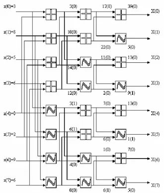
the sum and difference operators respectively as + and ~. If x(n) is a number sequence of length N = 2k; K>0, then its Rajan Transform is denoted as X(k). RT is applicable to any number sequence and it induces an isomorphism in a class of sequences, that is, it maps a domain set consisting of the cyclic and dyadic permutations of a sequence on to a range set consisting of sequences of the form X(k)E(r) where x(k) denotes the permutation invariant RT and E(r) an encryption code corresponding to an element in the domain set. This map is a one-to-one and on to correspondence and an inverse map also exists. Hence it is viewed as a transform. Consider a sequence x(n) = 3, 8, 5, 6, 0, 2, 9, 6. Then X(k) = 39, 5, 13, 9,
Two Dimensional Object Recognition
Using Rajan Transform
Mandalapu Ekambaram Naidu
1, E. G. Rajan
213, 1, 7, 5. The signal flow graph for this transform together with the encryption key (number 0 or 1 inside the brackets) is given in figure 2.1.
Fig. 2.1: Signal flow diagram of one-dimensional 8-point RT
Observe from the diagram that E(r) is a union of three sequences E1(r) = 0, 0, 0, 0, 1, 1, 0, 0 , E2(r) = 0, 0, 0, 0, 0, 0, 0,
1 and E3(r) = 0, 0, 0, 1, 0, 1, 0, 0. That is, E(r) = E1(r)E2(r)E3(r).
Now, the sequence X(k)E(r) = 39, 5, 13, 9, 13, 1, 7, 5, 0, 0, 0, 0, 1, 1, 0, 0, 0, 0, 0, 0, 0, 0, 0, 1, 0, 0, 0, 1, 0, 1, 0, 0 is the RT of the input sequence x(n) = 3, 8, 5, 6, 0, 2, 9, 6. In general, the first point in a RT is called ‘Cumulative point Index’ (CPI).
III. INVERSE RAJAN TRANSFORM
Retrieval of the information or the signal x(n) can be done by Inverse Rajan Transform (IRT) [2], [4] and [5]. The basic requirements for the IRT computation are the RT coefficients associated with the encryption values (k values) that are generated by encryption function while computing forward RT. The strategy adopted here is to retrace the forward transform signal flow graph. It was observed that the point-wise addition of a constant value, say K to the sample sequence x(n) while computing forward RT, changes only the DC component X0,
that is, the CPI to X0+NK, which is the first coefficient of the
newly computed RT, and the remaining spectral values remain the same of the original spectrum. For example, the RT spectrum X(k) of the sequence x(n) = 3, 8, 5, 6, 0, 2, 9, 6 is 39, 5, 13, 9, 13, 1, 7, 5. Now let us build a new sequence x1(n) = 4,
9, 6, 7, 1, 3, 10, 7 by adding K=1 to the sequence x(n) = 3, 8, 5, 6, 0, 2, 9, 6. The RT spectrum of the new sequence is X1(k) =
47, 5, 13, 9, 13, 1, 7, 5. Now, in order to work with sequences containing negative sample values, we proceed as usual in the case of forward transform. But, the inverse transform is
calculated just by adding a constant value N(2M-1) to the CPI value of the spectrum. M is the bit length required to represent the maximum quantization level of the samples and N is the length of the sequence. This constant factor K = (2M-1) is chosen such that all the maximum possible negative values of the sequence x(n) are level shifted to 0 or above. This DC shift is required, because we hide the sign of the negative values that are generated while computing the forward RT. As mentioned earlier, RT induces an isomorphism between the domain set consisting of the inverse, cyclic, dyadic and dual class permutations of a sequence on to a range set consisting of sequences of the form X(k)E(r) where X(k) denotes the permutation invariant RT and E(r) an encryption code corresponding to an element in the domain set. This map is a one-to-one and on-to correspondence and an inverse map also exists. Thus RT is viewed as a transform. Now we provide a technique for obtaining the inverse of Rajan Transform. Inverse Rajan transform (IRT) is a recursive algorithm and it transforms a RT code X(k)E(r) of length N(1+m) where N = 2m and m is the number of stages of computation, into one of its original sequences belonging to its permutation class depending on the encryption code E(r). The computation of IRT is carried out in the following manner. First the input sequence is divided into segments each consisting of two points so that either
g(2j+1) = (X(2k)+X(2k+1))/2
g(2j) = max (X(2k), X(2k+1))-g(2j+1);
if E1 (2r)= 0 and E1(2r+1) = 0; 0≤j<N; 0≤k≤N; 0≤r≤N,
or g(2j) = (X(2k)+X(2k+1))/2
g(2j+1) = max (X(2k), X(2k+1) - g(2j)
if E1 (2r) = 1 or E1 (2r+1) = 1; 0≤j≤N; 0≤ k≤N; 0≤r≤N.
The resulting sequence is divided into segments each consisting of four points. Each 4-point segment is synthesized as per the above procedure. The resulting sequence is further divided into segments each consisting of eight points and the same procedure is carried out. This process is continued till no more division is possible. Consider X(k) = 39,5,13,9,13,1,7,5. Then its IRT is x(n) = 3, 8, 5, 6, 0, 2, 9, 6. The inverse x(n) is obtained from the given X(k)E(r) as shown in figure 3.1.
The symbols ^ > and ~ respectively denote the operators average of two, maximum of two and difference of two. Note that IRT will work only in the presence of encryption sequence E(r) and for every member of the permutation class there would be a unique encryption sequence. Study of the class of encryption sequences corresponding input sequences itself is a field of active research. A specific example would make things easy. Let us consider a sequence x(n) = 3, 8, 5, 6, 0, 2, 9, 6 and its RT, X(k) = 39, 5, 13, 9, 13, 1, 7, 5. Now addition of 15 to each sample point in x(n) would yield a sequence x1(n) = 18,
23, 20, 21, 15, 17, 24, 21 and its RT would be X1(k) = 159, 5,
13, 9, 13, 1, 7, 5. Observe that X1(0) = X(0) + 120 = 39 + 120 =
obtain the actual sample domain sequence. Let us take the case of X(k) = 39, 5, 13, 9, 13, 1, 7, 5. Now let us add 120 only to X(0) so that the spectral sequence becomes 159, 5, 13, 9, 13, 1, 7, 5. The IRT of this sequence is 18, 23, 20, 21, 15, 17, 24, 21. By subtracting 15 from each sample value we obtain the actual sequence 3, 8, 5, 6, 0, 2, 9, 6.
Fig.3.1: Signal flow diagram of IRT of a spectral sequence
IV. ALGEBRAIC PROPERTIES OF RAJAN TRANSFORM
RT has interesting algebraic properties like permutation invariance, scalar property and linear pair forming property. All such properties are explained in short in the following.
Cyclic shift invariance property
Let us consider the same sequence x(n) = 3,8,5,6,0,2,9,6. Using this sequence one can generate seven more cyclic shifted versions such as xc1(n) = 6, 3, 8, 5, 6, 0, 2, 9 , xc2(n) = 9, 6, 3, 8,
5, 6, 0, 2 , xc3(n) = 2, 9, 6, 3, 8, 5, 6, 0 , xc4(n) = 0, 2, 9, 6, 3, 8, 5,
6 , xc5(n) = 6, 0, 2, 9, 6, 3, 8, 5 , xc6(n) = 5, 6, 0, 2, 9, 6, 3, 8 and
xc7(n) = 8, 5, 6, 0, 2, 9, 6, 3. It is obvious that the cyclic shifted
version of xc7(n) is x(n) itself. One can easily verify that all
these eight sequences have the same X(k), that is, the sequence 39, 5, 13, 9, 13, 1, 7, 5 but different E(r).
Graphical inverse invariance property
The sequence x(n) = 3, 8, 5, 6, 0, 2, 9, 6 has the graphical inverse x-1(n) = 6, 9, 2, 0, 6, 5, 8, 3. Using this sequence one can generate seven more cyclic shifted versions such as xc1-1(n) = 3, 6, 9, 2, 0, 6, 5, 8 , xc2-1(n) = 8, 3, 6, 9, 2, 0,
6, 5 , xc3-1(n) = 5, 8, 3, 6, 9, 2, 0, 6 , xc4-1(n) = 6, 5, 8, 3, 6, 9, 2, 0
, xc5-1(n) = 0, 6, 5, 8, 3, 6, 9, 2 , xc6-1(n) = 2, 0, 6, 5, 8, 3, 6, 9 and
xc7-1(n) = 9, 2, 0, 6, 5, 8, 3, 6. It is obvious that the cyclic
shifted version of xc7-1(n) is x-1(n) itself. One can easily verify
that all these eight sequences have the same X(k), that is, the sequence 39, 5, 13, 9, 13, 1, 7, 5 but different E(r)
D y a d i c s h i f t i n v a r i a n c e p r o p e r t y
T h e t e r m ‘ d y a d ’ r e f e r s t o a g r o u p o f t w o , a n d t h e t e r m ‘ d y a d i c s h i f t ’ t o t h e o p e r a t i o n o f t r a n s p o s i t i o n o f t w o b l o c k s o f e l e me n t s i n a s e q u e n c e . F o r i n s t a n c e , l e t u s t a k e x ( n ) = 3 , 8 , 5 , 6 , 0 , 2 , 9 , 6 a n d t r a n s p o s e i t s f i r s t h a l f w i t h t h e s e c o n d h a l f . T h e r e s u l t i n g s e q u e n c e Td( 2 )[ x ( n ) ] = 0 , 2 , 9 , 6 ,
3 , 8 , 5 , 6 i s t h e 2 - b l o c k d y a d i c s h i f t e d v e r s i o n o f x ( n ) . T h e s y mb o l Td( 2 ) d e n o t e s t h e 2 - b l o c k d y a d i c
s h i f t o p e r a t o r . I n t h e s a me ma n n e r , w e o b t a i n Td( 4 )[ Td( 2 )[ x ( n ) ] ] = 9 , 6 , 0 , 2 , 5 , 6 , 3 , 8 a n d
Td( 8 )[ Td( 4 )[ Td( 2 )[ x ( n ) ] ] ] = 6 , 9 , 2 , 0 , 6 , 5 , 8 , 3 . O n e
c a n e a s i l y v e r i f y t h a t a l l t h e s e d y a d i c s h i f t e d s e q u e n c e s h a v e t h e s a me X ( k ) , t h a t i s , t h e s e q u e n c e 3 9 , 5 , 1 3 , 9 , 1 3 , 7 , 5 b u t d i f f e r e n t E ( r ) . There is yet another way of dyadic shifting the input sequence x(n) to Td( 2 )[Td( 4 )[Td( 8 )[x(n)]]]. Let us take x(n) = 3, 8, 5, 6, 0, 2, 9, 6
and obtain the following dyadic shifts: Td( 8 )[x(n)] = 8, 3, 6, 5,
2, 0, 6, 9 , Td( 4 )[Td( 8 )[x(n)]] = 6, 5, 8, 3, 6, 9, 2, 0 and
Td( 2 )[Td( 4 )[Td( 8 )[x(n)]]] = 6, 9, 2, 0, 6, 5, 8, 3. Note that
Td( 2 )[Td( 4 )[Td( 8 )[x(n)]]] = Td( 8 )[Td( 4 )[Td( 2 )[x(n)]]]. One
can easily verify from the above that other than Td( 4 )[Td( 2 )[x(n)]] and Td( 8 )[x(n)], all other dyadically
permuted sequences fall under the category of the cyclic permutation class of x(n) and x-1(n). This amounts to saying that the cyclic permutation class of x(n) has eight non-repeating independent sequences, that of x-1(n) has eight non-repeating independent sequences and the dyadic permutation classes of x(n) has two non-repeating independent sequences. To conclude, all these 18 sequences could be seen to have the same X(k). Each of these 18 sequences has an independent encryption key E(r).
Dual class invariance
Given a sequence x(n), one can construct another sequence y(n) consisting of at least one number which is not present in x(n) such that X(k) = Y(k). In such a case, y(n) is called the dual of x(n). An arbitrary sequence x(n) of length N=2n is said to have a dual y(n) if and only if its CPI is an even number and is divisible by N/2. In other words, x(n) is said to form a dual pair with y(n). Consider two sequences x(n) = 2, 4, 2, 2 and y(n) = 3, 1, 3, 3. Note that X(k) = Y(k) = 10, 2, 2, 2 and the point-wise mean of the two sequences x(n) and y(n) is 2.5. From a dual pair one can generate another sequence (child sequence) consisting of numbers which are point-wise differences of the pair. Duality is a hereditary property that is transferred to child sequences.
Regenerative property
value 5. Now one can obtain the dual sequence y(n) = 2, 4, 2, 2 by subtracting each element of x(n) from 5. Now x(n) and y(n) form a pair and yield their ‘first generation child sequence’, say x1(n) = 1, 3, 1, 1 , which is obtained by finding the point wise
difference between the parent sequences x(n) and y(n). One can easily verify that x1(n) also is eligible to form a dual pair with
y1(n) = 2, 0, 2, 2. This hereditary property is termed here as
‘regenerative property’. Another important observation follows. x1(n) forms a dual pair with y1(n) but this pair does not
produce a child sequence as it was done by the pair <x(n), y(n)>.This could be easily verified by the fact that the point wise difference between x1(n) and y1(n) yields x1(n) only.
Hence for brevity we call the sequences x1(n) and y1(n) as
‘sterile sequences’ and the pair <x1(n), y1(n)> as a ‘sterile pair’.
This property opens up new avenues for further research on generative and sterile pairs which have potential applications to areas related to encryption, and cryptography..
Scalar property
Let x(n) be a number sequence and A be a scalar. Then the RT of Ax(n) will be AX(k), where X(k) is the RT of x(n). For example, let us consider a sequence x(n) = 1, 3, 1, 2 and a scalar A of value 2. Now the RT X(k) of x(n) is 7, 3, 1, 1. The RT of Ax(n) = 2, 6, 2, 4 is 14, 6, 2, 2 which is nothing but AX(k).
Linearity property
In general, RT does not satisfy the linearity property. However, it was observed that for a pair x(n) and y(n) which are number sequences either in the increasing order or in the decreasing order, the linearity property holds. That is, for Ax(n)+my(n) where A and m are scalars and x(n) and y(n) are two number sequences either in the increasing or decreasing order, the RT will be AX(k)+mY(k), where X(k) and Y(k) are respectively the RTs of x(n) and y(n). A characterization theorem is yet to be established for categorizing pairs of sequences which would satisfy linearity property.
Linear pair forming property
Two sequences x(n) and y(n) are said to form a linear pair when X(k)+Y(k) is the RT of x(n)+y(n), where X(k) and Y(k) are the RTs of x(n) and y(n) respectively. The symbol + denotes the point wise addition of two sequences. As outlined earlier, pairs of sequences consisting of increasing numbers of decreasing numbers only form linear pair. In general arbitrary sequences do not form linear pairs. Consequently RT could be viewed as a nonlinear transform. However, higher order RT spectra do form linear pairs, and this has been identified as a very useful property for pattern recognition purposes.
For instance let us consider two arbitrary sequences x(n) and y(n) given below:
x(n) = 2,2,2,1,6,2,6,1,2,3,0,0,2,5,5,4; (16-point sequence) y(n) = 4,5,3,1,0,1,4,6,6,8,0,0,7,9,0,5; (16-point sequence) Now the RT of x(n) denoted as X1(k) is computed as X1(k) =
43, 7, 7, 5, 19, 7, 7, 3, 15, 1, 1, 1, 9, 1, 3, 3 and the RT of y(n) denoted as Y1(k) is computed as Y1(k) = 59, 11, 21, 1, 17, 9, 9,
5, 29, 3, 11, 7, 11, 1, 9, 1. Now, z(n) = x(n) + y(n) is given by the sequence 6, 7, 5, 2, 6, 3, 10, 7, 8, 11, 0, 0, 9, 14, 16, 6, 8, 6, 8, 6, where as X1(k) + Y1(k) = 102, 18, 28, 6, 36, 16, 16, 8, 34,
4, 12, 8, 20, 2, 12, 4. Note that Z(k) is not equal to X1(k) +
Y1(k). Now, the second order RT spectra of X1(k) and Y1(k) are
respectively computed as X2(k) = 132, 76, 72, 64, 32, 32, 28,
28, 64, 32, 36, 20, 24, 16, 20, 12 and Y2(k) = 204, 128, 76, 56,
80, 68, 48, 44, 72, 20, 32, 20, 36, 32, 16, 12. Let z1(n) be the
sequence X1(k) + Y1(k). Then Z1(k) is the RT of and z1(n) and
is computed to be 326, 194, 138, 110, 98, 86, 70, 66, 138, 70, 86, 42, 66, 62, 42, 38. Note that Z1(k) is not equal to X2(k) +
Y2(k) = 336, 204, 148, 120, 112, 100, 76, 72, 136, 52, 68, 40,
60, 48, 36, 24. This procedure is repeated for the third order spectra as follows: X3(k) = 688, 128, 128, 64, 304, 96, 96, 64,
240, 0, 32, 32, 144, 32, 32, 32 and Y3(k) = 944, 184, 336, 104,
272, 136, 144, 88, 464, 40, 176, 24, 176, 24, 144, 8 are the RTs of X2(k) and Y2(k) respectively. The RT of X2(k) + Y2(k) is
computed to be 1632, 312, 464, 168, 576, 232, 240, 152, 704, 40, 208, 56, 320, 56, 176, 40 which is nothing but X3(k) +
Y3(k).
Thus it is clear from the above example that higher order RT spectra of arbitrary sequences of equal length do form linear pairs, and so the name ‘linear pair forming property’. Linear pair forming property is also called self-organizing property. To be more precise, given any arbitrary random sequence of appropriate length, the successive RTs would introduce order in the sequences and exhibit linearity property.
V. OBJECT RECOGNITION USING RAJAN TRANSFORM
Shape representation
Any regular or irregular object image (two dimensional) could be represented by a set of basis convex polygons that are shown in figure 5.1. The convex polygons are labeled based on the vertices whose cells are dropped. The term `convex polygon’ refers to the polygon which is drawn by connecting the boundary cells and the central cell is not touched by the lines drawn. For example the convex polygon E1,3,5,7 is the polygon
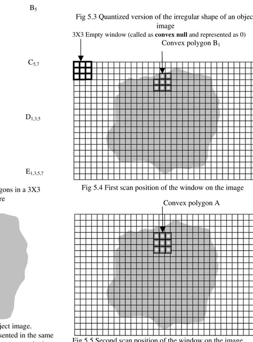
obtained by dropping the cells 1, 3, 5 and 7. Let us consider an irregular shape shown in figure 5.2. The image shown in figure 5.2 is quantized as shown in figure 5.3.
The quantized image is further scanned by the 3X3 neighborhood window and on each move the polygon that could be fitted inside the image is observed. For example the first scan position of the image is shown in figure 5.4. The polygon B1 is found to be contained in the image. The window
A B1 B3 B5
B7 C1,3 C3,5 C5,7
C7,1 C5,1 C7,3 D1,3,5
D3,5,7 D1,5,7 D1,3,7 E1,3,5,7
Fig 5.1: Sixteen basis convex polygons in a 3X3 neighbourhood structure
Fig 5.2 Irregular shape of an object image. Any irregular image could also be represented in the same manner using 16 convex polygons. Now one can apply the Rajan Transform to all these 16 convex polygons as described below.
After scanning the image once by the 3X3 window the scanning window is brought down by one row and the image scanned from left to right. This procedure of raster scanning is continued till the entire image is scanned by the window.
Fig 5.3 Quantized version of the irregular shape of an object image
3X3 Empty window (called as convex null and represented as 0) Convex polygon B1
Fig 5.4 First scan position of the window on the image
Fig 5.5 Second scan position of the window on the image The overall effect of scanning the image yields a string of symbols denoting such convex polygons. This string is called pextral representation of the image just like the notion of spectral representation of a signal. For example, the pextral representation of the image given in figure 5.3 is computed as 073B1A
7 B30
16 B1A
12
016A13016A13B50 15
A14015 A14015A14015A13015B1A
13 B50
12 B1A
15 014B7A
13 B50
15 B7A
12 017AB
7A 10
022B7A 4
B70 70
where the symbol 073 represents a string of 73 convex nulls.
RT spectrum of the pextra of 16 convex polygons
The central idea on which this concept has been developed is the fact that it is sufficient to find the pextrum of a shape by considering the contour of the given shape as a string of 0s and 1s and finding out the RT spectrum of it. For example, let us consider the contour of the pattern represented by the symbol A which is shown in figure 5.6
Convex polygon A
Starting point
Fig 5.6:Binary string representing the boundary of the pattern A
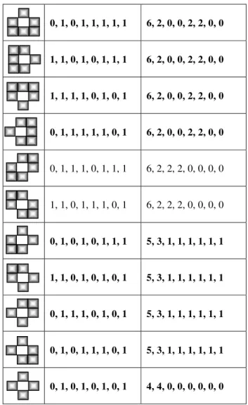
The RT spectrum of this binary string is 8,0,0,0,0,0,0,0. So, the pextrum of the shape A is 8,0,0,0,0,0,0,0. Table 5.1 provides the pextra of all 16 convex patterns.
Now, the RT spectrum of the pextral code 073B1A7B3016B1
A12016A13016A13B5015A14015 A14015 A14 015A13015B1A13B5012
B1A15014B7A13B5015B7A12017AB7A10022B7A4B7070 is 073,7,1,1,
1,1,1,1,1, (8,1,1,1,1,1,1,1)7,7,1,1,1,1,1,1,1,016, 7,1,1,1,1,1,1,1, (8,0,0,0,0,0,0,0)12,016,(8.0.0.0.0.0.0.0)13,016,(8,0,0,0,0,0,0,0)13, 7,1,1,1,1,1,1,1,015,(8,0,0,0,0,0,0,0)14,015,(8,0,0,0,0,0,0,0)14,015, (8,0,0,0,0,0,0,0)14,015,(8,0,0,0,0,0,0,0)13,015,7,1,1,1,1,1,1,1,(8,0 ,0,0,0,0,0,0)13,7,1,1,1,1,1,1,1,012,7,1,1,1,1,1,1,1,(8,0,0,0,0,0,0, 0)15,014,7,1,1,1,1,1,1,1,(8,0,0,0,0,0,0,0)13,7,1,1,1,1,1,1,1, 015,7,1,1,1,1,1,1,1,(8,0,0,0,0,0,0,0)12,017,8,0,0,0,0,0,0,0,7,1,1,1 ,1,1,1,1,(8,0,0,0,0,0,0,0)10,022,7,1,1,1,1,1,1,1,(8,0,0,0,0,0,0, 0)4 ,7,1,1,1,1,1,1,1,070
Object Recognition from RT spectrum of the pextra of 16
convex polygons
The technique of recognizing an object in a two dimanesional digital plane is as follows: The given digital image is represented as a string of the 16 basis convex polygons. Then each of the poygon is numerically coded in terms of 8 bits of 0s and 1s and RT applied to each block of 8 bits. From RT spectrum, one can characterize the shape of a given image. One can as well obtain the histogram of the pextral code and form an idea of the shape of a given image.
Table 5.1: Pextra of all 16 convex patterns Pattern Representative
String
Corresponding Pextrum 1, 1, 1, 1, 1, 1, 1, 1 8, 0, 0, 0, 0, 0, 0, 0
0, 1, 1, 1, 1, 1, 1, 1 7, 1, 1, 1, 1, 1, 1, 1
1, 1, 0, 1, 1, 1, 1, 1 7, 1, 1, 1, 1, 1, 1, 1
1, 1, 1, 1, 0, 1, 1, 1 7, 1, 1, 1, 1, 1, 1, 1
1, 1, 1, 1, 1, 1, 0, 1 7, 1, 1, 1, 1, 1, 1, 1
0, 1, 0, 1, 1, 1, 1, 1 6, 2, 0, 0, 2, 2, 0, 0
1, 1, 0, 1, 0, 1, 1, 1 6, 2, 0, 0, 2, 2, 0, 0
1, 1, 1, 1, 0, 1, 0, 1 6, 2, 0, 0, 2, 2, 0, 0
0, 1, 1, 1, 1, 1, 0, 1 6, 2, 0, 0, 2, 2, 0, 0
0, 1, 1, 1, 0, 1, 1, 1 6, 2, 2, 2, 0, 0, 0, 0
1, 1, 0, 1, 1, 1, 0, 1 6, 2, 2, 2, 0, 0, 0, 0
0, 1, 0, 1, 0, 1, 1, 1 5, 3, 1, 1, 1, 1, 1, 1
1, 1, 0, 1, 0, 1, 0, 1 5, 3, 1, 1, 1, 1, 1, 1
0, 1, 1, 1, 0, 1, 0, 1 5, 3, 1, 1, 1, 1, 1, 1
0, 1, 0, 1, 1, 1, 0, 1 5, 3, 1, 1, 1, 1, 1, 1
0, 1, 0, 1, 0, 1, 0, 1 4, 4, 0, 0, 0, 0, 0, 0
For example, let us consider the example given above. The histogram of the pextral code is shown in figure 5.7.
Fig 5.7: Histogram of the pextral code.
Observations:
The number of 0s, that is, convex polygons in an image indicates a measure of the background of the image, whereas the number of As in an image indicates the area spanned by the image. The presence of other polygons and their actual number gives an approximate nature of the boundary of the image.
Inference
Hence, it is proposed in this paper to study the spectra of the polygons rather than the spectra of the entire image.
VI. C
ONCLUSIONSRajan Transform has been used as a high-speed spectral domain tool to carry out object recognition and digital image processing operations. This paper mainly focuses on algebraic properties of the transform and uses in object recognition from RT spectrum of the pextra of 16 convex polygons. Research carry out so for clearly indicate that RT could be one of the best tools that could be used in cryptography. RT based watermarking of text and images and character recognition would yield a repertoire of tools of the future. Efforts are being made to abstract the notion of RT to Symbolic Processing of Signals and Images in the DNA computing paradigm.
VII. R
EFERENCES[1] Rajan, E G, “Cellular Logic Array Processing Techniques for High-Throughput Image Processing Systems”, Invited paper, SADHANA, Special Issue on Computer Vision, The Indian Academy of Sciences, Vol 18, Part-2, June 1993, pp 279-300.
[2] Rajan, E G, “On the Notion of Generalized Rapid Transformation”, World multi conference on Systemics, Cybernetics and Informatics, Caracas, Venezuela, July 7 – 11, 1997
[3] Rajan, E.G., “Symbolic Computing – Signal and Image Processing”, B.S. Publications, Hyderabad, 2003.
[4] Venugopal S, “Pattern Recognition for Intelligent Manufacturing Systems using Rajan Transform”, MS Thesis, Jawaharlal Nehru Technological University, Hyderabad, 1999.
Prof. M. Ekambaram Naidu obtained his B. Tech degree in Electronics and Communication Engineering from S.V. University, Tirupathi, India, in 1985, M. Tech degree in Computer Science and Engineering from Mangalore University in 1992 and he is in the process of submitting his Ph.D thesis in the Computer Science Department of the University of Mysore, Karnataka, India. He has about 20 years of Industrial, Professional, Teaching and Research experience. His areas of
interest are: Signal and Image Processing, Computer Vision, Pattern Recognition and Analysis, Cybernetics and Informatics, Symbolic Computation, Computer Networks, Software Engineering, Object Oriented Design and Programming. E-mail: [email protected] Mobile: 98492 58356.
Dr. E. G. Rajan is the President of Pentagram Research Centre (P) Limited, Hyderabad, India. He has 31 years of teaching, research and professional experience. He has originated the logico-mathematical paradigm for carrying out signal and image processing. His book on Symbolic Computing–Signal and Image Processing may turn out to be the futuristic computer science paradigm. He is Adviser to Gokaraju Rangaraju Educational Society, Hyderabad and Dean of the School of Computing, Gokaraju Rangaraju Institute of Engineering and Technology, Hyderabad, India.