Article
HYPERSPECTRAL IMAGE DENOISING USING MULTIPLE LINEAR REGRESSION AND BIVARIATE SHRINKAGE WITH 2-D DUAL-TREE
COMPLEX WAVELET IN THE SPECTRAL DERIVATIVE DOMAIN
Remoção de ruído de imagens hiperespectrais usando regressão linear múltipla e
compressão bivariada com transformada complexa de Wavelet de árvore binária
2D no domínio espectral derivado
Lei Sun 1
Dong Xu 1
College of Science, National University of Defence Technology, Changsha, Hunan, P. R. China 1
Email:[email protected]; [email protected].
Abstract:
In this paper, a new denoising method is proposed for hyperspectral remote sensing images, and tested on both the simulated and the real-life datacubes. Predicted datacube of the hyperspectral images is calculated by multiple linear regression in the spectral domain based on the strong spectral correlation of the useful signal and the inter-band uncorrelation of the random noise terms in hyperspectral images. A two dimensional dual-tree complex wavelet transform is performed in the spectral derivative domain, where the noise level is elevated temporarily to avoid signal deformation during the wavelet denoising, and then the bivariate shrinkage is used to shrink the wavelet coefficients. Simulated experimental results demonstrate that the proposed method obtains better results than the other denoising methods proposed in the reference, improves the signal to noise ratio up to 0.5dB to 10dB. The real-life data experiment shows that the proposed method is valid and effective.
Keywords: Hyperspectral imagery, denoising, multiple linear regression, complex wavelet, bivariate shrinkage
Resumo:
possibilita obter resultados melhores do que outros métodos de remoção de ruídos encontrados na literatura, com melhoria da razão de ruído do sinal de 0.5dB para 10dB. Os dados reais utilizados mostraram que o método proposto é válido e efetivo.
.
Palavras-chave: Remoção de ruído de imagem hiperespectral, regressão linear múltipla, wavelet complexa, compressão bivariada.
1. Introdutcion
wavelet transform and considering a local neighborhood during the thresholding process. In this paper the proposed method in (Chen and Qian, 2011) is referred to as PCABS.
Signal-to-noise ratio (SNR) is a key parameter on measuring the hyperspectral image quality. A sufficiently high SNR can be achieved by adopting some excessive measures in the instrument design, such as increasing the size of the optical system, the integration time, or the detector area. However, these measures are prohibitively expensive, particularly in the spaceborne instruments (Chen and Qian, 2011). So noise reduction algorithms provide a high-effective solution which is becoming more and more affordable in terms of computational time and expense, due to the availability of the advanced computing devices. The reference (Chen, et al, 2010) shows that, for 3-D data cube, it is necessary to perform 1-D spectral signature denoising in addition to 2-D denoising for every spectral band. Xu, et al (2013) propose denoising method for hyperspectral remote sensing image based on multiple linear regression and wavelet shrinkage. To get better performance, curvelet transform is employed for hyperspectral image denoising, which overcomes the major drawback that wavelet cannot really represent two-dimensional objects with edges sparsely (Xu, et al, 2013).
In this paper, due to the strong spectral correlation, the multiple linear regression (MLR) and the spectral derivative are employed to remove the one-dimensional spectral noise. Since the predicted datacubes obtained by MLR have a relatively high SNR, the noise is subtle to distinguish from the useful signals. In order to avoid removing the useful signal during the denoising process, the noise level is elevated temporarily by transforming the datacube into the spectral derivative domain. Then two-dimensional dual-tree complex wavelet transform (DTCWT2) is performed on the datacube in the spectral derivative domain and the wavelet coefficients are shrank by bivariate wavelet thresholding to remove the spatial noise.
Mathematical tools applied in this paper are introduced in Section 2. Section 3 proposes the new denoising algorithm. The noise model is given in Section 4, and the simulated and the real-life data experiment are performed. Section 5 draws the conclusion.
2. Mathematical Tools
2.1 MLR Model
Assume that the hyperspectral image has Bspectral bands and each band of hyperspectral image has MN pixels. Let X denote a P B matrix of the B spectral observed vectors of size P ( PMN). The P1vector X (k k1, 2, , )B is the k-th column vector of the matrixX . Namely, lexicographically arranging k-th band image into a column vector Xk. In this paper,
ˆ
Xk is the vector predicted for the signal Xk of band k. The L adjacent bands (not including
itself) are utilized to perform MLR, that is
ˆ
Xk Xkk(k1, 2, , )B (1)
where theP L matrix Xkconsists of the adjacent column vectors of Xk (not including the
-th
k column vector). If L is even, Xkhas the form
2 2
1 1 1 1 2
1 1 2 2
1 1 2
[X , ,X ,X , ,X ] X [X , ,X ,X , ,X ]
[X , ,X ,X , ,X ]
L L
L
k k L
L L
k k k k k
L
B L k k B
k k B
B k B
(2)
If L is odd, Xkhas the form
1 1
2 2
1
1 1 1 1 2
1 1
1 1 1 2 2
1
1 1 2
[X , ,X ,X , ,X ] X [X , ,X ,X , ,X ]
[X , ,X ,X , ,X ]
L L
L
k k L
L L
k k k k k
L
B L k k B
k k B
B k B
(3) k
is the regression vector of size L1. Fork1, 2, ,B, the least squares estimator of the regression vector k is given by
1ˆ X X X X
k k
T T
k k k
(4)
2.2 Spectral derivative domain
It is well known that hyperspectral data in derivative domain is sensitive to noise, but it is relatively less sensitive in the spectral domain (Othman and Qian, 2006; Tsai and Philpot, 1998). Transforming hyperspectral datacube into the spectral derivative domain is equivalent to high-pass filtering, where the noise level is elevated. The derivative of the spectral band image is defined as follows
( , , ) ( , , ) ( , , ) dx i j x i j x i j
d
wherex i j( , , ) stands for the pixel value of the position ( , )i j in spectral band center and is the distance between the adjacent bands. In computation, the equation (5) is also given as follows
( , , ) ( , , 1) ( , , ), 1,2, 1 x i j k x i j k x i j k k B
(6)
wherex i j k( , , )stands for the pixel value of the position ( , )i j in band k, x i j k( , , ) stands for the pixel value of the derivative domain and B is the total number of spectral bands in hyperspectral image.
2.3 2-D dual-tree complex wavelet
Wavelet has a good time-frequency-localization property. As a result of multi-resolution approach, the signal power is concentrated in the low frequency subband by wavelet transform, and the high frequency subband describes non-stationary characteristics of the signal well. However, the real wavelet transform suffers from four fundamental, intertwined shortcomings, which are oscillations, shift variance, aliasing and lack of directionality.
The complex wavelet transform (CWT) is proposed to overcome the four shortcomings. The dual-tree complex wavelet transform (DTCWT) is the relative enhancement to the discrete wavelet transform (DWT) (Selesnick, et al, 2005). Comparing to DWT, DTCWT has two important additional properties, which is nearly shift invariant, and directionally selective in higher dimensions. This means that the squared magnitude of a given complex wavelet coefficient provides an accurate measure of spectral energy at a particular location in space, scale and orientation. The CWT can also give a substantial performance boost to DWT noise reduction algorithms. It also means that CWT-based algorithm will automatically be almost shift invariant, thus reducing many of the artefacts of the critically sampled DWT. And oscillations and aliasing have also been overcome during performing the DTCWT.
The effective performances of several other denoising algorithms using the CWT have also been described in (Sendur and Selesnick, 2002; Ye and Lu, 2003). The CWT obtains better results than the DWT, which is an important reason for using the CWT in this paper.
2.4 Bivariate shrinkage (BS)
In the wavelet domain, we define x11n1 and x22n2, x1 and x2 are noisy observations of
1
and 2 , where 2 is the parent of 1, n1 and n2 are noise samples. The 2-D bivariate
thresholding formula is given by
2 2 3 2
1 2
1 1 2 2
1 2
n
x x x
x x
(7)
where x max , 0 x . The noise variance n can be estimated as n Median(x1i) 0.6745, x1i are the wavelet coefficients at the finest scale, and
1 1
2 2
1
i i
n x S
x M
(8)where M is the number of pixels in the 2-D neighbourhood window S. The size of S is chosen to be 7 7 in terms of denoising performance and computational time.
For the complex-valued coefficients, the real and imaginary parts are not shift invariant individually but their magnitudes are. So when thresholding the complex-valued coefficients of the CWT, it is typically more effective to apply the nonlinearity to the magnitude rather than to the real and imaginary parts separately.
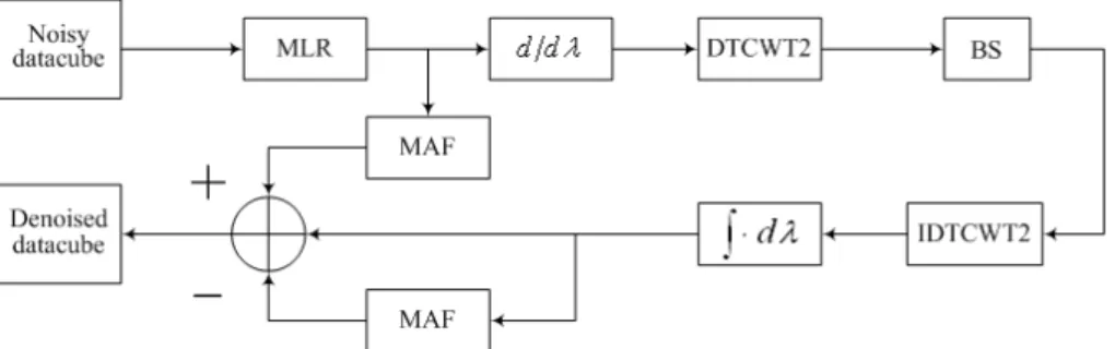
3. Denoising Algorithm
The denoising process is as follows (Figure 1):
(1) The 1-D spectral noise is firstly removed by the MLR, which utilizes L bands (not include itself);
(2) The noise level is elevated temporarily by transforming hyperspectral datacube into the spectral derivative domain;
(3) Performing the 2-D DTCWT (DTCWT2) on each band in the spectral derivative domain;
(4) Bivariate wavelet thresholding is performed to shrink the complex-valued coefficients;
(5) Performing the inverse DTCWT2 (IDCWT2) on the complex -valued coefficients which have been shrank;
Figure 1: Block diagram of the proposed method in this paper
In the last step of the denoising process, the denoised signal x i j kˆ( , , ) is retrieved by spectral
integration (Othman and Qian, 2006)
1
1
( , ,1) 1
ˆ( , , )
ˆ
( , ,1) k ( , , ) 2
l
x i j k
x i j k
x i j x i j l k
(9)where the denoised spectral derivative xˆ is obtained by the inverse DTCWT2 (IDTCWT2). The
process is given by
ˆ IDTCWT2 BS DTCWT2
x x
(10)
According to the equation (9), computational error accumulated due to the integration in the spectral derivative of hyperspectral image after denoising, and the error grows withk. In order to suppress the growing error, the moving average filter (MAF) is applied as shown in Figure 1. The MAF is a simple low-pass filter, and its width of sliding window is 1, which is also named as the correction window. The integration updating process is given by
2 2
2 2
1 1
ˆ ˆ
( , , ) ( , , ) ( , , ) ( , , )
1 1
l k l k
l k l k
x i j k x i j k x i j l x i j l
(11)where x i j k( , , ) is the denoised signal after correction, x i j kˆ( , , ) is the denoised signal before correction, x i j l( , , ) is the noisy signal and 1 is the size of correction window. The reason for
using the noisy signal (instead of the pure signal) is that the pure signal is unknown. The size of correction window is 5.
4. Experimental Results
4.1 Noise Model
A generalized noise model has been proposed to deal with several different acquisition systems. In this paper, we use the following parametric model (Acito, et al, 2011; Alparone, et al, 2009)
( )
y x n x (12)
where y is the observed noisy image, x is the noise-free image, n x( )is the random noise. The noise corresponding to different pixel positions are statistically independent. In equation (12),
( )
n x is composed of both photon and thermal noise and is modeled as a zero mean Gaussian random vector whose covariance matrix depends on the useful signal x. According to the reference (Acito, et al, 2011), the random noise has diagonal covariance matrix whose diagonal entries are the variances of each band
2( ) 1, ,
k xk uk xk wk k B
(13)
where ukxk is regarded as signal-dependent noise and wk is regarded as the signal-independent
noise.
Here, the SNR is defined as follows
X N
SNRP P (14)
where PX is the power of the pure signals x i j k( , , ), and PN is the noise power in the noisy
signalsy i j k( , , ), that is
, , , ,
2 2
1, 1, 1 1, 1, 1
( , , ) ( , , ) ( , , )
M N B M N B
i j k i j k
SNR x i j k y i j k x i j k
(15)N SD SI
P P P (16)
where PSD is the signal-dependent noise power and PSI is the signal-independent noise power, so
we obtain
1
1 1
( )
X
SD SI SD SI
P SNR
P P SNR SNR
(17)
where SNRSD PX PSDand SNRSI PX PSI.
By assuming SNRSI SNRSD , according to equation (15) we obtain
1
(1 )
SD
4.2 Experiment
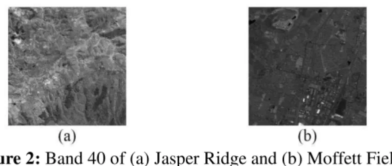
The simulated experiment of the noise reduction is carried out on AVIRIS images, Jasper Ridge and Moffett Field provided by JPL, NASA. The size of datacube is extracted from the AVIRIS images for testing is 256256224 (width height band). Figure 2 shows the image of band 40. For the AVIRIS image a 28m28mground sample distance (GSD) datacube is derived by
spatially averaging the 4m4mGSD datacube elevating the SNR to 38.45dB. Having such high
SNR, this datacube is viewed as a pure datacube (Othman and Qian, 2006), which is used as a reference to measure the SNR before and after denoising. The images are corrupted by noise model described before. In this paper, the SNR of the hyperspectral image for testing is 27.78dB and 30.00dB respectively, and the parameter is chosen to be 0.25, 1 and 4, respectively.
Figure 2: Band 40 of (a) Jasper Ridge and (b) Moffett Field
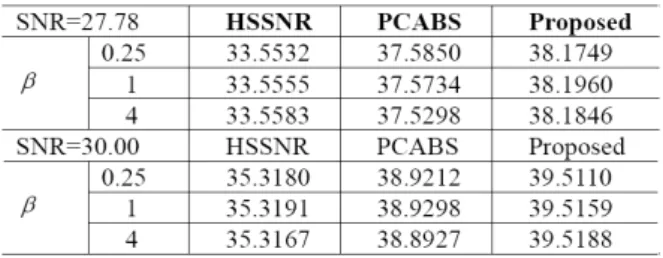
In order to illustrate the superiority of the proposed algorithm in this paper, the proposed method is compared with the algorithm HSSNR proposed in (Othman and Qian,, 2006), and the algorithm PCABS proposed in (Chen and Qian, 2011). In this paper, L is equal to 223, that is, all bands (not including itself) have been utilized to perform MLR. The DTCWT pack is acquired from the web: http://dap.rice.edu/. The types of wavelet are LeGall 5, 3 tap filters and quarter sample shift orthogonal (Q-Shift) 10, 10 tap filters, and the level of decomposition is 6, by which the best results have been obtained. Table 1 and Table 2 show the SNR of the hyperspectral image Jasper Ridge and Moffett Field denoised by the proposed method, the PCABS and the HSSNR. The results of Table 1 and Table 2 indicate that the proposed method is better than the HSSNR method and the PCABS method for hyperspectral image denoising in terms of SNR.
Table 1: SNR of Jasper Ridge by the HSSNR, PCABS, and the proposed algorithm (dB)
We use OMIS (operational modular imaging spectrometer) data developed by the Shanghai Institute of Technical Physics of the Chinese Academy of Sciences for the real-life data experiment to verify the correctness and performance of algorithm. It has 128 spectral bands ranging from visible to thermal infrared wavelength. The size of datacube extracted from OMIS data for testing is 256256128 (width height band). We perform denoising for the original OMIS data. Figure 3 shows band #20, #60 #90 of the original image and the denoised image obtained by PCABS and the proposed method, and the difference between the original image and the denoised image obtained by PCABS and the proposed method in this paper. The difference is considered as the noise removed from the original image. Therefore the less fine details of the image in the difference means the better denoised results. From the Figure 3 (d) and (e), the image (d) contains more fine details than the image (e), which is easy to distinguish by the human eyes. The result shows that the PCABS method removes the finer details during the denoising process. Therefore, the proposed algorithm is superior to the PCABS in terms of removing noise and simultaneously maintaining fine features during the denoising process.
Figure 3: Band #20, #60 #90 of (a) the original image and (b) the denoised image obtained by the PCABS, (c) the denoised image obtained by the proposed method, and (d) the difference between the original image and the denoised image obtained by PCABS, (e) the difference between the original image and the denoised image obtained by the proposed method.
131585.1 11120.1 19140.5 11120.1 4678.7 1671.2 19140.5 1671.2 7851.9
5
.
CONCLUSION
A denoising method of hyperspectral remote sensing image based on the combination of MLR and bivariate shrinkage with 2-D dual-tree complex wavelet transform is proposed in this paper. Due to the strong spectral correlation of the useful signal and the weak spectral correlation of the random noise in hyperspectral images, MLR is employed to decouple the spectral correlation. To elevate the noise level, the hyperspectral image is transformed in the derivative domain. Bivariate shrinkage with dual-tree complex wavelet transform is performed to remove the spatial noise.
In the simulated experiment, AVIRIS images Jasper Ridge and Moffett Field are tested by HSSNR, PCABS and our proposed method. The results show that the all three methods improve the image quality in terms of SNR. For the 27.78dB noisy image, the proposed method improves the SNR up to 10dB, which is about 5dB higher than HSSNR, and 0.5dB to 0.8dB higher than PCABS. For the 30dB noisy image, the proposed method improves the SNR up to 9.5dB to 9.8dB, which is about 4.3dB higher than HSSNR, and about 0.7dB higher than PCABS. Among the three methods, our proposed method performs best in the simulated experiment. For the real-life OMIS data, the experiment results show that our proposed method maintains more fine details of the image during the denoising. This is better than the other two denoising methods which have already proven to perform well in the literature.
AKCNOWLEDGEMENT
This work is supported by the National Natural Science Foundation of China under Project 61101183 and Project 41201363.
REFERENCES
Acito, Nicola, Diani, M., and Corsini, G. “Signal-dependent Noise Modeling and Model Parameter Estimation in Hyperspectral Images” IEEE Transactions on Geoscience and Remote Sensing 49(2011): 2957-2971.
Acito, Nicola, Diani, M., and Corsini, G. “Residual Striping Reduction in Hyperspectral Images.” Paper presented at the 17th International Conference on Digital Signal Processing,
Alparone, Luciano, et al. “Signal-dependent Noise Modelling and Estimation of New-generation
Imaging Spectrometers.” Paper presented at the Hyperspectral Image and Signal Processing: Evolution in Remote Sensing, Grenoble, France, August 26-28, 2009.
Bioucas-Dias, JosÉ M., and Nascimento, J. M. P. “Hyperspectral Subspace Identification.”IEEE Transactions on Geoscience and Remote Sensing 46(2008): 2435-2445.
Chen, Guangyi, Bui T. D., and Krzyzak, A. “Denoising of Three Dimensional Data Cube Using Bivariate Wavelet Shrinking.” Paper presented at the Proc. ICIAR, Povoa de Varzim, Portugal,
June 21–23, 2010.
Chen, Guangyi, and Qian, S. E. “Simultaneous Dimensionality Deduction and Denoising of Hyperspectral Imagery Using Bivariate Wavelet Shrinking and Principal Component Analysis.”
Can. J. Remote Sens. 34 (2008): 447-454.
Chen, Guangyi, and Qian, S. E. “Denoising and Dimensionality Reduction of Hyperspectral Imagery Using Wavelet Packets, Neighbour Shrinking and Principal Component Analysis.” Int. J. Remote Sens. 30 (2009): 4889-4895.
Chen, Guangyi, and Qian, S. E. “Denoising of Hyperspectral Imagery Using Principal Component Analysis and Wavelet Shrinkage.” IEEE Trans. Geosci. Remote Sens. 49 (2011):
973-980.
Donoho, David L. “Denoising by Soft-thresholding.” IEEE Trans. Inform. Theory 41 (1995):
613-627.
Donoho, David L., and Johnstone, I. M. “Ideal spatial adaptation by wavelet shrinkage.” Biometrika 81 (1994): 425–455.
Donoho, David L., and Johnstone, I. M. “Adapting to Unknown Smoothness via Wavelet Shrinkage.”J. Amer. Statist. Assoc. 90 (1995): 1200–1224.
Gao, Lian-Ru, et al. “A New Operational Method for Estimating Noise in Hyperspectral
Images.”IEEE Geoscience and Remote Sensing Letters 5(2008): 83-87.
Green, Andrew A., et al. “A Transformation for Ordering Multispectral Data in Terms of Image
Quality with Implications for Noise Removal.” IEEE Transactions on Geoscience and Remote Sensing 26 (1988): 65-74.
Lee, James B., Woodyatt, A. S., and Berman, M. “Enhancement of High Spectral Resolution Remote Sensing Data by a Noise-adjusted Principal Components Transform.” IEEE Transactions on Geoscience and Remote Sensing 28 (1990): 295-304.
Mihcak, M. Kivanc, et al. “Low Complexity Image Denoising Based on Statistical Modeling of
Wavelet Coefficients.” IEEE Signal Process. Lett. 6(1999): 300–303.
Othman, Hisham, and Qian, S. E. “Noise Reduction of Hyperspectral Imagery Using Hybrid Spatial-spectral Derivative-domain Wavelet Shrinkage.” IEEE Trans. Geosci. Remote Sens. 44
(2006): 397-408.
Roger, R. E., and Arnold, J. F. “Reliably Estimating the Noise in AVIRIS Hyperspectral Images.”International Journal of Remote Sensing 17(1996): 1951-1962.
Selesnick, Ivan, W., Baraniuk, R. G., and Kingsbury, N. G. “The Dual-tree Complex Wavelet Transform.” IEEE Signal Process. 22 (2005): 123-151.
Sendur, Levent, and Selesnick, I. W. “Bivariate Shrinkage Functions for Wavelet Based Denoising Exploiting Interscale Dependency.” IEEE Trans. Signal Process. 50(2002): 2744–
Sendur, Levent, and Selesnick, I. W. “Bivariate Shrinkage with Local Variance Estimation.”
IEEE Signal Process. Lett. 9 (2002): 438–441.
Sun, Lei, and Luo, J. S. “Three-dimensional Hybrid Denoising Algorithm in Derivative Domain for Hyperspectral Remote Sensing Imagery.” Spectroscopy and Spectral Analysis, 29 (2009):
2717-2720.
Tsai, Fuan, and Philpot, W. “Derivative Analysis of Hyperspectral Data.” Remote Sensing of Environment, 66 (1998): 41-51.
Xu, Dong, Sun, L., and Luo, J. “Denoising of Hyperspectral Remote Sensing Image using
Multiple Linear Regression and Wavelet Shrinkage.” Paper presented at the International
Conference on Information, Business and Education Technology, Beijing, China, March 14-15,
2013.
Xu, Dong, et al. “Analysis and Denoising of Hyperspectral Remote Sensing Image in the
Curvelet Domain.” Mathematical Problems in Engineering, 2013(2013): 1-11.
Ye, Zhen, and Lu, C. C. “A complex wavelet domain Markov model for image denoising.” Paper presented at the IEEE Int. Conf. Image Processing, Barcelona, Spain, September 14-17, 2003.