A Longer-run Perspective on Fiscal Sustainability

Carlos Pestana Barros & Nicolas Peypoch

A Comparative Analysis of Productivity Change in Italian and Portuguese Airports

WP 006/2007/DE _________________________________________________________

António Afonso & João Tovar Jalles

A Longer-run Perspective

on Fiscal Sustainability

WP 17/2011/DE/UECE _________________________________________________________

Department of Economics

W

P

ISSN Nº 0874-4548

A Longer-run Perspective on Fiscal

Sustainability

*

July 2011

António Afonso

and João Tovar Jalles

Abstract

This paper investigates the sustainability of fiscal policy in a set of 19 countries by taking a longer-run secular perspective over the period 1880-2009. Via a systematic analysis of the stationarity properties of the first-differenced level of government debt, and disentangling the components of the debt series using Structural Time Series Models, we are able to conclude that the solvency condition would be satisfied in mostly all cases since non-stationarity can be rejected, and, therefore, longer-run fiscal sustainability cannot be rejected (Japan and Spain can be exceptions). The same would be true for the panel sample analysis.

JEL: C23, E62, H62

Keywords: fiscal sustainability, government debt, unit roots, breaks, structural time series models

_____________________________

*

The opinions expressed herein are those of the authors and do not necessarily reflect those of the ECB or the Eurosystem. #

European Central Bank, Directorate General Economics, Kaiserstraße 29, D-60311 Frankfurt am Main, Germany. email: antonio.afonso@ecb.europa.eu.

$

ISEG/UTL - Technical University of Lisbon, Department of Economics; UECE – Research Unit on Complexity and Economics. R. Miguel Lupi 20, 1249-078 Lisbon, Portugal. UECE is supported by FCT (Fundação para a Ciência e a Tecnologia, Portugal). email: aafonso@iseg.utl.pt.

+ _{University of Cambridge, Faculty of Economics, Sidgwick Avenue, Cambridge CB3 9DD, United Kingdom, email:}

Contents

Non-technical summary ... 3

1. Introduction ... 4

2. Theoretical Framework ... 5

3. Empirical Methodology ... 7

3.1 Unit Roots and Structural Breaks ... 7

3.2 Unobserved Components and Structural Time Series Models ... 9

3.3 Panel Unit Roots ... 9

4. Empirical Analysis ... 9

5. Conclusion ... 18

References ... 19

Non-technical summary

The importance of maintaining sustainable fiscal policies has become paramount in the aftermath of the economic and financial crisis in 2008/09. Indeed, maintaining a stable long-term relationship between government expenditures and revenues is one of the key requirements for a stable macroeconomic environment and a sustainable economy. Such is also the challenge of several developed economies, notably in the European Union.

Therefore, the main purpose of this paper is to investigate the sustainability of fiscal policy in a set of 19 countries by taking a longer-run secular perspective covering the period 1880-2009. In addition, in our empirical approach we perform a systematic analysis of the stationarity properties of the first-differenced level of government debt. This approach will provide us with an indirect test on the solvency of public finances in these countries.

Consequently, this paper adds to the existing literature by applying a plethora of different (and recent) unit-root tests to 19 countries using consistent public finance data from one single source that put together the longest government debt database to date. It also tests for the existence of structural breaks during the time sample of each country. By means of Structural Time Series Models allowing for stochastic unobserved components and taking advantage of the long time series we have available, we decompose them into cycle, trend and irregular components, and analyse the evolution and behaviour of the corresponding trend growth over the period under scrutiny.

Via a systematic analysis of the stationarity properties of the first-differenced level of government debt, we are able to conclude that the solvency condition would be satisfied in mostly all cases since non-stationarity can be rejected, and, therefore, longer-run fiscal sustainability cannot (Japan and Spain can be exceptions). In addtion, the implications of the

global _financial crisis for government debt in 2008 and 2009 are also picked up in the

analysis.

1. Introduction

The importance of maintaining sustainable fiscal policies has become paramount in the

aftermath of the economic and financial crisis in 2008/09. Indeed, maintaining a stable

long-term relationship between government expenditures and revenues is one of the key

requirements for a stable macroeconomic environment and a sustainable economy. Such is

also the challenge of several developed economies, notably in the European Union.

Fiscal sustainability is a useful criterion to evaluate whether or not fiscal policy is on a

right long-term track.1 Theoretically, sustainable fiscal policies would need to prevail without

any modification in the existing policy stance, or, in other words, if the intertemporal

government budget constraint holds in present value terms. Conversely, if sound fiscal

policies are absent, economic policies at both macro and microeconomic levels will become

unmanageable and will require policy changes. On the other hand, fiscal sustainability is

challenged when the debt-to-GDP ratio reaches an excessive value, and government revenues

are not enough to keep on financing the new issuance of government debt.

The empirical assessments of fiscal sustainability, stemming from the intertemporal

government budget constraint, usually test for the existence unit roots in government debt and

budget deficit series, and/or for cointegration between government revenues and expenditures.

Such strand of analysis deals with explicit government liabilities.2 _{The empirical studies tend}

to focus mostly looking on the US and on European cases (see, Hamilton and Flavin, 1986;

Hakkio and Rush, 1991; Trehan and Walsh, 1991; MacDonald, 1992; Ahmed and Rogers,

1995; Quintos, 1995; Makrydakis et al., 1999; Feve and Henin, 2000; Martin, 2000; Bravo

and Silvestre, 2002; Hatemi-J, 2002; Afonso, 2005; Mendoza and Ostry, 2007; Arghyrou and

Luintel, 2007, to name a few).

Since fiscal sustainability needs to be tackled at the country level, a country assessment is

naturally necessary. On the other hand, a panel analysis of the sustainability of public finances

is also relevant, notably in the case of the European Union (EU). In this context, recent panel

analysis of fiscal sustainability that has been carried out for the EU, which points to the

solvency of government public finances when considering the EU15, suggesting that fiscal

policy may not have been sustainable for several countries, although it may have been less

unsustainable for some countries (Denmark, Finland, Luxembourg, and the Netherlands).3

_____________________________

1

Analysis on sustainability has focused on both the univariate properties on debt (e.g. Hamilton and Flavin, 1986) and the long-run relationship between revenues and expenditures (e.g. Hakkio and Rush, 1991).

2

See Afonso (2005) for an overview.

3

Still, usually the time spans used, either in country specific analysis or in a panel set up, tend

to go far back as only the 1970s, which can limit the full assessment of long-run fiscal

sustainability.

Therefore, the main purpose of this paper is to investigate the sustainability of fiscal policy

in a set of 19 countries by taking a longer-run secular perspective covering the period

1880-2009. In addition, in our empirical approach we perform a systematic analysis of the

stationarity properties of the first-differenced level of government debt. This approach will

provide us with an indirect test on the solvency of public finances in these countries.

Consequently, this paper adds to the existing literature by applying a plethora of different

(and recent) unit-root tests to 19 countries using consistent public finance data from one

single source, Abbas et al. (2010) who put together the longest government debt database to

date. It also tests for the existence of structural breaks during the time sample of each country.

By means of Structural Time Series Models allowing for stochastic unobserved components

and taking advantage of the long time series we have available, we decompose them into

cycle, trend and irregular components, and analyse the evolution and behaviour of the

corresponding trend growth over the period under scrutiny.

Essentially, our results show that the solvency condition would be satisfied in mostly all

cases since non-stationarity can be rejected. Therefore, longer-run fiscal sustainability cannot

be rejected (Japan and Spain can be exceptions), and the same would be true for the panel

sample analysis.

The structure of the paper is as follows. Section 2 briefly reviews the underlying theoretical

framework, which is the basis for the empirical analysis. Section 3 presents the empirical and

econometric methodology. Section 4 discusses our results and findings. Section 5 concludes.

2. Theoretical Framework

If fiscal developments turn out to be unsustainable, fiscal policy has to guarantee that the

future primary balances are consistent with the intertemporal government budget constraint.4

The hypothesis of fiscal policy sustainability is related to the condition that the trajectory of

the main macroeconomic variables is not affected by the choice between the issuance of

government debt or the increase in taxation. Under such conditions, it would not be crucial

how the deficits are financed, implying also the assumption of the Ricardian Equivalence

hypothesis.5

_____________________________

4

For instance, Cuddington (1997) and Hénin (1997) discuss this topic.

5

One can start with the government budget constraint to derive the present value of the

budget constraint (PVBC). Therefore, the flow budget constraint is written as

t t t t

t r B R B

G +(1+ ) ₋1= + , (1)

where G is the government expenditures, excluding interest payments, R is the government

revenues, B is the government debt and r is the real interest rate.6

Rewriting equation (1) for the subsequent periods, and solving recursively leads to the

intertemporal budget constraint:

∏

∑

∏

j t j

s t s s s j j t s t s t t r B r G R B 1 1 1 ) 1 ( lim ) 1 ( . (2)

When the second term from the right-hand side of equation (2) is zero, the present value of

the existing stock of government debt will be identical to the present value of future primary

surpluses. For empirical purposes it is useful to make several algebraic modifications to

equation (1). Assuming that the real interest rate is stationary, with mean r, and defining

1

)

( − ₋

+

= _{t t t}

t G r r B

E , (3)

it is possible to obtain the following so-called PVBC:

∑

B . (4)

A sustainable fiscal policy should ensure that the present value of the stock of government

debt, the second term of the right hand side of (4), goes to zero in infinity, constraining the

debt to grow no faster than the real interest rate. In other words, it implies imposing the

absence of Ponzi games and the fulfilment of the intertemporal budget constraint. When

facing this transversality condition, the government will have to achieve future primary

surpluses whose present value adds up to the current value of the stock of government debt. In

other words, government debt in real terms cannot increase indefinitely at a growth rate that is

higher than real interest rate.7

A common practice in the literature, among the set of methods to evaluate fiscal policy

sustainability, is to investigate past fiscal data to see if government debt follows a stationary

process.8 Recalling the PVBC, equation (4), it is possible to have two complementary

definitions of sustainability or empirical testing:

i) The value of current government debt equals the sum of future primary budget surpluses:

_____________________________

6 _{Sometimes in the literature the real interest rate is assumed stationary, but this is a much more difficult}

assumption for the nominal interest rate.

7

See McCallum (1984) and Joines (1991).

8

) (

) 1 (

1

0 1

1 t s t s

s s

t R E

r

B _{+ +}

∞

= +

− =

∑

ii) The present value of government debt must approach zero in infinity:

0 ) 1 (

lim ₁ =

+ +

+ ∞

→ s

s t

s _r

B

. (6)

Therefore, and in order to test empirically the absence of Ponzi games, one can test the

stationarity of the first difference of the stock of government debt (∆B_t).

3. Empirical Methodology

3.1 Unit Roots and Structural Breaks

Before disentangling the different components of our government debt series using

Structural Time Series Models (STM), one should formally test the possibility of lasting

shocks in our variables of interest. It is important to be aware of the possibility of a spurious

break phenomenon. Whenever a series is non-stationary, with a unit-root, one or more breaks

may be erroneously suggested by the data even if it is stable over time. This problem was first

raised from a graphic perspective by Hendry and Neale (1991). Therefore, our structural time

series analysis should be complemented by (ex-ante) appropriate statistical hypothesis tests.

Hence, in order to narrow down the number of suitable structural time series models for the

19 countries, some statistics have been computed, which provide additional information in

relation to the main characteristics of the different components of the variable.9 In relation to

the trend of the variables, unit root tests can provide a valuable insight into the presence of

either a deterministic or stochastic secular component in the government debt series. In this

context, in addition to standard Augmented Dickey Fuller (ADF) and Phillips-Perron (PP)

unit root tests – for purposes of robustness and completeness10 – we also conduct the four

tests (M-tests) proposed by Ng and Perron (2001) (NP) based on modified information criteria

(MIC): the modified Phillips-Perron test MZ_α; the modified Sargan-Bhargava test (MSB);

the modified point optimal test MPT; and the modified Phillips-Perron MZT. These tests

improve the PP-tests both with regard to size distortions and power.

In addition, we resort to unit root tests allowing for breaks, notably the Zivot-Andrews

(1992) (ZA) one. This endogenous structural break test is a sequential test which utilizes the

_____________________________

9

The countries are: Argentina, Austria, Belgium, Brazil, Denmark, France, Germany, Greece, Italy, Japan, the Netherlands, New Zealand, Norway, Portugal, Russian Federation, Spain, Sweden, the United Kingdom, and the United States

10

full sample and uses a different dummy variable for each possible break date. The break date

is selected where the t-statistic from the ADF test of unit root is at a minimum (most

negative). Consequently a break date will be chosen where the evidence is least favourable for

the unit root null.11 We complement this with the modified ADF test proposed by Vogelsang

and Perron (1998) (VP) also allowing for one endogenously determined break. Finally, we

also use the two-break unit root test described by Clemente, Montanes and Reyes (1998)

(CMR).12 This latter test tests the null of unit root against the break-stationary alternative

hypothesis and provides us supplementary insights vis-à-vis conventional unit root tests that

do not account for any break in the data.

For the unit root tests that allow for one or two endogenously determined breaks it is

assumed that the shift can be modelled by a dummy variable DUt =0 for t≤TB and for t>TB,

where TB is the shift date (time break). In the time series literature, two generating

mechanisms of shifts are distinguished, additive outlier (AO) and innovational outlier (IO)

models. The former results in an abrupt shift in the level, whereas the latter allows for a

smooth shift from the initial level to a new level. Although both results are reported, we will

mainly discuss tests constructed for AO models. As discussed in Vogelsang and Perron

(1998), who consider an unknown shift date situation, the AO framework may be preferable

to the IO statistics, even if the Data Generating Process (DGP) is an IO process.

However, it is important to recognize some important drawbacks in both previous unit root

tests, particularly, the ZA and VP tests. In particular, with relation to the VP test, it has been

shown that the critical values are substantially smaller in the I(0) case than in the I(1) case

(therefore, suggesting that the test is conservative in the I(0) case). The solution was then to

devise a procedure that would have the same limit distribution in both cases. This was first

attempted by Vogelsang (2001) but simulations provided support for the lack of power in the

I(1) case. Perron and Yabu (2009) (PY) were more successful on this endeavour by proposing

a new test for structural changes in the trend function of the time series without any prior

knowledge of whether the noise component was stationary or integrated and making use of

Andrews and Ploberger’s (1994) exponential functional and Roy and Fuller’s (2001) finite

_____________________________

11

The critical values in Zivot and Andrews (1992) are different from the critical values in Perron (1989). The difference is due to that the selecting of the time of the break is treated as the outcome of an estimation procedure, rather than predetermined exogenously.

12

sample correction procedure. This newer test has better properties in terms of size and

power.13

3.2 Unobserved Components and Structural Time Series Models

We further inspect the properties of our time series by applying univariate versions of a

STM14 with unobserved components developed by Harvey (1989), Harvey and Shephard

(1993) and Harvey and Scott (1994). In choosing this methodology, we have also considered

other trend-cycle filters. For example, the Hodrick-Prescott (HP) filter, which has been

employed widely in the recent business cycle literature, is not considered appropriate here as

it explicitly neglects low frequency long swings by assumption. Moreover, Harvey and Jaeger

(1993), and Cogley and Nason (1995), show that the HP filter may create spurious cycles and

other distortions.15

3.3 Panel Unit Roots

Given the notoriously low power of individual country-by-country tests for unit roots and

cointegration, it may be preferable to pool the time series of interest together and conduct

panel analysis. We implement three different types of panel unit root tests: two first

generation tests, namely the Im et al. (2003) test (IPS); the Maddala and Wu (1999) test

(MW) and one second generation test – the Pesaran (2007) CIPS test. The latter test is

associated with the fact that 1st generation tests do not account for cross-sectional dependence

of the contemporaneous error terms, and not considering it may cause substantial size

distortions in panel unit root tests (O’Connell, 1998 and Pesaran, 2007). In our context, the

fact that country specific government debt puts pressure on the overall available savings may

indeed, together with possible spillover effects and correlated movements in long-term

government bond yields, constitute another argument for allowing for cross-section

dependences.

4. Empirical Analysis

Stylised Facts

_____________________________

13

We thank Pierre Perron and Tomoyoshi Yabu for providing their GAUSS code.

14

A brief exposition on these type of models and estimation procedures is presented in the appendix.

15

The last authors show that under certain conditions the HP trend-cycle decomposition is similar to a smooth trend structural model. The HP filter constraints 2₌₀

η

A brief characterization of the government debt series for the countries under scrutiny is

appropriate before performing the empirical testing on the fiscal sustainability hypothesis. In

fact, the consequences of choosing different fiscal policies may be exemplified by looking at

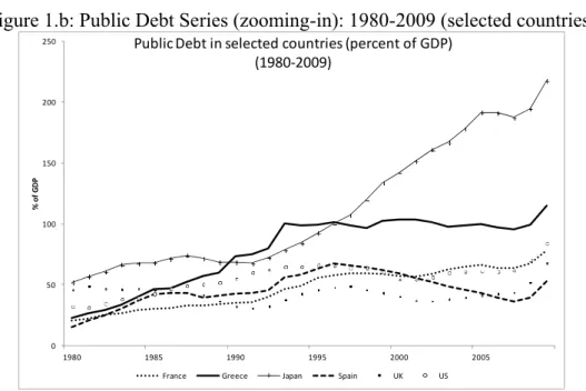
the public paths of selected countries, as depicted in Figure 1a. It is clear from this chart that

government debt-to-GDP ratios peaked around the two World Wars in the 20th century and

then again after the 1970s till the end of the 1990s – with the exception of Japan where debt

kept on rising. Government debt restarted an increasing trend with the 2008 economic crisis

and the continuous worsening state of public finances in most advanced and emerging

economies (Figure 1b).

Figure 1.a: Public Debt Series: 1880-2009 (selected countries)

0 50 100 150 200 250 300

1880 1890 1900 1910 1920 1930 1940 1950 1960 1970 1980 1990 2000

% o

f

G

D

P

Public Debt in selected countries (percent of GDP) (1880‐2009)

France Greece Japan Spain UK US

Source: Abbas et al. (2010).

Figure 1.b: Public Debt Series (zooming-in): 1980-2009 (selected countries)

0 50 100 150 200 250

1980 1985 1990 1995 2000 2005

% o

f

G

D

P

Public Debt in selected countries (percent of GDP)

(1980‐2009)

France Greece Japan Spain UK US

For instance, government debt increased in Italy from an average of 51.8% of GDP in the

1970s to an average of 112.3% in the 2000s (Table 1). Nevertheless, Italy reduced its debt

level in 3.8 percentage points (pp) relative to the average figure in 1880s. On the other hand,

Japan’s debt increased by about 143.5 pp between the 1880s and the 2000s, followed by

Belgium, the US, Sweden and Argentina (see last column in Table 1). In the case of Greece,

Italy and Japan government debt has surpassed 100% of GDP, an average value that was kept

during the 2000s. In the cases of Belgium and Italy, their high debt service payments induced

substantial budget deficits despite primary surpluses. A reversal of that general trend is

noticeable only at the end of the 1990s, as several “more indebted” European countries tried

to fulfil or at least come closer to the Maastricht criteria (much of that effort was afterwards

reversed, notably in the context of the 2008-2009 economic and financial crisis). All in all, the

main conclusion is that the burden of government debt has increased over time in almost

every country under scrutiny.

[Table 1]

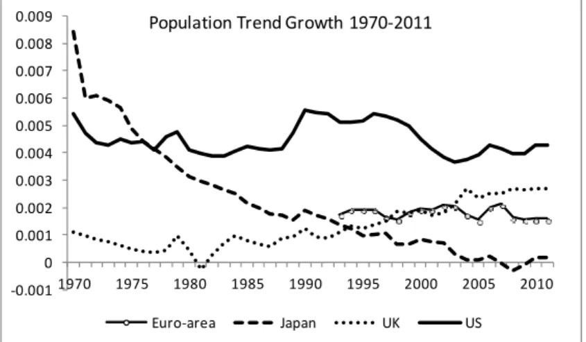
It is nevertheless important to be aware that the main driver for (potential) lack of fiscal

sustainability in the near future (particularly in the context of the government debt increase

following the last economic and financial crisis) will be population growth (see Figure 2a. and

2.b), combined with generous pay-as-you-go social security systems in advanced economies.

Figure 2.a: Trend Growth of Population: 1970-2011 (selected countries)

‐0.001 0 0.001 0.002 0.003 0.004 0.005 0.006 0.007 0.008 0.009

1970 1975 1980 1985 1990 1995 2000 2005 2010

Population Trend Growth 1970‐2011

Euro‐area Japan UK US

Figure 2.b: Forecasting Population (level) with STM: 2000-2016 (selected countries)

(a)

2.48 2.49 2.5 2.51 2.52 2.53 2.54

2000 2005 2010 2015

Forecasting Euro‐area population (level)

(b)

2.1 2.105 2.11 2.115 2.12

2000 2005 2010 2015

Forecasting Japan population (level)

(c)

1.76 1.77 1.78 1.79 1.8 1.81 1.82

2000 2005 2010 2015

Forecasting UK population (level)

(d)

2.44 2.45 2.46 2.47 2.48 2.49 2.5 2.51

2000 2005 2010 2015

Forecasting US population (level)

Note: Authors’ calculations based on fitted univariate STM applied to the log of total population and recursively forecasted using the Kalman filter up to 5 years ahead and using information from 2000 till 2011.

Since this population shift towards older societies is an entirely new phenomenon, it

cannot be considered in terms of the econometric analysis based exclusively on past data,

notably regarding explicit liabilities. Indeed, implicit pension liabilities will impinge on future

borrowing requirements, and can carry additional sustainability issues. Figure 2.b suggests

that population growth will put extra pressure on Euro-area, UK and US budgets (given

computed projections), less so in the case of Japan (also attested by declining, and close to

zero, population trend growth).

Country Unit Root Analysis

Before presenting the results of unit roots tests, it should be mentioned that the fact that

our series are in ratio to GDP does not rule them out being integrated processes (see, Ahmed

and Yoo, 1989). Hence, we focus on fiscal policy sustainability for each of the 19 countries

by means of several unit root tests in an attempt to validate the sufficient sustainability

condition using the stock of government debt. Table 2 shows the stationarity tests results for

the first difference of the debt ratio for the period 1880-2009.

The results for the ADF and PP test (considering both a constant and a time trend) allow

the rejection of the null of a unit root in all countries but Japan. Therefore, the series of the

first difference of government debt might be I(0) over the very long-run and the solvency

condition would be satisfied in those cases since non-stationarity can be rejected, and,

therefore, longer-run fiscal sustainability cannot. The Ng and Perron (2001) tests give us

similar conclusions (apart from the case of Spain). One should also note that contrary to

several other studies on fiscal sustainability, which have to rely on a small number of

observations, accuracy problems of unit-root tests with small samples do not apply in our

case.

The previous set of results assumes that there is no structural break in the government

debt series. However, this might not be the case in some countries – for example, in periods of

war or important economic downturns. In the presence of structural changes in the trend

function, ADF and PP tests that do not take into account the break in the series have low

power, and are biased toward the non-rejection of a unit root. Therefore, in Table 2 we also

report the identified structural breaks, with many occurrences taking place in the 1st half of the

21st century. Interestingly, we also see structural breaks in European countries when the

so-called expansionary fiscal consolidations took place, notably in Sweden, in 1991 and in 1996,

and in Denmark in the periods 1982-1983.16

Consequently, the longer historical time span proves to be crucial to assess fiscal

sustainability. Indeed, while most existing empirical analysis conclude for absence of fiscal

sustainability for many countries, such studies usually have a much more limited data time

span, starting essentially in the 1970s.

Cyclical Behaviour

In order to evaluate the possibility of the presence of a cyclical component in the

government debt series, some descriptive statistics (not shown) such as the correlogram and

the power spectrum can provide useful information. If sometimes the correlogram shows only

small individual autocorrelations, not providing enough strong evidence of the presence of

cyclical movement in the series (despite that some cycle evidence may be buried with noise),

then a much clearer message emerges from the examination of the spectrum.

Based on the information gathered by conducting unit root tests and the descriptive

statistics employed to evaluate the presence of cyclical movements in the debt series, a likely

_____________________________

16

specification for the trend and the cyclical components of a structural time series model for

the different data can be estimated. Table 3 shows main diagnostic and goodness-of-fit

statistics for a basic structural model.17 All these models assume the presence of a trend, one

cycle and an irregular component.18

[Table 3]

The diagnostics are generally satisfactory and the estimation of alternative models, such

as a linear trend model, a smooth trend model or even a random walk with drift, yielded

poorer statistics relative to the selected Basic Structural Model.

The estimated variances for the hyper-parameters together with the period (in years) of the

cycle are presented in Table 4.

[Table 4]

A first comment goes to the period of the cycle which varies between 7.03 years for

Greece and 23.71 years for Portugal. Secondly, none of the models show a q-ratio19

associated with the irregular component exactly equal to 1 (with the exception of Greece),

meaning that all the variation in those time series is explained by the trend, cycles and

interventions (whenever present). Ideally we would like 2 ε

σ to be as small as possible, and let

the other components explain most of the model’s variation.

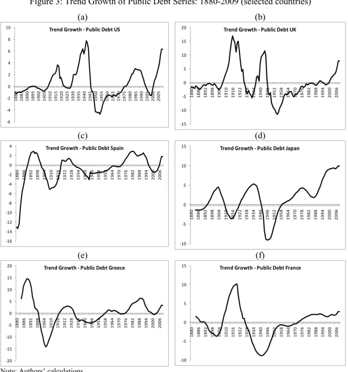
Given this model for each country, the graphs of the trend growth resulting from the STM

for the government debt series are displayed in Figure 3 for a subset of countries (for reasons

of parsimony other graphs are available upon request).

Increases in government debt are naturally associated with times of increased military

expenditure, hence notably during the two World Wars. A spike is also visible around the

1970s with the oil price shocks and government’s efforts to keep their energy supplies even at

increasing costs. More recently, since the early 2000s both the UK and the US to a greater

extent and Spain and Greece to a lesser extent experienced a sudden increase in their debt

trend growth rates; less so in the case of France, whereas in Japan such phenomenon began

_____________________________

17

Diagnostic checking tests are conducted by computing the Box-Ljung Q(n) statistic for serial correlation and a simple test for heteroscedasticity H(n,m). The Prediction Error Variance (PEV), the coefficient of determination (Rd^2) and the information criteria (Akaike Information Criteria, AIC; and Bayesian Information Criteria, BIC) proved goodness-of-fit measures. Table 2 also presents information related to the Log-Likelihood.

18

Other models have been estimated but yield less satisfactory diagnostics, based on information criteria assessment. These are available upon request and consisted of: i) a statistical specification that assumes that the trend component follows a random walk with drift, with a deterministic slope; ii) a second which introduces a somewhat smoother trend with a deterministic level and a stochastic slope; iii) finally, we have estimated local linear trend model, which stipulates the level and slope to be stochastic.

19

back in the early 1990s following their economic (asset price) bubble and financial crisis from

1986-1991 which continued up to the current period.

Figure 3: Trend Growth of Public Debt Series: 1880-2009 (selected countries)

(a) ‐6 ‐4 ‐2 0 2 4 6 8 10 18 80 18 85 18 90 18 95 19 00 19 05 19 10 19 15 19 20 19 25 19 30 19 35 19 40 19 45 19 50 19 55 19 60 19 65 19 70 19 75 19 80 19 85 19 90 19 95 20 00 20 05

Trend Growth ‐Public Debt US

(b) ‐15 ‐10 ‐5 0 5 10 15 20

1880 1886 1892 1898 1904 1910 1916 1922 1928 1934 1940 1946 1952 1958 1964 1970 1976 1982 1988 1994 2000 2006

Trend Growth ‐Public Debt UK

(c) ‐16 ‐14 ‐12 ‐10 ‐8 ‐6 ‐4 ‐2 0 2 4 1 880 1 886 1 892 1 898 1 904 1 910 1 916 1 922 1 928 1 934 1 940 1 946 1 952 1 958 1 964 1 970 1 976 1 982 1 988 1 994 2 000 2 006

Trend Growth ‐Public Debt Spain

(d) ‐10 ‐5 0 5 10 15 18 80 18 86 18 92 18 98 19 04 19 10 19 16 19 22 19 28 19 34 19 40 19 46 19 52 19 58 19 64 19 70 19 76 19 82 19 88 19 94 20 00 20 06

Trend Growth ‐Public Debt Japan

(e) ‐20 ‐15 ‐10 ‐5 0 5 10 15 20

1880 1886 1892 1898 1904 1910 1916 1922 1928 1934 1940 1946 1952 1958 1964 1970 1976 1982 1988 1994 2000 2006

Trend Growth ‐Public Debt Greece

(f) ‐10 ‐5 0 5 10 15 188 0 188 6 189 2 189 8 190 4 191 0 191 6 192 2 192 8 193 4 194 0 194 6 195 2 195 8 196 4 197 0 197 6 198 2 198 8 199 4 200 0 200 6

Trend Growth ‐Public Debt France

Note: Authors’ calculations.

The government debt series depicted above are characterized by cycles which show great

volatility during the first half of the 20th century and then again around the period associated

with the oil price shocks. Particularly over the 1950s and 1960s (the so-called “Golden Age”

of economic growth), and then after the entry in the EU of many European countries, these

cyclical variations are much reduced. Given the important cyclical variation of the short

4, which presents the Kernel density estimates20 of the (STM) cyclical deviation of

government debt over the full span of the period 1880-2009 and the sub-periods 1910-1973,

1973-1999, 1926-1973, 1913-1945, 1945-2009 (according to Angus Maddison's growth

phases split). It is clear that any period is more stable than the inter-war years.

Figure 4: Short cycles: Kernel Density Estimates of Public Debt Series: 1880-2009 (selected countries) (a) 0 0.2 0.4 0.6 0.8 1 1.2 1.4

‐10 5 0 5 10

US

1880‐2009 1880‐1913 1945‐2009 1913‐1945 1970‐2009

(b) 0 0.02 0.04 0.06 0.08 0.1 0.12

‐10 5 0 5 10

UK

1880‐2009 1880‐1913 1945‐2009 1913‐1945 1970‐2009

(c) 0 0.2 0.4 0.6 0.8 1 1.2 1.4 1.6 1.8 2

‐10 5 0 5 10

Spain

1880‐2009 1880‐1913 1945‐2009 1913‐1945 1970‐2009

(d) 0 0.02 0.04 0.06 0.08 0.1 0.12 0.14 0.16

‐10 5 0 5 10

Japan

1880‐2009 1880‐1913 1945‐2009 1913‐1945 1970‐2009

(e) 0 0.1 0.2 0.3 0.4 0.5 0.6

‐10 5 0 5 10

Greece

1880‐2009 1880‐1913 1945‐2009 1913‐1945 1970‐2009

(f) 0 0.02 0.04 0.06 0.08 0.1 0.12 0.14

‐10 5 0 5 10

France

1880‐2009 1880‐1913 1945‐2009 1913‐1945 1970‐2009

Note: Authors’ calculations.

_____________________________

20

Panel Unit Root Analysis

A panel analysis can also be considered to take advantage of the increased number of

observations. In addition, the nature of the interactions and dependencies that generally exist,

over time and across the individual units in the panel, can then also be taken into account. For

instance, and as already mentioned, cross-country dependence can also be envisaged notably

via some level of integration of financial markets, while spillover effects in government bond

markets and interest rates co-movements are to be expected.

Therefore, we take advantage of the long cross-section of time series available and

conduct first and second general panel unit root tests. The results of such analysis are

displayed in Tables 5a and 5b. The conclusions go in the same direction as the ones reached

for the individual country unit-root tests, that is, for the first-differenced debt at lags 0-2 both

first and second generation panel unit root tests reject the null that all country series contain a

nonstationary process. Therefore, is not possible to reject the hypothesis of sustainability of

public finances in the context of this panel sample.

[Tables 5a-5b]

“Debt-trackers”

Finally, as an additional illustration, and following Matheson’s (2011)21 approach, we

constructed the so-called “debt-trackers” using our long series for the same selection of

countries. The heat map in Figure 5 displays information about government debt for selected

countries: the US, UK, Japan, Spain, France and Greece. The trends used in the heat map are

computed by means of univariate STM estimated using the Kalman filter. The colors are

based on the behavior of the smoothed series relative to trend: a yellow color indicates growth

below trend and moderating; red and pink indicate growth of debt above trend at increasing

and decreasing rates, respectively; the darkest shade of green represents contraction of debt,

with the lightest green indicating a debt growth below trend and moderating.

Therefore, the heat map in Figure 5 clearly shows the implications of the global

financial crisis for government debt in 2008 and 2009. The effects of the crisis were seen

_____________________________

21

across the represented countries (to a less extent in Japan, which had a very high debt level to

start with).

[Figure 5]

5. Conclusion

In this paper we have revisisited the issue of fiscal policy sustainability in a set of 19

countries by taking a longer-run secular perspective covering the period 1880-2009. In our

empirical assessment we also performed a systematic analysis of the stationarity properties of

the first-differenced level of government debt.

Via a systematic analysis of the stationarity properties of the first-differenced level of

government debt, we are able to conclude that the solvency condition would be satisfied in

mostly all cases since non-stationarity can be rejected, and, therefore, longer-run fiscal

sustainability cannot (Japan and Spain can be exceptions). In addtion, the implications of the

global financial crisis for government debt in 2008 and 2009 are also picked up in the

analysis.

Interestingly, the results of our paper may be considered as more “pleasant” over the very

long run from a policy-maker’s point of view, than some previously existing fiscal

sustainability analysis where the time spans were much shorter. Still, and even if that may be

the case for the existing explicit government liabilities, one needs to bear in mind that any

policy measures in that area are probably more than needed to tackle the burden of incoming

implicit liabilities in most countries.

On the other hand, it is also not possible to reject the hypothesis of sustainability of public

finances in the context of this longer time span panel sample, which is nevertheless in line

References

1. Abbas, A., Belhocine, N., ElGanainy, A., Horton, M. (2010), “A Historical Public Debt

Database”, IMF Working Paper No. 10/245.

2. Afonso, A. (2005), “Fiscal Sustainability: the Unpleasant European Case”, FinanzArchiv,

61 (1), 19-44.

3. Afonso, A. (2008), “Ricardian Fiscal Regimes in the European Union”, Empirica, 35 (3),

313–334.

4. Afonso, A. (2010), “Expansionary fiscal consolidations in Europe: new evidence”,

Applied Economics Letters, 17, 105-109.

5. Afonso, A. and Rault, C. (2010), “What do we really know about fiscal sustainability in

the EU? A panel data diagnostic,” Review of World Economics, 145, (4), 731-755.

6. Ahmed, S. and Rogers J. H. (1995), “Government budget deficits and trade deficits Are

present value constraints satisfied in long-term data”, Journal of Monetary Economics

36(2), 351-374.

7. Ahmed, S. and Yoo, B. (1989), “Fiscal trends and real business cycles”, Working paper,

Pennsylvania State University, University Park, PA.

8. Andrews, D.W. K., and Ploberger, W. (1994), “Optimal Tests When a Nuisance

Parameter Is Present Only Under the Alternative”, Econometrica, 62, 1383-1414.

9. Arghyrou, Michael G. and Kul B. Luintel (2007), “Government Solvency: Revisiting

Some EMU Countries”, Journal of Macroeconomics 29, 387-410.

10.Bergman, M. (2001), “Testing Government Solvency and the No Ponzi Game Condition”,

Applied Economics Letters, 8(1), 27-29.

11.Bohn, H. (1991), “The Sustainability of Budget Deficits with Lump-Sum and with

Income-Based Taxation”, Journal of Money, Credit, and Banking 23 (3), Part 2: 581-604.

12.Bohn, H. (1998), “The Behavior of U.S. Public Debt and Deficits”, Quarterly Journal of

Economics 113, 949-963.

13.Bohn, H. (2007), “Are Stationarity and Cointegration Restrictions Really Necessary for

the Intertemporal Budget Constraint?” Journal of Monetary Economics, 54(7), 1837-1847.

14.Bravo, A. B. S., Silvestre, A. L. (2002), “Intertemporal Sustainability of Fiscal Policies:

Some Tests for European Countries”, European Journal of Political Economy, 18, 517–

528.

15.Buiter, W.H. (2002), “The Fiscal Theory of the Price Level: A Critique”, Economic

16.Chalk, N. and Hemming, R. (2000), “Assessing fiscal sustainability in theory and

practice”, (IMF Working Paper No. 00/81). International Monetary Fund.

17.Clemente, J., Montañés, A., and Reyes, M. (1998), “Testing for a unit root in variables

with a double change in the mean”, Economics Letters, 59, 175-182.

18.Cogley, T., and Nason, J. M. (1995), "Effects of the Hodrick-Prescott filter on trend and

difference stationary time series: Implications for business cycle research", Journal of

Economic Dynamics and Control, 19, 253-278.

19.Cuddington, J. (1997), “Analysing the Sustainability of Fiscal Deficits in Developing

Countries”, Policy Research Working Paper nº 1784, World Bank.

20.Feve, P., and Henin, P.Y. (2000), “Assessing Effective Sustainability of Fiscal Policy

within the G-7”, Oxford Bulletin of Economics and Statistics, 62, 175.

21.Hakkio, C.S., and Rush, M. (1991), “Is the Budget Deficit “Too Large”?” Economic

Inquiry 29, 429-445.

22.Hamilton, J.D., and Flavin, M.A. (1986), “On the Limitations of Government Borrowing:

A Framework for Empirical Testing”, American Economic Review 76, 808-819.

23.Harvey, A. (1989), "Forecasting, Structural time series and the Kalman Filter", Cambridge

UK, Cambridge University Press.

24.Harvey, A. C. (1997), "Trends, cycles and autoregressions", Economic Journal, 107,

192-201.

25.Harvey, A. C. (2001), "Trends, cycles and convergence", Proceedings of Fifth Annual

Conference of Bank of Chile.

26.Harvey, A. C. and N. Shephard (1993), Structural time series models, in Handbook of

Statistics, 11, edited by G. S. Maddala, C. R. Rao and H. D. Vinod, Elsevier Science

Publishers B.V.

27.Harvey, A. C., and Jaeger, A. (1993), "Detrending, stylized facts and the business cycle",

Journal of Applied Econometrics, 8, 231-247.

28.Harvey, A.C., Scott, A., (1994). “Seasonality in dynamic regression models.” Economic

Journal (104), pp 1324–1345.

29.Hatemi-J A. (2002), “Fiscal Policy in Sweden: Effects of EMU Criteria Convergence”,

Economic Modelling, 19 (1).

30.Hénin, P. (1997), “Soutenabilité des déficits et ajustements budgétaires”, Révue

Économique 48 (3), 371-395.

31.Im, K. S., Pesaran, M. H. and Shin, Y. (2003), “Testing for unit roots in heterogeneous

32.Joines, D. (1991), “How large a federal deficit can we sustain?”, Contemporary Policy

Issues 9 (3), 1-11.

33.Jong, P. and Penzer, J. (1998) Diagnosing shocks in time series. Journal of the American

Statistical Association. 93, 796-806.

34.Keynes, J. M. (1923), “A Tract on Monetary Reform”, (London & Cambridge, Macmillan

& Cambridge University Press, 1971–82).

35.MacDonald, R. (1992), “Some Tests of the Government Intertemporal Budget Constraint

Using U.S. Data”, Applied Economics 24(12): 1287-92.

36.Maddala, G. S., and Wu, S. (1999). A Comparative Study of Unit Root Tests with Panel

Data and New Simple Test", Oxford Bulletin of Economics and Statistics, 61, 631-652

37.Makrydakis S., Tzavalis E. and Balfoussias A. (1999), “Policy regime changes and the

long-run sustainability of fiscal policy: an application to Greece”, Economic Modelling

16, 71-86.

38.Martin, G.M. (2000), “U.S. Deficit Sustainability: A New Approach Based on Multiple

Endogenous Breaks”, Journal of Applied Econometrics, 15(1), pp. 83–105.

39.Matheson, T. (2011). “New Indicators for Tracking Growth in Real-Time”, IMF WP No.

1143.

40.McCallum, B. (1984), “Are Bond-Financed Deficits Inflationary? A Ricardian Analysis”,

Journal of Political Economy 92, 123-135.

41.Mendoza, E.G., and J.D. Ostry (2008), “International Evidence on Fiscal Solvency: Is

Fiscal Policy ‘Responsible’?” Journal of Monetary Economics, 55(6) 1081–93.

42.Ng, S., and P. Perron (2001), “Lag Length Selection and the Construction of Unit Root

Tests with Good Size and Power,” Econometrica, 69, 1519-1554.

43.O'Connell, P. (1998), “The Overvaluation of Purchasing Power Parity”, Journal of

International Economics, 44, 1-19.

44.Perron, P. (1989), “The Great Crash, the Oil Price Shock, and the Unit Root Hypothesis.”

Econometrica 57, 1361-1401.

45.Perron, P. and Yabu, T. (2009), “Testing for Shifts in Trend with an Integrated or

Stationary Noise Component”, Journal of Business and Economics Statistics, 27, 369-396.

46.Pesaran, M.H., (2007), “A simple panel unit root test in the presence of cross section

dependence”, Journal of Applied Econometrics, 22, 265-312.

47.Quintos, C.E. (1995), “Sustainability of the Deficit Process with Structural Shifts”,

48.Roy, A., and Fuller, W.A. (2001), “Estimation for Autoregressive Processes With a Root

Near One,” Journal of Business and Economic Statistics, 19, 482-493.

49.Trehan, B., and Walsh, C. (1991), “Testing Intertemporal Budget Constraints: Theory and

Applications to U.S. Federal Budget and Current Account Deficits”, Journal of Money,

Credit and Banking 23, 210-223.

50.Vogelsang, T. (2001), “Testing for a Shift in Trend When Serial Correlation is of

Unknown Form,” Unpublished Manuscript, Department of Economics, Cornell

University.

51.Vogelsang, T. and P. Perron (1998), “Additional Tests for a Unit Root Allowing for a

Break in the Trend Function at an Unknown Time”, International Economic Review

39(4), 1073-1100.

52.Zivot, E. and D. W. K. Andrews (1992), “Further Evidence on the Great Crash, the

Oil-Price Shock and the Unit Root Hypothesis”, Journal of Business and Economic Statistics

Figure 5: Debt-Trackers (selected countries) 1881-2009

1881 1882 1883 1884 1885 1886 1887 1888 1889 1890 1891 1892 1893 1894 1895 1896 1897 1898 1899 1900 1901 1902 1903 1904 1905 1906 1907 1908 1909 1910 1911 1912 1913 1914 1915 1916 1917 1918 1919 1920 1921 1922 1923 1924

US UK Japan Spain France Greece

1925 1926 1927 1928 1929 1930 1931 1932 1933 1934 1935 1936 1937 1938 1939 1940 1941 1942 1943 1944 1945 1946 1947 1948 1949 1950 1951 1952 1953 1954 1955 1956 1957 1958 1959 1960 1961 1962 1963 1964 1965 1966 1967

US UK Japan Spain France Greece 196 8 196 9 197 0 197 1 197 2 197 2 197 3 197 4 197 5 197 6 197 7 197 8 197 9 198 0 198 1 198 2 198 3 198 4 198 5 198 6 198 7 198 8 198 9 199 0 199 1 199 2 199 3 199 4 199 5 199 6 199 7 199 8 199 9 200 0 200 1 200 2 200 3 200 4 200 5 200 6 200 7 200 8 200 9 US UK Japan Spain France Greece

contraction at an increasing rate contraction at a moderating rate growth below trend and moderating growth below trend and rising

growth above trend and moderating

growth above trend and rising

TABLE 1. Public Debt (% of GDP), decade averages: 1880-2009

country 1880s 1890s 1900s 1910s 1920s 1930s 1940s 1950s 1960s 1970s 1980s 1990s 2000s Diff. (p.p.) ranking

Argentina 50.8 87.9 44.0 27.3 43.7 51.3 29.4 15.3 13.8 46.1 39.5 83.9 33.1

growth rel. prev. 23.8 -30.1 -20.7 7.0 -24.1 -28.6 -4.4 52.5 -6.8 32.8 5

Austria 78.5 85.1 71.6 64.1 19.9 32.3 27.9 14.0 15.9 21.5 47.0 63.0 64.8 -13.7 12

growth rel. prev. 3.5 -7.5 -4.8 -50.8 21.0 -6.4 -29.8 5.4 13.1 33.9 12.8 1.2

Belgium 40.0 47.7 48.3 45.6 107.6 81.9 123.3 66.9 58.4 44.8 92.7 124.1 97.6 57.6 2

growth rel. prev. 7.7 0.5 -2.4 37.2 -11.8 17.8 -26.6 -5.9 -11.5 31.6 12.7 -10.5

Brazil 104.6 70.8 54.3 36.9 25.0 32.5 25.2 9.3 31.1 53.6 60.4 70.2 -34.4 14

growth rel. prev. -16.9 -11.5 -16.8 -16.9 11.4 -11.1 -43.4 23.6 5.2 6.5

Denmark 23.0 18.5 16.3 14.6 19.6 20.1 10.9 28.0 16.4 14.8 54.2 65.1 50.8 27.8 8

growth rel. prev. -9.4 -5.6 -4.8 12.9 1.1 -26.4 40.8 -23.3 -4.4 56.4 8.0 -10.8

France 105.2 102.8 87.7 90.9 179.6 159.2 42.2 33.4 20.0 17.4 29.2 50.4 63.5 -41.6 16

growth rel. prev. -1.0 -6.9 1.6 29.6 -5.2 -57.7 -10.2 -22.1 -6.0 22.4 23.7 10.0

Germany 35.3 42.8 39.7 39.9 10.2 20.3 17.8 18.7 19.4 23.3 39.2 52.1 64.5 29.2 7

growth rel. prev. 8.4 -3.3 0.3 -59.3 30.0 -5.9 2.3 1.4 7.9 22.7 12.3 9.3

Greece 90.3 182.4 162.9 84.2 84.9 85.2 16.9 19.4 23.7 44.5 93.6 101.3 11.0 9

growth rel. prev. 30.6 -4.9 -28.7 0.4 0.1 5.9 8.8 27.3 32.3 3.4

Italy 111.4 116.7 97.9 94.6 121.3 82.8 61.7 32.1 31.8 51.8 77.9 112.3 107.6 -3.8 10

growth rel. prev. 2.0 -7.7 -1.5 10.8 -16.6 -12.8 -28.4 -0.5 21.2 17.7 15.9 -1.9

Japan 30.7 23.3 48.0 45.9 35.0 62.8 75.0 11.0 7.3 28.3 66.1 97.1 174.2 143.5 1

growth rel. prev. -12.0 31.4 -2.0 -11.7 25.4 7.7 -83.5 -17.4 58.5 36.9 16.7 25.4

Netherlands 89.2 90.1 67.7 50.6 49.1 63.5 218.0 76.7 71.1 56.4 79.8 86.3 54.2 -35.0 15

growth rel. prev. 0.4 -12.4 -12.7 -1.3 11.2 53.6 -45.4 -3.3 -10.1 15.1 3.4 -20.2

New Zealand 108.6 126.5 115.1 116.2 149.0 181.5 134.1 82.7 62.1 47.9 61.6 50.8 24.4 -84.3 19

growth rel. prev. 6.6 -4.1 0.4 10.8 8.6 -13.1 -21.0 -12.5 -11.2 10.9 -8.4 -31.9

Norway 16.2 20.0 27.1 17.8 30.2 33.8 42.3 26.7 25.1 30.2 39.3 40.7 47.3 31.1 6

growth rel. prev. 9.1 13.2 -18.2 22.8 5.0 9.7 -20.0 -2.7 8.1 11.4 1.6 6.5

Portugal 84.2 99.9 78.0 73.2 31.3 24.3 38.7 30.7 50.7 56.5 60.1 -24.1 13

growth rel. prev. 7.5 -10.7 -2.8 -11.1 20.3 -10.1 21.8 4.7 2.6

Russia 78.7 71.8 57.9 49.8 72.7 30.9 -47.8 18

growth rel. prev. -4.0 -9.3 -6.5 -37.2

Spain 94.9 92.4 107.9 62.5 57.1 62.6 47.2 23.6 15.6 12.9 34.5 57.1 48.7 -46.2 17

growth rel. prev. -1.1 6.7 -23.7 -4.0 4.1 -12.3 -30.2 -18.0 -8.2 42.8 21.9 -6.9

Sweden 18.1 17.0 15.8 15.6 18.9 23.5 39.9 30.4 28.9 31.3 60.1 73.2 52.8 34.6 4

growth rel. prev. -3.0 -2.9 -0.6 8.3 9.4 23.0 -11.8 -2.2 3.4 28.4 8.5 -14.2

UK 56.7 41.9 36.9 68.5 174.8 169.0 202.5 157.7 97.5 54.5 44.0 41.1 44.4 -12.4 11

growth rel. prev. -13.1 -5.5 26.9 40.7 -1.5 7.9 -10.9 -20.9 -25.3 -9.3 -3.0 3.3

US 12.5 7.2 4.6 9.9 23.3 37.3 84.4 66.9 45.5 34.1 43.3 62.4 62.7 50.2 3

growth rel. prev. -24.1 -18.9 33.0 37.2 20.3 35.5 -10.1 -16.7 -12.5 10.4 15.9 0.1

TABLE 2. Unit Root Tests and Structural Breaks: First-Differenced Public Debt 1880-2009

Countries

ADF PP NP

ZA VP(AO) VP(IO) CMR(AO) CMR(IO) PY2009

MZa MZt MSB MPT

(1) (2) (3) (4) (5) (6) (7) (8) (9) (10) (11) (12)

Argentina -5.29*** -9.35*** -74.29*** -6.09*** 0.08*** 0.32*** 1906*** 2000** 2000** 1999, 2002 1892, 2000** 1961***

Austria -6.65*** -6.65*** -34.06*** -4.11*** 0.12*** 0.75*** 1926*** 1912 1913 1912, 1922 1913, 1923** 1912***

Belgium -6.00*** -5.73*** -17.05*** -2.87*** 0.16** 1.60** 1944*** 1939** 1940** 1944, 1946 1938, 1942** 1962***

Brazil -10.48*** -11.17*** -13.21** -2.57** 0.19*** 1.85*** 1990*** 1986 1987** 1891, 1986 1892, 1987** 1946*

Denmark -5.30*** -5.13*** -31.84*** -3.98*** 0.12*** 0.77*** 1977*** 1980 1983** 1978, 1982 1975, 1984** 1959***

France -13.02*** -12.17*** -50.17*** -4.94*** 0.09*** 0.65*** 1923*** 1919 1920** 1919, 1947 1920, 1948 1925***

Germany -7.20*** -7.26*** -20.51*** -3.15*** 0.15*** 1.37*** 1926*** 1923 1924** 1912, 1923 1913, 1924** 1956***

Greece -4.77*** -9.22*** -11.22** -2.25** 0.20*** 2.61*** 1901*** 1892 1893** 1892, 1909 1895, 1912** 1920***

Italy -8.38*** -8.35*** -7.47* -1.92* 0.25* 3.29* 1921*** 1917** 1918** 1917, 1944 1918, 1945** 1944***

Japan 0.09 -2.75* -16.49*** -2.67*** 0.16** 2.19** 1945*** 1942** 1943** 1942, 1948 1943, 1948** 1945***

Netherlands -6.39*** -6.40*** -45.28*** -4.78*** 0.10*** 0.56*** 1947*** 1944 1945 1944, 1958** 1945, 1959** 1930***

New Zealand -7.49*** -6.27*** -83.71*** -6.45*** 0.07*** 0.30*** 1934*** 1935 1931** 1935, 1939 1931, 1939 1949*

Norway -7.66*** -7.37*** -49.91*** -4.98*** 0.09*** 0.50*** 1948*** 1948** 1949** 1991, 1999 1992, 1998** 1987***

Portugal -7.06*** -7.06*** -36.45*** -4.19*** 0.11*** 0.88*** 1915*** 1911** 1912 1900, 1911 1890, 1912** 1911***

Russian Federation -4.82*** -4.89*** -13.04** -2.55** 0.19*** 1.87** 1913*** 1990** 1991** 1990, 1996 1991, 1998** 1925***

Spain -7.74*** -7.67*** -0.27 -0.12 0.47 16.97 1900*** 1943** 1944** 1912, 1943 1913, 1944** 1964***

Sweden -4.51*** -4.65*** -29.45*** -3.79*** 0.12*** 0.95*** 1977*** 1990** 1991** 1978, 1996** 1989, 1996** 1954***

United Kingdom -5.18*** -5.24*** -37.95*** -4.28*** 0.11*** 0.85*** 1947*** 1943** 1945** 1942, 1944 1939, 1945 1917***

United States -6.33*** -4.98*** -72.10*** -5.87*** 0.08*** 0.61*** 1947*** 1943 1944** 1939, 1943 1941, 1944** 1941***

Note: ADF critical values: -4.028, -3.445, -3.145 for 1, 5 and 10% levels respectively. For the Ng-Perron test (NP), none of the test statistics are significant at the usual levels. The critical values are taken from Ng and Perron (2001), table 1 and the autoregressive truncation lag (zero) has been selected using the modified AIC. The ZA test statistic reported is the minimum Dickey-Fuller statistic calculated across all possible breaks in the series, when both a break in the intercept and the time trend is allowed for. The year in parenthesis denotes the year when this minimum DF statistic is obtained. The 1% critical value is -5.57 and the 5% critical value is -5.08. As for the VP test, “AO” means addictive outlier and “IO” means innovational outlier and critical values are taken from Perron and Vogelsang (1992), in particular, -3.56 (AO) and -4.27 (IO) for 5% level. As for CMR the 5% critical value is -5.49 (both AO and IO), also taken from Perron and Vogelsang (1992). In column 10 we run the Perron-Yabu (PY) unit root test. For the structural-break type tests only dates are presented and when applicable, a statistically significant symbol is added. The null in the non-break type tests is of unit root. The null in the non-break-type tests is of unit root against the non-break stationary alternative hypothesis.

TABLE 3. Structural Time Series Models: Diagnostic and Goodness-of-fit statistics, Public Debt 1880-2009

Basic Structural Model Log-Li. P.E.V. H(h) Q(p,q) Rd^2 AIC BIC

Argentina -250.925 212.744 4.451 4.991 0.084 5.407 5.475 Austria -124.965 9.519 0.479 14.743 0.623 2.299 2.365 Belgium -240.111 74.728 0.907 39.514 0.774 4.36 4.426 Brazil -212.365 104.901 2.201 11.802 0.122 4.700 4.768 Denmark -108.627 7.160 8.321 12.979 0.558 2.016 2.083 France -241.475 108.976 0.031 15.016 0.708 4.738 4.806

Germany -92.118 5.394 0.607 9.0637 0.684 1.732 1.800 Greece -239.807 152.784 0.091 24.729 0.257 5.076 5.142

Italy -267.251 71.390 0.124 24.548 0.075 4.315 4.383 Japan -316.344 170.517 0.476 21.820 0.371 5.185 5.254 Netherlands -174.364 24.073 1.004 16.062 0.934 3.228 3.296 New Zealand -270.969 78.792 0.267 45.993 0.134 4.414 4.482 Norway -155.037 14.621 5.319 15.314 0.387 2.730 2.797 Portugal -136.207 18.390 0.407 22.023 0.533 2.958 3.024 Russian Federation -99.498 61.374 2.404 17.903 0.679 4.165 4.232 Spain -231.959 54.259 0.153 6.3130 0.238 4.039 4.106 Sweden -122.354 9.176 15.77 20.662 0.519 2.262 2.329 United Kingdom -271.397 68.033 0.222 22.660 0.348 4.266 4.332 United States -195.735 20.820 0.577 20.936 0.238 3.082 3.148

TABLE 4. Structural Time Series Models: Estimated variances of disturbances, Public Debt 1880-2009

country 2

η σ 2 ζ σ 2 1 c σ 2 ε

σ Period 1

Argentina 43.45 0.00 94.05 25.23 19.87 (0.46) (0.00) (1.00) (0.26) Austria 5.85 0.60 0.26 0.00 7.15 (1.00) (0.10) (0.04) (0.00) Belgium 0.00 27.79 10.12 2.23 9.65 (0.00) (1.00) (0.36) (0.08) Brazil 0.00 0.08 84.37 0.00 19.43 (0.00) (0.00) (1.00) (0.00) Denmark 3.38 0.81 0.66 0.00 15.13 (1.00) (0.24) (0.19) (0.00)

France 0.00 4.12 26.18 18.06 15.16 (0.00) (0.16) (1.00) (0.69)

Germany 3.12 0.46 0.14 0.00 7.46 (1.00) (0.15) (0.04) (0.00)

Greece 16.53 6.99 0.74 49.33 7.03 (0.34) (0.14) (0.02) (1.00)

Italy 58.00 0.06 4.10 0.00 11.09 (1.00) (0.00) (0.07) (0.00)

Japan 0.00 4.60 84.30 0.00 11.60 (0.00) (0.05) (1.00) (0.00)

Netherlands 4.86 15.69 0.00 0.00 12.45 (0.31) (1.00) (0.00) (0.00)

New Zealand 0.00 2.18 39.99 0.00 13.20 (0.00) (0.05) (1.00) (0.00)

Norway 4.34 0.00 7.14 0.00 16.39 (0.61) (0.00) (1.00) (0.00)

Portugal 18.03 0.02 0.00 0.00 23.71 (1.00) (0.00) (0.00) (0.00)

Russian Federation 0.00 0.52 28.75 0.00 9.06 (0.00) (0.02) (1.00) (0.00)

Spain 31.14 3.03 1.06 2.75 11.29 (1.00) (0.10) (0.03) (0.09)

Sweden 0.00 0.32 4.41 0.00 13.65 (0.00) (0.07) (1.00) (0.00)

United Kingdom 0.00 12.30 24.38 0.00 13.92 (0.00) (0.50) (1.00) (0.00)

United States 0.00 2.48 7.67 0.00 11.81 (0.00) (0.32) (1.00) (0.00)

Note: 2 η

σ , 2

ζ

σ ,σ_ε2 , 2

1

c

σ are variances of the stochastic components of the level, slope, irregular and cycle, respectively. Period 1 refers to the number of years of the cycle. In parenthesis we present the q-ratios. See main text for details.

Table 5.a First Generation Panel Unit Root Tests Im, Pesaran and Shin (2003) Panel Unit Root Test (IPS) (a)

Full debt

in levels

lags [t-bar] 1.47 0.04

Maddala and Wu (1999) Panel Unit Root Test (MW) (b)

Full debt

lags pλ (p) in levels

0 18.63 0.99

1 37.90 0.47

2 40.19 0.37

in first differences

0 712.35 0.00

1 485.40 0.00

2 317.90 0.00

Notes: The debt series are in percent of GDP. (a) We report the average of the country-specific “ideal” lag-augmentation (via AIC). We report the t-bar statistic, constructed as _{− =} ∑

i it

N bar

t (1/ ) (

i

tare country ADF t-statistics). Under the null of all country series containing a nonstationary process this statistic has a non-standard distribution: the critical values are -1.73 for 5%, -1.69 for 10% significance level – distribution is approximately t. We indicate the cases where the null is rejected with **. (b) We report the MW statistic constructed as ₌₋₂∑ _{log( )}

i

i p

pλ (piare country ADF statistic p-values) for different lag-augmentations. Under the

Table 5.b: Second Generation Panel Unit Root Tests Pesaran (2007) Panel Unit Root Test (CIPS)

Full debt lags pλ (p)

in levels

0 3.00 0.99

1 0.94 0.82

2 1.21 0.88

in first differences

0 -19.04 0.00

1 -16.43 0.00

2 -11.90 0.00

Appendix: Time Series and Signal Extraction

Univariate Structural Time Series Model

Structural time series models are the appropriate practice for signal extraction, as they admit each of the unobserved components to have a stochastic nature. That is, the components describing the evolution of a given time series (trend, seasonality, cycles and irregular) have been traditionally modelled as deterministic; however, with sufficiently long series it is reasonable to consider that these components evolve randomly over time. This flexibility is recognized by structural models in the sense that they are no more than regression models in which explanatory variables are function of time, and parameters change over time (Harvey, 1989). The most simple example is one in which the observations fluctuate around an average level which is kept constant over time. If these fluctuations are stationary, in the sense that some values move around the average level in the short-run but they will tend and converge to that level in the long-run; and if one assumes that they are not correlated, we have the following formulation:

t t t

y =µ +ε (A1)

where εt is a white noise process with constant variance σ ε

2

. This is a model with an irregular component εt and a level componentµt, which is fixed or deterministic. It is rare for an economic

time series to be described by such a model.

The previous formulation can be extended as to allow the level of the series to change over time, giving place to a model in which the level at each moment is a function of the previous level plus a random element. This model can be described as:

n t y t t t t t t ,..., 1 ,

1 + = = + = − η µ µ ε µ (A2)

where ηtis a white noise process with variance σ η

2

. This model has a random disturbance term around the underlying level which fluctuates without any particular direction – random walk with noise. The model may be used to represent a series' behaviour without seasonality or cycles, whose average level changes over time (stochastic level) but without having a systematic increasing or

decreasing trend. When 2 =0

η

σ we end up with the first simplest model above in which the level

is deterministic. If the irregular component variance is zero,σ2ε =0, but the level variance is

different from zero, then the series is a pure random walk.

Now, if we add a trend to the elements described above for the level component, then we have:

n t y t t t t t t ,..., 1 ,

1 + + = =

+ =

− β η

µ µ

ε µ

(A3)

whereβis a constant that measures the average growth rate of the series, that is, the slope of the trend. In this model, the level changes randomly over time, however the average growth rate,β, is constant. If one wants to make the series' dynamics even more flexible, allowing such growth rate to fluctuate over time, we have:

n t y t t t t t t t t t t ,..., 1 , 1 . 1 = + = + + = + = − ξ β β η β µ µ ε µ (A4)

whereξt is a white noise disturbance with variance σ ξ

2

. The disturbance term ξtgives to the

Theoretically, interesting cases of the previous model are when σ2ξ =0, i.e., the series has slope, however with a constant average growth rate over time. If additionally,βt =0, then the series has no slope and the model transforms into a random walk with noise. Finally, it is possible to keep the slope's stochastic nature if σ2ξand simultaneously, assume that σ2η =0, i.e., the level is deterministic. Below we present the formulation of this particular case. This fixed level model with stochastic trend is labelled smooth trend model:

n t t t t t t t ,..., 1 , 1 . 1 = + = + = ₋ ξ β β β µ µ (A5)

Variances of the random disturbances which affect the distinct components of the series are called hyperparameters. When these variances are different from zero it means that the associated component is stochastic.

Finally, in economic time series it is important to distinguish between a long-run trend and cyclical movements. The univariate structural model allows us to estimate several cycles. A stochastic representation of the cycle22 is given by:

t t c t c t t t c t c t * 1 * 1 * 1 * 1 ) cos( ) sin( ) sin( ) cos( κ ψ λ ψ λ ψ κ ψ λ ψ λ ψ + + − = + + = − − − − (A6)

where κtand t

*

κ are white noise disturbances not mutually correlated or with any other

disturbance in the model, and they share a common variance σ2κ; the parameter λ_c is the

frequency of the cycle measured in radians, i.e., it measures the number of time the cycle repeats itself over a period equal to 2π.

Outliers and Structural breaks

An outlier can be captured by a dummy explanatory variable in the measurement equation, known as an impulse intervention variable, which takes the value one at the time of the outlier and zero elsewhere.

A structural break in the level can be modelled by a step intervention variable in the measurement equation which is zero before the originating event and one on the event and after. Alternatively, it can be modelled by a dummy explanatory variable in the corresponding transition equation which takes the value one at the time of the structural break in the level and zero elsewhere.

A structural break in the slope can be modelled by a staircase intervention in the measurement equation which is a trend variable taking the values 1, 2, 3,..., starting in the period of the break. Alternatively, it can be modelled by a dummy variable in the corresponding transition equation, which takes the value one at the time of the structural break in the slope and zero elsewhere.

It is helpful to note that the level and slope breaks can be viewed in terms of impulse interventions applied to the level and slope equations of the model defined above. The structural framework also suggests that it may sometimes be more natural to think of an outlier as an unusually large value for the irregular disturbance. This leads to the notion of a level shift arising from an unusually large value of the level disturbance while a slope break can be thought of as a large disturbance to the slope component. Thus, interventions can be seen as fixed or random effects, however, the random effects approach is more flexible.

Viewing intervention effects as random is consistent with the representation of a stochastic trend in the STM model discussed above. For the detection of structural breaks, de Jong and Penzer (1998) showed that all that is required is to have the model set up in state space form in such a way that the level shift can be introduced by a pulse intervention somewhere in the transition equation.

_____________________________

22