The challenge of simulating warmth of the mid-Miocene Climate Optimum in CESM1

(1)

CPD

9, 3489–3518, 2013

Simulating warmth of the mid-Miocene Climate Optimum in

CESM1

A. Goldner et al.

Title Page

Abstract Introduction

Conclusions References

Tables Figures

◭ ◮

Back Close

Full Screen / Esc

Printer-friendly Version Interactive Discussion

Discussion

P

a

per

|

D

iscussion

P

a

per

|

Discussion

P

a

per

|

Discuss

ion

P

a

per

Clim. Past Discuss., 9, 3489–3518, 2013 www.clim-past-discuss.net/9/3489/2013/ doi:10.5194/cpd-9-3489-2013

Open Access

Climate of the Past

Discussions

Geoscientiic Geoscientiic

This discussion paper is/has been under review for the journal Climate of the Past (CP). Please refer to the corresponding final paper in CP if available.

The challenge of simulating warmth of the

mid-Miocene Climate Optimum in CESM1

A. Goldner1, N. Herold1, and M. Huber1,2

1

Earth, Atmospheric, and Planetary Sciences, Purdue University, 550 Stadium Mall Drive, West Lafayette, IN 47907, USA

2

Purdue Climate Change Research Center, Purdue University, Mann Hall 203 S. Martin Jischke Drive, West Lafayette, IN 47907, USA

Received: 10 June 2013 – Accepted: 18 June 2013 – Published: 26 June 2013

Correspondence to: A. Goldner ([email protected])

(2)

CPD

9, 3489–3518, 2013

CESM1

A. Goldner et al.

Title Page

Tables Figures

◭ ◮

Back Close

Full Screen / Esc

Discussion

P

a

per

|

D

iscussion

P

a

per

|

Discussion

P

a

per

|

Discuss

ion

P

a

per

|

Abstract

The mid-Miocene Climatic Optimum (MMCO) is an intriguing climatic period due to its above-modern temperatures in mid-to-high latitudes in the presence of

close-to-modern CO₂ concentrations. We use the recently released Community Earth System

Model (CESM1.0) with a slab ocean to simulate this warm period, incorporating recent 5

Miocene CO2 reconstructions of 400 ppm. We simulate a global mean annual

tem-perature (MAT) of 18◦_C,

∼4◦C above the pre-industrial value, but 4◦C colder than the

global Miocene MAT we calculate from climate proxies. Sensitivity tests reveal that the inclusion of a reduced Antarctic ice sheet, eastern equatorial Pacific Ocean

tempera-ture anomalies, increased CO₂to 560 ppm, and variations in obliquity only marginally

10

improve model-data agreement. All MMCO simulations have an equator to pole

tem-perature gradient which is at least∼10◦C larger than the reconstruction from proxies.

The MMCO simulation most comparable to the proxy records requires a CO₂

concen-tration of 800 ppm. Our results illustrate that MMCO warmth is not reproducible using

the CESM1.0 forced with CO2concentrations reconstructed for the Miocene or

includ-15

ing various proposed Earth system feedbacks; the remaining discrepancy in the MAT

is comparable to that introduced by a CO2 doubling. The models tendency to

under-estimate proxy derived global MAT and overunder-estimate the equator to pole temperature gradient suggests a major climate problem in the MMCO akin to those in the Eocene. Our results imply that this latest model, as with previous generations of climate models, 20

is either not sensitive enough or additional forcings remain missing that explain half of the anomalous warmth and pronounced polar amplification of the MMCO.

1 Introduction

The Middle Miocene Climatic Optimum (MMCO 17–14.50 Ma) (Zachos et al., 2008) is a period in Earth’s history in which temperatures were significantly warmer in the deep 25

(3)

CPD

9, 3489–3518, 2013

CESM1

A. Goldner et al.

Title Page

Tables Figures

◭ ◮

Back Close

Full Screen / Esc

Discussion

P

a

per

|

D

iscussion

P

a

per

|

Discussion

P

a

per

|

Discuss

ion

P

a

per

al., 2008; Shevenell et al., 2008). These warm extra-tropical temperatures have been hard to reconcile with reconstructed below-modern tropical sea surface temperature

(SST) records and boron and alkenone CO2 reconstructions of 200–280 ppm levels

(Pagani et al., 2005; Pearson and Palmer, 2000).

Recent re-evaluation of the proxy records has led to advancement in our understand-5

ing of MMCO warmth. First, the MMCO tropical SST records showing below-modern levels (Savin, 1977; Nikolaev et al., 1998; Bojar et al., 2005) are now understood to have a cool diagenetic bias (Stewart et al., 2004). Excluding these records indicates that tropical SSTs in the Miocene were above modern (Shevenell et al., 2004; You et

al., 2009; LaRiviere et al., 2012). Second, recent leaf stomatal studies reconstruct CO₂

10

concentrations at the MMCO to be 400–500 ppm (Kürschner et al., 2008) and these re-sults have been confirmed in boron isotope-based reconstructions (Foster et al., 2012) and updated alkenone reconstructions (Zhang et al., 2013).

Nevertheless, even with higher CO₂ concentrations MMCO warming has been

dif-ficult to reproduce in an intermediate complexity Earth system model (Henrot et al., 15

2010), atmosphere and slab ocean models (Tong et al., 2009; You et al., 2009), and fully coupled atmosphere ocean models (Herold et al., 2011; Krapp and Jungclaus, 2011). For example, Herold et al. (2011) found that the Community Climate System

Model (CCSM3.0) was ∼10◦C too cold compared to proxy records in high latitude

regions like Alaska and Antarctica. In this study, we implement boundary conditions 20

from Herold et al. (2011) within the National Center for Atmospheric Research (NCAR) Community Earth System Model (CESM1.0) using the Community Atmosphere Model (CAM4) framework to simulate the MMCO. This allows for a clean comparison with previous simulations done with CCSM3.0, using a latest generation model included in the Coupled Model Intercomparison Project (CMIP5).

25

(4)

CPD

9, 3489–3518, 2013

CESM1

A. Goldner et al.

Title Page

Tables Figures

◭ ◮

Back Close

Full Screen / Esc

Discussion

P

a

per

|

D

iscussion

P

a

per

|

Discussion

P

a

per

|

Discuss

ion

P

a

per

|

differences exist (Potter and Szatmari, 2009). Additionally, the CO₂ levels during the

MMCO are in the range of values for the next century, and paleoclimate records are

bet-ter constrained compared to earlier warm periods such as the Eocene (∼56–33.9 Ma)

where there is large uncertainty in the CO₂(Pagani, 2002; Pearson and Palmer, 2000;

Royer et al., 2012) and temperature records. 5

2 Methods

2.1 Modelling framework

A series of MMCO global climate simulations are conducted using components of the NCAR CESM1.0 (Gent et al., 2011). The Community Atmospheric Model (CAM4) is run at 1.9◦

×2.5◦horizontal resolution with 26 vertical levels and coupled to the Community

10

Land Model (CLM4) (Lawrence et al., 2012), the Community Sea-Ice Model (CICE4) (Hunke and Lipscomb, 2008) and the slab ocean model, described below (Bitz et al., 2012). This model simulates modern surface temperature distributions and equator to pole temperature gradients well (Gent et al., 2011), although biases exist (Kay et al., 2012; Neale et al., 2013).

15

2.2 Experimental design

The control Pre-industrial (PI) simulation employs the modelling components described

above in standard configuration and with CO₂concentrations set at 287 ppm. The slab

ocean forcing file for the PI case has heat fluxes, salinity, and density inputs from a fully coupled atmosphere, ocean, ice, and land simulation (Bitz et al., 2012). Addi-20

tionally we run a PI simulation at 400 ppm CO₂ (PI400) to compare with our MMCO

simulation (also at 400 ppm CO2). This high CO2 PI configuration allows us to isolate

the temperature effect of including MMCO boundary conditions at constant CO2.

(5)

CPD

9, 3489–3518, 2013

CESM1

A. Goldner et al.

Title Page

Tables Figures

◭ ◮

Back Close

Full Screen / Esc

Discussion

P

a

per

|

D

iscussion

P

a

per

|

Discussion

P

a

per

|

Discuss

ion

P

a

per

ducted within the CCSM3 framework (Tong et al., 2009; You et al., 2009), but here we improve upon their methodology by using ocean heat fluxes derived from a cou-pled ocean-atmosphere simulation of the Miocene. To create the Miocene slab ocean forcing file we use a previous CCSM3.0 Miocene simulation (Herold et al., 2012). This includes mix-layer depth and ocean heat transport from a fully coupled model. Using 5

slab fluxes from CCSM3.0 is not an issue because we find no substantial differences in

SST (Fig. S1) or climate between CCSM3.0 and CESM1.0 for deep paleoclimate sim-ulations such as the Eocene as the ocean component biases are very similar between the two modeling frameworks (Danabasoglu et al., 2012).

Our use of the slab ocean model in this study, as opposed to a fully dynamic ocean 10

model, is justified given that (1) we are interested in simulating a large number of sensi-tivity experiments which demand already intensive computational resources. (2) Expe-rience from modern and Eocene studies show that this slab ocean approach produces very similar answers to those from coupled models (Gettelman et al., 2012; Bitz et al., 2012). (3) We can run the slab ocean simulations with higher resolution in the at-15

mosphere (1.9◦×2.5◦) than is standard for most paleoclimate studies because of the

reduced computational requirement.

The simulations conducted are run for over 60 yr with the last 20 used for analy-sis. The simulations here are well equilibrated as evidenced by the radiative balance

statistics found in Table S3. Additional MMCO CO₂sensitivity experiments were run at

20

560 ppm CO2(MMCO560) to account for the uncertainty in Miocene CO2

reconstruc-tions and the model data comparisons for this experiment is described in Fig. 3b. We

also run a simulation at 800 ppm (MMCO800) CO₂ (Fig. 3c) to explore a wide range

of CO2values although we note that this is well outside the range of the reconstructed

CO2levels for the MMCO.

25

2.3 MMCO terrestrial and sea surface temperature compilation

(6)

CPD

9, 3489–3518, 2013

CESM1

A. Goldner et al.

Title Page

Tables Figures

◭ ◮

Back Close

Full Screen / Esc

Discussion

P

a

per

|

D

iscussion

P

a

per

|

Discussion

P

a

per

|

Discuss

ion

P

a

per

|

and S2). We present the longitudinal and spatial distribution of the proxy records in Fig. 1. The proxy reconstruction spans over the MMCO (17–14.50 Ma), however, be-cause of the sparseness of data over this period we include records that have an av-erage age between 20 and 13.65 Ma, where they fill spatial gaps (i.e. Southern Hemi-sphere). This data compilation can be used as a reference data set for future MMCO 5

model data comparisons.

We update the minimum error in our compiled terrestrial proxy records for a num-ber of reasons. Firstly, recent work suggests that for physiognomic leaf-climate

meth-ods there should be a minimum error of±5◦C (Royer, 2012). Secondly, studies have

suggested that there is large uncertainty in estimating MAT (Grimm and Denk, 2012) 10

using the coexistence approach (Mosbrugger and Utescher, 2007). For our intended purposes increasing the minimum proxy record uncertainty should make matching the simulations more obtainable. If our model still fails to match proxy data even with gen-erous error bars this merely proves our main results further.

The SST records are compiled from available published data in the literature and we 15

describe these records in detail in Table S2. We leave out some tropical SST records which may have a diagenetic bias as described in (Sexton et al., 2006; Huber, 2008). Tropical SSTs are few and far between for the MMCO, but more common in the mid-to-late Miocene, thus we may omit proxy records from over almost half the surface

area of the planet (30◦_{N and 30}◦_{S) or utilize data from intervals slightly outside the}

20

MMCO. Because there is a lack of tropical SST data points for the MMCO we compile

SSTs from the late Miocene and justify this based off the minimal change between

middle and late Miocene SSTs at other locations (LaRiviere et al., 2012). Given that

the Pliocene tropical SSTs were∼4–6◦C (Brierley et al., 2009; Dekens et al., 2007;

Ravelo et al., 2006; Fedorov et al., 2013) above modern and the late Miocene were 25

∼7–9◦C above modern (LaRiviere et al., 2012) it is reasonable to conjecture MMCO

(7)

CPD

9, 3489–3518, 2013

CESM1

A. Goldner et al.

Title Page

Tables Figures

◭ ◮

Back Close

Full Screen / Esc

Discussion

P

a

per

|

D

iscussion

P

a

per

|

Discussion

P

a

per

|

Discuss

ion

P

a

per

updated minimum error bars are large enough to encompass the temporal variation in these records.

Previous work has discussed the importance of including orbital variations when quantifying uncertainty in model data comparisons (Haywood et al., 2013). To quan-tify the possible error introduced by aliasing of orbital variability in our interpretation of 5

model data mismatch, we conduct two sensitivity experiments varying obliquity to

min-imum and maxmin-imum Miocene values (22◦ and 25◦respectively). We then calculate the

maximum and minimum model-derived temperatures at each proxy location from both extreme orbit simulations and use this absolute anomaly as an estimate of orbitally induced variance. These maximum and minimum values are plotted as vertical error 10

bars on the modelled MAT in our pointwise model data comparisons (Figs. 2, 3, 4, 5, 6).

3 Results

3.1 Proxy derived MAT value

To determine the difference in global MAT between Miocene and pre-industrial climate

15

we take the proxy records and perform a pointwise anomaly of proxy-derived MAT com-pared to modern observed MAT at paleo-latitudes and paleo-longitudes. We split the

resulting anomalies into tropical (30◦N to 30◦S) mid-latitude (30◦N/S to 60◦N/S) and

polar (60◦N/S to 90◦N/S) regions and conduct a weighted average anomaly over each

latitudinal region. This latitudinal binning and area weighting addresses issues of hav-20

ing more proxy records in certain regions (i.e. the mid-latitudes). Using proxy records

for the MMCO (Table S1 and S2) we calculate a global MAT change of∼7.6◦C±2.30

(We report two standard errors from the mean) compared to PI. The proxy-derived temperatures compared against modern observations (ECMWF 40 Year Reanalysis

Project) is 6.8◦C±2.20 as there is∼1.0◦C of warming between modern observations

25

(8)

CPD

9, 3489–3518, 2013

CESM1

A. Goldner et al.

Title Page

Tables Figures

◭ ◮

Back Close

Full Screen / Esc

Discussion

P

a

per

|

D

iscussion

P

a

per

|

Discussion

P

a

per

|

Discuss

ion

P

a

per

|

To validate our approach for estimating proxy derived MAT we calculate a resampled MAT using our methodology and compare against a globally weighted MAT (we will call this true MAT) from both model runs and modern observational datasets. The globally

weighted true MAT value of the MMCO simulation is 18.00◦C (Table 1) whereas our

calculation for MAT resampled over the proxy record regions using the methodology 5

from above is 17.12◦C. The calculated standard error from the mean including proxy

record uncertainty is 1.33◦C, which illustrates that our resampled MAT value is well

within the calculated standard error. We also calculate the resampled MAT using mod-ern observations and with other Miocene simulations and find that all the resampled MAT estimates fall within two standard errors of the true MAT. For all intended purposes 10

we are confident that our approach for reconstructing global MAT from our proxy record compilation is a valid estimate.

3.2 MMCO simulation compared against the proxy records

The MMCO simulation is 4.04◦C warmer than the control PI simulation, but the

simula-tion is about 4◦C cooler than globally averaged MMCO proxy temperature

reconstruc-15

tions (Table 1). The MMCO simulation generally captures the tropical and mid-latitude temperature distribution of the proxy records, but fails to achieve above-freezing tem-peratures in the high latitudes (Fig. 2b, Table 2). The nature of this discrepancy can

be clarified by examining the equator to pole surface temperature gradient. It is 17◦C

larger in the MMCO simulation than in the proxy records (Table 1). Using the methods 20

described in Lunt et al. (2012), the equator to pole temperature gradient is calculated

by averaging the mean annual temperatures over the absolute latitudes of (60–80◦)

minus (0–30◦); except here we use 80◦ because this the maximum latitudinal extent of

proxy records. Additionally, an error weighted best fit line for the pointwise comparison

reveals a root mean square (RMS) error of∼6◦C and y-intercept of −6◦C, although

25

the slope of the regression line is close to 1 (Table 1). In summary, the MMCO

simula-tion (at 400 ppm CO₂) is unable to produce high latitude warmth or a su_fficiently warm

(9)

CPD

9, 3489–3518, 2013

CESM1

A. Goldner et al.

Title Page

Tables Figures

◭ ◮

Back Close

Full Screen / Esc

Discussion

P

a

per

|

D

iscussion

P

a

per

|

Discussion

P

a

per

|

Discuss

ion

P

a

per

3.3 Effect of MMCO boundary conditions and CO2sensitivity experiments

We find that our MMCO simulation is 2.43◦C warmer compared to the PI simulation

run at 400 ppm CO2 (PI400). Thus 2.43◦C of the temperature difference between our

MMCO and PI simulations are a result of changes in continental positions, topography, and vegetation. This change is consistent with late Miocene modelling which finds 5

3.0◦C of warming due to changes in vegetation and topography (Knorr et al., 2011).

A CO₂ sensitivity experiment run at 560 ppm CO₂ (above most reconstructed CO₂

records) is also too cold at high latitudes compared to proxy records (Fig. 3b) and the equator to pole temperature difference is still too large by∼13◦C (Table 1). This

simula-tion has a global MAT 5.89◦_{C higher than the control PI simulation, and is}

∼2◦C colder

10

than the proxy-derived global MAT. The error weighted best fit line for the MMCO560

pointwise comparison gives a y-intercept of∼ −2.5◦C, but the calculated RMS error is

still 5.7◦_{C (Table 1). The MMCO800 simulation has a MAT 7.26}◦_{C above PI (Table 1),}

which is our best comparison with the proxy derived MAT value. The error weighted best fit line is also very close to the one to one line and has a y-intercept close to zero 15

(Fig. 3d). Overall MMCO800 matches the proxy compilation the best and we use this comparison to prove that matching global MMCO warmth can be accomplished, but at

CO2concentrations approximately twice that reconstructed from proxies. These results

are very similar to those found in the Eocene (Huber and Caballero, 2011; Lunt et al., 2012)

20

Below, we test hypotheses that have been proposed to explain Miocene warmth,

with the goal of improving the model data comparison without having to increase CO₂

(10)

CPD

9, 3489–3518, 2013

CESM1

A. Goldner et al.

Title Page

Tables Figures

◭ ◮

Back Close

Full Screen / Esc

Discussion

P

a

per

|

D

iscussion

P

a

per

|

Discussion

P

a

per

|

Discuss

ion

P

a

per

|

4 Further sensitivity studies

4.1 Reducing Antarctic ice-sheet volume

Recent work estimates the volume of the middle Miocene Antarctic Ice Sheet (AIS) to

be∼30–50 % less than modern (Shevenell et al., 2008). Consequently the Herold et

al. (2008) reconstruction for AIS elevation and extent is likely too large (Fig. 2a). To cor-5

rect this, we utilize a new AIS reconstruction derived from a fully interactive terrestrial ice and atmosphere model (Pollard personal communication) (Fig. 4a). We introduce an AIS that is half the volume of that used in Herold et al. (2011) (Fig. 2a) from the

o_ffline interactive ice sheet simulation. This new AIS volume is within the range of

esti-mates from proxy records (Pekar and DeConto, 2006; Billups and Schrag, 2003). We 10

also reduce the area of glacier albedo over Antarctica by half and replace it with a combination of unvegetated and tundra-like land cover. We introduce this new AIS to-pography and vegetation cover (Fig. 4a) into the MMCO boundary conditions described

in Herold et al. (2008) and denote this simulation LOW AIS. The difference in surface

albedo over the AIS between these two simulations ends up being similar as snow 15

(also with a high albedo) ends up covering the areas that were once glacier because Antarctica stays below freezing year round.

The LOW AIS simulation is 4.15◦_{C warmer than PI and 0.10}◦_{C warmer than the}

previously described MMCO simulation with a high AIS (Fig. 4c). Thus, there is no sig-nificant global mean temperature impact from decreasing the size of the AIS, consistent 20

with previous work (Goldner et al., 2013). Although recent coupled MMCO simulations have found warmer and wetter conditions regionally over Europe due to reducing ice extent in Antarctica highlighting the importance of including ocean feedbacks for

resolv-ing regional temperature distributions (Hamon et al., 2012). The temperature difference

between LOW AIS and the MMCO simulation is largest over Antarctica (Fig. 4b) be-25

(11)

CPD

9, 3489–3518, 2013

CESM1

A. Goldner et al.

Title Page

Tables Figures

◭ ◮

Back Close

Full Screen / Esc

Discussion

P

a

per

|

D

iscussion

P

a

per

|

Discussion

P

a

per

|

Discuss

ion

P

a

per

A slight warming occurs in the Ross Sea between the LOW AIS simulation and the MMCO simulation, but overall there is minor improvement in the model data compari-son (Fig. 4c) by lowering the height and reducing glacier extent of the AIS (Fig. 4a)

4.2 El Padre

It has been hypothesized that pre-Quaternary climates were characterized by a reor-5

ganization of tropical ocean-atmosphere circulation inducing a permanent El Niño-like SST distribution (Philander and Fedorov, 2003; Lyle et al., 2008; Ravelo et al., 2006) which has been called El Padre. A reduced temperature gradient in the eastern equato-rial Pacific (EEP) should induce high latitude warming in Alaska and other high latitude regions, because this is a standard teleconnected response during modern El Niño’s 10

(Molnar and Cane, 2007). Prior modelling studies have demonstrated the effectiveness

of this mechanism (Barreiro et al., 2006; Vizcaíno et al., 2010; Bonham et al., 2009; Haywood et al., 2007; Goldner et al., 2011), although no modeling study has explicitly studied its impacts with realistic MMCO boundary conditions.

To explore the impacts of an El Padre SST anomaly in our simulations, we take the 15

heat convergence and mixed layer depths derived from a fully coupled Miocene simu-lation (Herold et al., 2012) and zonally average these quantities across the Equatorial

Pacific (10◦_{N and 10}◦_{S of the equator). We introduce the zonally averaged ocean heat}

convergence and mixed layer depths into a new slab ocean forcing file and simulate

the MMCO with a low AIS at 400 ppm CO2. The resulting surface temperature anomaly

20

is El Padre like (Fig. 5a) and the simulation is called EP. We are confident the CAM4 CESM1.0 framework reproduces modern day observational teleconnections patterns induced by El Niño forcing as described in detail in other studies (Wang et al., 2013; Shields et al., 2012). Although an interesting question for past warm periods like the MMCO is how these global and regional responses to ENSO have varied throughout 25

(12)

CPD

9, 3489–3518, 2013

CESM1

A. Goldner et al.

Title Page

Tables Figures

◭ ◮

Back Close

Full Screen / Esc

Discussion

P

a

per

|

D

iscussion

P

a

per

|

Discussion

P

a

per

|

Discuss

ion

P

a

per

|

In the EP simulation, high latitude regions warm, especially Alaska and Antarctica (Fig. 5a). The pointwise model data comparison for the EP simulation is plotted in

Fig. 5b. This simulation is∼4.6◦C warmer in global mean than the PI simulation and

∼0.5◦C warmer than the MMCO and LOW AIS simulations. Warming due to adding El

Padre is largest in regions where the model previously performed the worst (Fig. 5a). 5

Roughly 2◦C of warming occurs in Alaska, but the simulation is still∼8.5◦C too cold in

this region (Table 2) and still has a∼13◦C larger equator to pole surface temperature

gradient compared to the proxy records (Table 1). Imposing an El Padre illustrates a

mechanism capable of warming the high latitudes without elevating CO₂consistent with

the results of (LaRiviere et al., 2012; Sriver and Huber, 2010; Brierley et al., 2009). Nev-10

ertheless this change does not reconcile the warmth of the MMCO, as temperatures are still∼2◦C too cool globally and∼8.5◦C too cool in the high latitudes.

Adding EP and increasing obliquity to 25◦ results in a simulation that is 5.64◦C

warmer than PI (Fig. 6). This MAT anomaly compared to PI is similar to the warm-ing found in the MMCO560 simulation. The MMCO560 simulation does not include any 15

of the boundary condition changes aimed at increasing high latitude warmth.

Interest-ingly the EP, AIS, and obliquity forcing results in a 4◦C improvement in simulating the

equator to pole temperature gradient compared to MMCO560 (Table 1). Both compar-isons are too cold compared to the proxy derived global MAT value as matching the

proxy records in high latitudes requires a CO2concentration double what is predicted

20

in the reconstructions.

5 Discussion

5.1 Comparison with previous MMCO CCSM3.0 simulations

The most comparative study to the experiments presented here are the CCSM3.0 MMCO simulations described in Herold et al. (2011) (Table 1). The CESM1.0 Miocene 25

(13)

CPD

9, 3489–3518, 2013

CESM1

A. Goldner et al.

Title Page

Tables Figures

◭ ◮

Back Close

Full Screen / Esc

Discussion

P

a

per

|

D

iscussion

P

a

per

|

Discussion

P

a

per

|

Discuss

ion

P

a

per

al., 2011) at the same CO₂ levels. CAM4 is warmer than CAM3 at the same CO₂

concentrations, in large part because it is a more sensitive model to background CO2

concentrations. CCSM3.0 had a 2.5◦C change in global mean surface temperature to

a doubling of CO₂(Kiehl et al., 2006), while CSEM1.0 has a 3.5◦C temperature change

to a doubling of CO2 (Gettelman et al., 2012), roughly a 1◦C higher climate

sensitiv-5

ity. Imposing large forcings such as an El Padre anomaly, reducing AIS topography and albedo, or including uncertainty of orbital forcing failed to produce suitably warm temperatures in the global mean (Table 1) and at high latitudes (Table 2).

Additional simulations in past warm climates exploring precession (Sloan and Huber, 2001; Lawrence et al., 2003), eccentricity (Westerhold et al., 2005), vegetation (Knorr 10

et al., 2011), and using a dynamic ocean could be important in our understanding of MMCO warmth. We point out that previous fully coupled ocean atmosphere simulations

at 560 ppm CO2were unable to reproduce MMCO warmth (Herold et al., 2011). In fact,

the CCSM3.0 MMCO simulation at 560 ppm CO₂ performs worse against the proxy

records than our MMCO CAM4 simulation at 400 ppm CO2(Table 1). We also reiterate

15

that the temperature effect of including MMCO boundary conditions induces 2.43◦C

of warming compared to the PI400 simulation. This is roughly a third of the warming

needed to explain the MMCO warmth of∼7.6◦C±2.30.

5.2 Comparison with other fully coupled MMCO simulations

Krapp and Jungclaus (2011) simulated the MMCO and found a MAT of 17.1◦C at

20

480 ppm CO₂ and 19.2◦_{C at 720 ppm CO}

2. These simulations are roughly 4◦C and

2◦C colder compared to the MAT calculated from the proxy records presented here.

This study also comes to similar conclusions about their model’s inability to reproduce reconstructed warmth in the high latitude regions especially in the Southern Hemi-sphere. Hamon et al. (2012) also conducted fully coupled MMCO simulations under a 25

variety of different changes in boundary conditions. Comparison to this study is diffi

(14)

complex-CPD

9, 3489–3518, 2013

CESM1

A. Goldner et al.

Title Page

Tables Figures

◭ ◮

Back Close

Full Screen / Esc

Discussion

P

a

per

|

D

iscussion

P

a

per

|

Discussion

P

a

per

|

Discuss

ion

P

a

per

|

ity Planet Simulator explored changes in topography, sea-ways, CO₂, and vegetation

across the MMCO and these simulations are too cold in the mid-latitudes compared

to the records. They simulate warming of 2.9◦C and 3.4◦C above PI when CO2

con-centrations are increased to 500 ppm and vegetation is altered, which is half of the temperature change needed to explain the proxy derived MAT.

5

6 Conclusions

Paleoclimate modeling studies need to conduct a pointwise model data comparison to be confident that their modelling results match proxy records and consequently we will make the presented MMCO temperature data set available for these types of

compar-isons. Simulating the MMCO at 400 ppm CO₂ using the CAM4 CESM1.0 framework

10

produces a significant model data mismatch in global MAT and in high latitudes. The

discrepancy in the MAT comparison is equal to that introduced by a full doubling of CO2,

as the model matches the data best at 800 ppm CO₂. A similar conclusion about climate

model sensitivity to background CO2forcing was reached based on fully coupled ocean

atmosphere Eocene simulations where a CO2level nearly double the reconstructions

15

was required to match the proxy records (Huber and Caballero, 2011). It is interesting

to note that the reconstructed CO2 used in this study of 400 ppm is equivalent to the

concentration used in simulations of the Pliocene, where global temperatures were not as warm as the Miocene.

Including two of the most discussed Earth system feedbacks (El Padre and reduced 20

ice volume) had small impacts on improving the model predictions even when we in-cluded uncertainty associated with time varying and possible aliasing of orbital forcing.

Like previous fully coupled atmosphere ocean e_fforts (Herold et al., 2011; Krapp and

Jungclaus, 2011) matching proxy records at the MMCO is challenging even in the latest generation of models and using a model with a climate sensitivity near the median of 25

(15)

(Ta-CPD

9, 3489–3518, 2013

CESM1

A. Goldner et al.

Title Page

Tables Figures

◭ ◮

Back Close

Full Screen / Esc

Discussion

P

a

per

|

D

iscussion

P

a

per

|

Discussion

P

a

per

|

Discuss

ion

P

a

per

bles S1 and S2) we are confident in the broad trends reflected in the proxy record. Thus, explaining the warming will require additional incremental changes in boundary

conditions (such as an even higher CO2), a more sensitive model to background CO2

concentrations, and/or identification of some – as yet unknown – process or forcing

that accounts for almost half of the difference in temperature between today and the

5

MMCO.

Although some terrestrial CO₂ proxies suggest CO₂was higher than 500 ppm, this

would not solve the data model mismatch, as increasing CO2 past 560 would likely

make the tropics too warm (e.g. Fig. 3b, d). Ultimately, our inability either to identify a

missing paleoclimate forcing or formulate models with sufficient positive feedbacks to

10

recreate substantial increases in global mean temperature with strong polar amplifica-tion represents a persistent weakness of climate models.

Supplementary material related to this article is available online at:

http://www.clim-past-discuss.net/9/3489/2013/cpd-9-3489-2013-supplement. pdf.

15

Acknowledgements. We acknowledge support of the Computational Sciences and Engineer-ing (CS&E) program which supports the first author through a GAANN fellowship. The authors would like to thank Christine Shields and David Pollard who helped with some of the imple-mentation and development of the Miocene simulations. We also thank Matthew Pound who supplied us with his middle Miocene terrestrial data compilation. In addition, parts of this

re-20

(16)

CPD

9, 3489–3518, 2013

CESM1

A. Goldner et al.

Title Page

Tables Figures

◭ ◮

Back Close

Full Screen / Esc

Discussion

P

a

per

|

D

iscussion

P

a

per

|

Discussion

P

a

per

|

Discuss

ion

P

a

per

|

References

Barreiro, M., Philander, G., Pacanowski, R., and Fedorov, A.: Simulations of warm tropical conditions with application to middle Pliocene atmospheres, Clim. Dynam., 26, 349–365, doi:10.1007/s00382-005-0086-4, 2006. 3499

Billups, K. and Schrag, D. P.: Application of benthic foraminiferal Mg/Ca ratios to questions

5

of Cenozoic climate change, Earth Planet. Sci. Lett., 209, 181–195, doi:10.1016/S0012-821X(03)00067-0, 2003. 3498

Bitz, C. M., Shell, K. M., Gent, P. R., Bailey, D., Danabasoglu, G., Armour, K. C., Holland, M. M., and Kiehl, J. T.: Climate sensitivity of the community climate system model version 4, J. Climate, 25, 3053–3070, doi:10.1175/JCLI-D-11-00290.1, 2012. 3492, 3493

10

Böhme, M., Bruch, A. A., and Selmeier, A.: The reconstruction of Early and Middle Miocene cli-mate and vegetation in Southern Germany as determined from the fossil wood flora, Palaeo-geogr. Palaeocli., 253, 91–114, doi:10.1016/j.palaeo.2007.03.035, 2007. 3490

Bonham, S., Haywood, A., Lunt, D., Collins, M., and Salzmann, U.: El Niño-Southern Oscillation, Pliocene climate and equifinality, Philos. T. Royal Soc. A., 367, 127–156,

15

doi:10.1098/rsta.2008.0212, 2009. 3499

Bojar, A. V., Hiden, H., Fenninger, A., and Neubauer, F.: Middle Miocene temperature changes in the central paratethys: Relations with the East Antarctica ice sheet development, paper presented at South American Symposium on Isotope Geology, Dep. of Geol., Fed. Univ. of Pernambuco, Salvador, Brazil, 2005. 3491

20

Brierley, C. M., Fedorov, A. V., Lui, Z., Herbert, T., Lawrence, K., and LaRiviere, J. P.: Greatly ex-panded tropical warm pool and weakened Hadley circulation in the early Pliocene, Science, 323, 1714–1718, doi:10.1126/science.1167625, 2009. 3494, 3500

Danabasoglu, G., Bates, S. C., Briegleb, B. P., Jayne, S. R., Jochum, M., Large, W. G., and Yeager, S. G.: The CCSM4 ocean component, J. Climate, 25, 1361–1389, 2012. 3493

25

Dekens, P. S., Ravelo, A. C., and McCarthy, M. D.: Warm upwelling regions in the Pliocene warm period, Paleoceanography, 22, PA3211, doi:10.1029/2006PA001394, 2007. 3494 Fedorov, A. V., Brierley, C. M., Lawrence, K. T., Liu, Z., Dekens, P. S., and Ravelo, A. C.: Patterns

and mechanisms of early Pliocene warmth, Nature, 496, 43–49, doi:10.1038/nature12003, 2013. 3494

(17)

CPD

9, 3489–3518, 2013

CESM1

A. Goldner et al.

Title Page

Tables Figures

◭ ◮

Back Close

Full Screen / Esc

Discussion

P

a

per

|

D

iscussion

P

a

per

|

Discussion

P

a

per

|

Discuss

ion

P

a

per

Foster, G. L., Lear, C. H., and Rae, J. W. B.: The evolution of pCO₂, ice volume and climate during the Middle Miocene, Earth Planet Sci. Lett., 341–344, 243–254, doi.org/10.1016/j.epsl.2012.06.007, 2012. 3491

Galeotti, S., von der Heydt, A., Huber, M., Bice, D., Dijkstra, H., Jilbert, T., and Reichart, G. J.: Evidence for active El Niño Southern Oscillation variability in the Late Miocene greenhouse

5

climate, Geology, 38, 419–422, doi: 10.1130/G30629.1, 2010. 3499

Gent, P. R., Danabasoglu, G., Donner, L. J., Holland, M. M., Hunke, E. C., Jayne, S. R., Lawrence, D. M., Neale, R. B., Rasch, P. J., Vertenstein, M., Worley, P. H., Yang, Z.-L., and Zhang, M:. The Community Climate System Model version 4, J. Climate, 24, 4973–4991, doi:10.1175/2011JCLI4083.1, 2012. 3492

10

Gettelman, A., Kay, J. E., and Shell, K. M.: The evolution of climate sensitivity and climate feed-backs in the Community Atmosphere Model, J. Climate, 25, 1453–1469, doi:10.1175/JCLI-D-11-00197.1, 2012. 3493, 3501

Goldner, A., Huber, M., Di_ffenbaugh, N., and Caballero, R.: Permanent El Niño teleconnection “blueprint” for past global and North American hydroclimatology, Clim. Past, 7, 723–743,

15

doi:10.5194/cp-7-723-2011, 2011. 3499

Goldner, A., Huber, M., and Caballero, R.: Does Antarctic glaciation cool the world?, Clim. Past, 9, 173–189, doi:10.5194/cp-9-173-2013, 2013 3498

Grimm, G. W. and Denk, T.: Reliability and Resolution – a revalidation of the co-existence approach using modern-day data, Rev. Palaeobot. Palynol., 172, 33–47,

20

doi:10.1016/j.revpalbo.2012.01.006, 2012. 3494

Hamon, N., Sepulchre, P., Donnadieu, Y., Henrot, A. J., François, L., Jaeger, J. J., and Ram-stein, G.: Growth of subtropical forests in Miocene Europe: The roles of carbon dioxide and Antarctic ice volume, Geology, 40, 567–570, doi:10.1130/G32990.1, 2012. 3498

Haywood, A. M., Valdes, P. J., and Peck, V. L.: A permanent El Niño-like state during the

25

Pliocene?, Paleoceanography, 22, PA1213, doi:10.1029/2006PA001323, 2007. 3499 Haywood, A. M., Hill, D. J., Dolan, A. M., Otto-Bliesner, B. L., Bragg, F., Chan, W.-L.,

Chan-dler, M. A., Contoux, C., Dowsett, H. J., Jost, A., Kamae, Y., Lohmann, G., Lunt, D. J., Abe-Ouchi, A., Pickering, S. J., Ramstein, G., Rosenbloom, N. A., Salzmann, U., Sohl, L., Stepanek, C., Ueda, H., Yan, Q., and Zhang, Z.: Large-scale features of Pliocene

cli-30

(18)

CPD

9, 3489–3518, 2013

CESM1

A. Goldner et al.

Title Page

Tables Figures

◭ ◮

Back Close

Full Screen / Esc

Discussion

P

a

per

|

D

iscussion

P

a

per

|

Discussion

P

a

per

|

Discuss

ion

P

a

per

|

Henrot, A., Francois, L., Favre, E., Butzin, M., Ouberdous, M., and Munhoven, G.: Effects of CO₂, continental distribution, topography and vegetation changes on the climate at the mid-dle Miocene: A model study, Clim. Past, 6, 675–694, doi:10.5194/cp-6-675-2010, 2010. 3491 Herold, N., Seton, M., Müeller, R. D., You, Y., and Huber, M.: Middle Miocene tectonic boundary conditions for use in climate models, Geochem. Geophy. Geosy., 9, Q10009,

5

doi:10.1029/2008GC002046, 2008. 3491

Herold, N., Huber, M., and Müller, R. D.: Modeling the Miocene Climatic Optimum.Part I: Land and Atmosphere, J. Climate, 24, 6353–6372, doi:10.1029/2010PA002041, 2011. 3491, 3500, 3501, 3502

Herold, N., Huber, M., Müller, R. D., and Seton, M.: Modeling the Miocene climatic optimum:

10

Ocean circulation, Paleoceanography, 27, PA1209, doi:10.1029/2010PA002041, 2012. 3493, 3499

Huber, M.: A hotter greenhouse?, Science, 321, 353–354, doi:10.1126/science.1161170, 2008. 3494

Huber, M. and Caballero, R.: The early Eocene equable climate problem revisited, Clim. Past,

15

7, 603–633, doi:10.5194/cp-7-603-2011, 2011. 3497, 3502

Hunke, E. C. and Lipscomb, W. H.: CICE: the Los Alamos sea ice model users manual, Version 4, Tech. Report LA-CC-06-012j, Los Alamos National Laboratory, 2008. 3492

Kay, J. E., Hillman, B., Klein, S., Zhang, Y., Medeiros, B., Gettelman, G., Pincus, R., Eaton, B., Boyle, J., Marchand, R., and Ackerman, T.: Exposing global cloud biases in the Community

20

Atmosphere Model (CAM) using satellite observations and their corresponding instrument simulators, J. Climate, 25, 5190–5207, doi:10.1175/JCLI-D-11-00469.1, 2012. 3492

Kiehl, J. T., Shields, C. A., Hack, J. J., and Collins, W. D.: The climate sensitivity of the Community Climate System Model version 3 (CCSM3), J. Climate, 19, 2584–2596, doi:10.1175/JCLI3747.1, 2006. 3501

25

Knorr, G., Butzin, M., Micheels, A., and Lohmann, G.: A warm Miocene climate at low atmo-spheric CO₂ levels, Geophys. Res. Lett., 38, L20701, doi:10.1029/2011GL048873, 2011. 3497, 3501

Krapp, M. and Jungclaus, J. H.: The Middle Miocene climate as modelled in an atmosphere-ocean-biosphere model, Clim. Past, 7, 1169–1188, doi:10.5194/cp-7-1169-2011, 2011.

30

(19)

CPD

9, 3489–3518, 2013

CESM1

A. Goldner et al.

Title Page

Tables Figures

◭ ◮

Back Close

Full Screen / Esc

Discussion

P

a

per

|

D

iscussion

P

a

per

|

Discussion

P

a

per

|

Discuss

ion

P

a

per

Kürschner, W. M., Kvacek, Z., and Dilcher, D. L.: The impact of Miocene atmospheric carbon dioxide fluctuations on climate and the evolution of terrestrial ecosystems, Proc. Natl. Acad. Sci., 105, 44–453, doi:10.1073/pnas.0708588105, 2008. 3491

LaRiviere, J. P. Ravelo, A. C., Crimmins, A., Dekens, P. S., Ford, H. L., Lyle, M., and Wara, M. W.: Late Miocene decoupling of oceanic warmth and atmospheric carbon dioxide forcing,

5

Nature, 486, 97–100, doi:10.1038/nature11200, 2012. 3491, 3494, 3500

Lawrence, K. T., Sloan, L. C., and Sewall, J. O.: Terrestrial climatic response to precessional orbital forcing in the Eocene, Special Papers-Geological Society of America, 65–78, 2003. 3501

Lawrence, D. M., Oleson, K. W., Flanner, M. G., Fletcher, C. G., Lawrence, P. J., Levis, S.,

10

Swenson, S. C., and Bonan, G. B.: The CCSM4 land simulation, 1850–2005: assessment of surface climate and new capabilities, J. Climate, 25, 2240–2260, doi:10.1175/JCLI-D-11-00103.1, 2012. 3492

Lunt, D. J., Dunkley Jones, T., Heinemann, M., Huber, M., LeGrande, A., Winguth, A., Loptson, C., Marotzke, J., Roberts, C. D., Tindall, J., Valdes, P., and Winguth, C.: A model – data

15

comparison for a multi-model ensemble of early Eocene atmosphere – ocean simulations: EoMIP, Clim. Past, 8, 1717–1736, doi:10.5194/cp-8-1717-2012, 2012. 3497

Lyle, M., Barron, J., Bralower J., Huber, M, Lyle, A. O., Ravelo, A. C., Rea, R. K., and Wil-son, P.: Pacific Ocean and cenozoic evolution of climate, Rev. Geophys., 46, RG2002, doi:10.1029/2005RG000190, 2008. 3499

20

Molnar, P. and Cane, M. A.: Early Pliocene (pre–Ice Age) El Niño like global climate: which El Niño?, Geosphere, 3, 337–365, doi:10.1130/?GES00103.1, 2007. 3499

Mosbrugger, V. and Utescher, T.: The coexistence approach a method for quantitative recon-structions of Tertiary terrestrial palaeoclimate data using plant fossils, Palaeogeogr. Palaeo-cli., 134, 61–86, doi.org/10.1016/S0031-0182(96)00154-X, 1997. 3494

25

Müller, R. D., Sdrolias, M., Gaina, C., Steinberger, B., and Heine, C.: Long-term sea-level fluctuations driven by ocean basin dynamics, Science, 319, 1357–1362, doi:10.1126/science.1151540, 2008.

Neale, R. B., Richter, J., Park, S., Lauritzen, P. H., Vavrus, S. J., Rasch, P. J., and Zhang, M.: The mean climate of the community atmosphere model (CAM4) in forced SST and fully

30

(20)

CPD

9, 3489–3518, 2013

CESM1

A. Goldner et al.

Title Page

Tables Figures

◭ ◮

Back Close

Full Screen / Esc

Discussion

P

a

per

|

D

iscussion

P

a

per

|

Discussion

P

a

per

|

Discuss

ion

P

a

per

|

Nikolaev, S. D., Oskina, N. S., Blyum, N. S., and Bubenshchikova, N. V.: Neogene-Quaternary variations of the “pole-equator” temperature gradient of the surface oceanic waters in the North Atlantic and North Pacific, Global Planet. Change, 18, 85–111, 1998. 3491

Pagani, M.: The alkenone-CO₂ proxy and ancient atmospheric carbon dioxide, Philos. T. Roy. Soc. A, 360, 609–632, doi:10.1098/rsta.2001.0959, 2002. 3492

5

Pagani, M., Zachos, J. C., Freeman, K. H., Tipple, B., and Bohaty, S.: Marked decline in at-mospheric carbon dioxide concentrations during the Paleogene, Science, 309, 600–603, doi:10.1126/science.1110063, 2005. 3491

Pearson, P. N. and Palmer, M. R.: Atmospheric carbon dioxide concentrations over the past 60 million years, Nature 406, 695–699, doi:10.1038/35021000, 2000. 3491, 3492

10

Pekar, S. F. and DeConto, R. M.: High-resolution ice-volume estimates for the early Miocene: evidence for a dynamic ice sheet in Antarctica, Palaeogeogr. Palaeocli., 231, 101–109, doi:10.1016/j.palaeo.2005.07.027, 2006. 3498

Philander, S. G. and Fedorov, A. V.: Role of tropics in changing the response to Milankovitch forcing some three million years ago, Paleoceanography, 18, 1045,

15

doi:10.1029/2002PA000837, 2003. 3499

Potter, P. E. and Szatmari, P.: Global Miocene tectonics and the modern world, Earth-Sci. Rev., 96, 279–295, doi:10.1016/j.earscirev.2009.07.003, 2009. 3492

Pound, M., Haywood, A. M., Salzman, U., and Riding J. B.: Global vegetation dynamics and latitudinal temperature gradients during the Mid to LateMiocene (15.97–5.33Ma), Earth-Sci.

20

Rev., 112, 1–22, doi:10.1016/j.earscirev.2012.02.005, 2012. 3490

Ravelo, A. C., Dekens, P. S., and McCarthy, M.: Evidence for El Niño like conditions during the Pliocene, GSA Today, 16, 4–11, 2006. 3494, 3499

Royer, D. L.: Climate reconstruction from leaf size and shape: new developments and chal-lenges, in: Reconstructing Earth’s Deep-Time Climate – The State of the Art in 2012, edited

25

by: Ivany, L. C. and Huber, B. T., Paleontological Society Papers, 18, 195–212 (invited con-tribution), 2012. 3494

Royer, D. L., Osborne, C. P., and Beerling, D. J.: High CO₂ increases the freezing sensitivity of plants: Implications for paleoclimatic reconstructions from fossil floras, Geology, 30, 963– 966, doi:10.1130/0091-7618(2002)030<0963:HCITFS>2.0.CO;2, 2002. 3492

30

(21)

CPD

9, 3489–3518, 2013

CESM1

A. Goldner et al.

Title Page

Tables Figures

◭ ◮

Back Close

Full Screen / Esc

Discussion

P

a

per

|

D

iscussion

P

a

per

|

Discussion

P

a

per

|

Discuss

ion

P

a

per

Sexton, P., Wilson, P., Pearson, P.: Microstructural and geochemical perspectives on plank-tic foraminiferal preservation: “glassy” versus “frosty”, Geochem. Geophys. Geosyst., 7, Q12P19, doi:10.1029/2006GC001291, 2006. 3494

Shevenell, A. E., Kennett, J. P., and Lea, D. W.: Middle Miocene southern ocean cooling and Antarctic cryosphere expansion, Science, 305, 1766–1770, doi:10.1126/science.1100061,

5

2004. 3491

Shevenell, A. E., Kennett, J. P., and Lea, D. W.: Middle Miocene ice sheet dynamics, deep-sea temperatures, and carbon cycling: A Southern Ocean perspective, Geochem. Geophys. Geosyst., 9, Q02006, doi:10.1029/2007GC001736, 2008. 3491, 3498

Shields, C. A., Bailey, D. A., Danabasoglu, G., Jochum, M., Kiehl, J. T., Levis, S., and Park, S.:

10

The Low-Resolution CCSM4, J. Climate, 25, 3993–4014, doi:10.1175/JCLI-D-11-00260.1, 2012. 3499

Sloan, L. C. and Huber, M.: Eocene oceanic responses to orbital forcing on precessional time scales, Paleoceanography, 16, 101–111, doi:10.1029/1999PA000491, 2001. 3501

Sriver, L. and Huber, M.: Modeled sensitivity of upper thermocline properties to tropical cyclone

15

winds and possible feedbacks on the Hadley circulation, Geophys. Res. Lett., 37, L08704, doi:doi:10.1029/2010GL042836, 2010. 3500

Stewart, D. R. M., Pearson, P. N., Ditchfield, P. W., and Singano, J. M.: Miocene tropical In-dian Ocean temperatures: Evidence from three exceptionally preserved foraminiferal assem-blages from Tanzania, J. Afr. Earth Sci., 40, 173–189, doi:10.1016/j.jafrearsci.2004.09.001,

20

2004. 3491

Tang, H., Eronen, J. T., Micheels, A., and Ahrens, B. Strong interannual variation of the Indian summer monsoon in the Late Miocene, Clim. Dynam., doi:10.1007/s00382-012-1655-y, in press, 2013. 3499

Tong, J. A., You, Y., Müller, R. D., and Seton, M.: Climate model sensitivity to

atmo-25

spheric CO₂ concentrations for the middle Miocene, Global Planet. Change, 67, 129–140, doi:10.1016/j.gloplacha.2009.02.001, 2009. 3491, 3493

Vizcaíno, M., Rupper, S., and Chiang, J. C. H.: Permanent El Niño and the onset of Northern Hemisphere glaciations: mechanism and comparison with other hypotheses, Paleoceanog-raphy, 25, PA2205, doi:10.1029/2009PA001733, 2010. 3499

30

(22)

CPD

9, 3489–3518, 2013

CESM1

A. Goldner et al.

Title Page

Tables Figures

◭ ◮

Back Close

Full Screen / Esc

Discussion

P

a

per

|

D

iscussion

P

a

per

|

Discussion

P

a

per

|

Discuss

ion

P

a

per

|

Westerhold, T., Bickert, T., and Röhl, U.: Middle to late Miocene oxygen isotope stratigraphy of ODP site 1085 (SE Atlantic): new constrains on Miocene climate variability and sea-level fluctuations, Palaeogeogr. Palaeocli., 217, 205–222, 2005. 3501

You, Y., Huber, M., Mueller, D., Poulsen, C. J., and Ribbe, J.: Simulation of the Middle Miocene climate optimum, Geophys. Res. Lett., 36, L04702, doi:10.1029/2008GL036571, 2009. 3491,

5

3493

Zachos, J. C., Dickens, G. R., and Zeebe, R. E.: An early Cenozoic perspective on greenhouse warming and carbon-cycle dynamics, Nature, 451, 279–283, doi:10.1038/nature06588, 2008. 3490

Zhang, Y. G., Pagani, M., Liu, Z., Bohaty, M., and DeConto, R.: A 40-million-year history of

10

(23)

CPD

9, 3489–3518, 2013

CESM1

A. Goldner et al.

Title Page

Tables Figures

◭ ◮

Back Close

Full Screen / Esc

Discussion

P

a

per

|

D

iscussion

P

a

per

|

Discussion

P

a

per

|

Discuss

ion

P

a

per

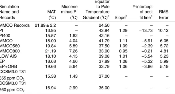
Table 1.Compilation of model and proxy MAT values, equator to pole temperature gradient values, and model data point wise comparison statistics.

Equator

Simulation Miocene to Pole Y-intercept

Name and MAT minus PI Temperature of best RMS

Records (◦_C) ₍◦_C) _{Gradient (}◦_C)a

Slopeb fit lineb Error

MMCO Records 21.89_±2.2 – 24.50 – – –

PI 13.95 – 43.84 1.29 ₋13.73 10.12

PI400 15.57 1.62 42.16 – – –

MMCO 18.00 4.04 41.79 1.11 ₋5.91 6.05

MMCO560 19.84 5.89 37.50 1.09 −2.39 5.72

MMCO800 21.19 7.26 33.00 0.95 −0.21 4.81

LOW AIS 18.10 4.15 39.08 1.01 −5.54 5.23

EP 18.68 4.66 37.89 1.08 −5.32 5.99

EP₊ORB 19.66 5.64 33.79 1.06 ₋3.86 5.19

CCSM3.0 T31

355 ppm CO₂ 15.38 1.43 37.00 – – –

CCSM3.0 T31

560 ppm CO₂ 16.94 2.99 35.00 – – –

a_{The equator to pole surface temperature gradient is calculated by averaging the mean annual temperatures over the}

absolute latitudes of (60–80◦_{) minus (0–30}◦_{); 80}◦_{is the maximum latitudinal extent of proxy records.}b_{The slope and}

(24)

CPD

9, 3489–3518, 2013

CESM1

A. Goldner et al.

Title Page

Tables Figures

◭ ◮

Back Close

Full Screen / Esc

Discussion

P

a

per

|

D

iscussion

P

a

per

|

Discussion

P

a

per

|

Discuss

ion

P

a

per

|

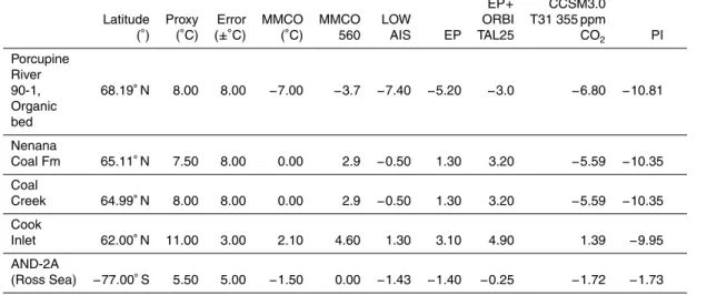
Table 2. High latitude model proxy data comparison for the Alaskan and Antarctic records. The simulations in the comparison include CESM1.0 and CCSM3.0 (Herold et al., 2011) model runs.

EP+ CCSM3.0 Latitude Proxy Error MMCO MMCO LOW ORBI T31 355 ppm

(◦₎ ₍◦_C) ₍

±◦C) (◦C) 560 AIS EP TAL25 CO2 PI

Porcupine River

90-1, 68.19◦_N _8.00 _8.00

−7.00 −3.7 −7.40 −5.20 −3.0 −6.80 −10.81 Organic

bed Nenana

Coal Fm 65.11◦_N _7.50 _8.00 _0.00 _2.9

−0.50 1.30 3.20 −5.59 −10.35 Coal

Creek 64.99◦_N _8.00 _8.00 _0.00 _2.9

−0.50 1.30 3.20 −5.59 −10.35

Cook

Inlet 62.00◦_N _11.00 _3.00 _2.10 _4.60 _1.30 _3.10 _4.90 _1.39

−9.95 AND-2A

(Ross Sea) ₋77.00◦_S _5.50 _5.00

(25)

CPD

9, 3489–3518, 2013

CESM1

A. Goldner et al.

Title Page

Tables Figures

◭ ◮

Back Close

Full Screen / Esc

Discussion

P

a

per

|

D

iscussion

P

a

per

|

Discussion

P

a

per

|

Discuss

ion

P

a

per

-10 0 10 20 30

-80 -40 0 40 80

Latitude

MAT

˚C

a

b

(26)

CPD

9, 3489–3518, 2013

CESM1

A. Goldner et al.

Title Page

Tables Figures

◭ ◮

Back Close

Full Screen / Esc

Discussion

P

a

per

|

D

iscussion

P

a

per

|

Discussion

P

a

per

|

Discuss

ion

P

a

per

|

High AIS

a

b

-10 0 10 20 30

Mo

d

e

lle

d

MAT

˚C

Proxy MAT ˚C Ocean

Terrestrial

Modelled ∆MAT from PI = 4.04˚C

(27)

CPD

9, 3489–3518, 2013

CESM1

A. Goldner et al.

Title Page

Tables Figures

◭ ◮

Back Close

Full Screen / Esc

Discussion

P

a

per

|

D

iscussion

P

a

per

|

Discussion

P

a

per

|

Discuss

ion

P

a

per

MMCO560 - MMCO _∆T = 1.84˚C

a

MMCO560

Modelled _∆MAT from PI = 5.89˚C

-10 0 10 20 30

Proxy MAT ˚C

Mo

d

e

lle

d

MAT

˚C

b

-10 0 10 20 30

Mo

d

e

lle

d

MAT

˚C

Proxy MAT ˚C MMCO800

d c

MMCO800 - MMCO _∆T = 3.19˚C

Fig. 3. (a)Modelled temperature anomaly for the MMCO560 (560 ppm CO₂) simulation minus the MMCO simulation (◦_C)._(b)_{Pointwise MMCO560 simulated global MAT compared against}

the proxy record MAT (◦_C). _(c) _{Modelled temperature anomaly for the MMCO800 (800 ppm}

CO₂) simulation minus the MMCO simulation (◦_C). _(d)_{Pointwise MMCO800 simulated global}

MAT compared against the proxy record MAT (◦_{C). These are the same terrestrial and SST}

(28)

CPD

9, 3489–3518, 2013

CESM1

A. Goldner et al.

Title Page

Tables Figures

◭ ◮

Back Close

Full Screen / Esc

Discussion

P

a

per

|

D

iscussion

P

a

per

|

Discussion

P

a

per

|

Discuss

ion

P

a

per

|

LOW AIS

a

LOW AIS-MMCO _∆T = 0.10˚C

b

LOW AIS

Modelled ∆MAT from PI = 4.15˚C

c

-10 0 10 20 30

Mo

d

e

lle

d

MAT

˚C

Proxy MAT ˚C

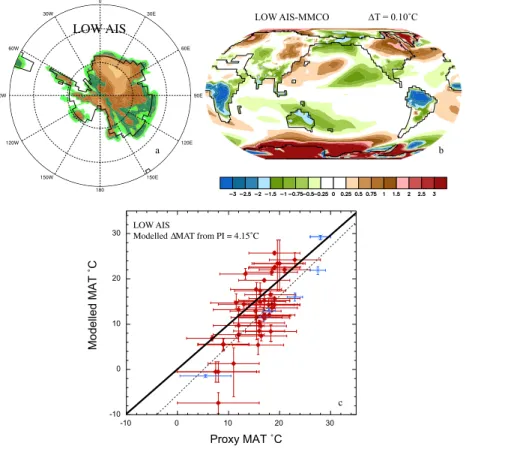
Fig. 4. (a)LOW AIS topography based on offline ice-sheet modeling (David Pollard, personal comms), (b) modelled temperature anomaly (◦_{C) between the LOW AIS simulation and the}

(29)

CPD

9, 3489–3518, 2013

CESM1

A. Goldner et al.

Title Page

Tables Figures

◭ ◮

Back Close

Full Screen / Esc

Discussion

P

a

per

|

D

iscussion

P

a

per

|

Discussion

P

a

per

|

Discuss

ion

P

a

per

∆T = 0.58˚C EP- LOW AIS

a

-10 0 10 20 30

Ocean Terrestrial

Mo

d

e

lle

d

MAT

˚C

Proxy MAT ˚C

b EP

Fig. 5. (a)Modelled temperature anomaly for the EP simulation minus the LOW AIS simulation (◦_C),_(b)_{Pointwise EP case global mean MAT compared against the proxy record MAT (}◦_C).

(30)

CPD

9, 3489–3518, 2013

CESM1

A. Goldner et al.

Title Page

Tables Figures

◭ ◮

Back Close

Full Screen / Esc

Discussion

P

a

per

|

D

iscussion

P

a

per

|

Discussion

P

a

per

|

Discuss

ion

P

a

per

|

EP + ORBITAL - LOW AIS _∆T = 1.53˚C

a

-10 0 10 20 30

Mo

d

e

lle

d

MAT

˚C

Proxy MAT ˚C Ocean

Terrestrial

EP + ORBITAL25

b

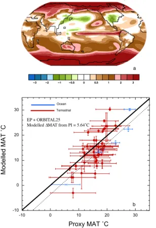
Fig. 6. (a)Modelled temperature anomaly for the EP₊ORBITAL25 simulation minus the LOW AIS simulation (◦_C),_(b)_{Pointwise EP}

+ORBITAL25 case global mean MAT compared against the proxy record MAT (◦_{C). These are the same terrestrial and SST records described in Fig. 1.}