Abstract— In this paper, an approximate formulation of the arbitrary order weakly singular integral is acquired by using Block-Pulse functions. The formulation contributes a numerical scheme for solving the higher order linear and nonlinear weakly singular Volterra integral equation of the second kind. By implementing the Block-Pulse functions and the approximation, the considered equations will be reduced to a system of algebraic equations. Also, the error analyses of the suggested numerical method are provided. Some examples are considered to demonstrate the efficiency and accuracy of proposed numerical approach.
Index Terms— weakly singular integral, weakly singular integral equation, Block Pulse functions, operational matrix, error analysis, numerical solution.
I. INTRODUCTION
NTEGRAL equations with higher order have recently proved to be valuable tools to the modeling of many physical phenomena and itstarts to attract much more attention of Physicists and Mathematicians [1-3]. These equations are represented by linear and nonlinear integral equations and solving such higher order integral equations is very important [4-10]. So it is very important to find efficient methods for solving higher order integral equations. The weakly singular Volterra integral equations are also found in a lot of physical, chemical, and biological problems, such as reaction-diffusion problems, crystal growth and so on [11-13]. Most of the higher order integral equations do not have exact analytical solutions; hence considerable need has been focused on approximate and numerical solutions of these equations.
Recently, various researchers have introduced new methods in the literature. These methods include operational matrix method [5], Adomian decomposition method (ADM) [7], differential transform method (DTM) [8], Laplace decomposition method (LDM) [10], homotopy analysis method (HAM) [14] and homotopy perturbation method (HPM) [15]. In this article, the integration operational matrix of the Block Pulse functions is got by using the operational matrix of Legendre wavelet. The operational matrix will be used to solve the higher order linear and nonlinear weakly singular Volterra integral equation.
In this paper, we describe application of Block Pulse
Manuscript received April 11, 2016; revised April 14, 2016.
Hao Song is with the School of Aeronautic Science and Technology, Beihang University, Beijing, P.R.China (e-mail: [email protected]).
Mingxu Yi is with the School of Aeronautic Science and Technology, Beihang University, Beijing, P.R.China (e-mail: [email protected]).
functions basis in solving the higher order linear and nonlinear Volterra integral equation with a weakly singular kernel. Consider the higher order linear Volterra integral equation with weakly singular kernel
( ) 0 0
( ) ( ) ( ) ( ) ( ).
n t
i i i
a t y t t s y s ds f t
(1) where a ti( ), ( )f t are known continuous functions on [0,1] and( )
( )
i
y t stands for the ith-order derivative of y t( ). is a real constants.
The higher order nonlinear Volterra integral equation with weakly singular kernel is as following
( ) 0 0
( ) ( ) ( ) [ ( )] ( ).
n t
i p
i i
a t y t t s y s ds f t
(2)II. THE QUADRATURE FORMULATION OF THE ARBITRARY ORDER WEAKLY SINGULAR INTEGRAL
Block Pulse functions have been studied by many authors and also have been applied for solving different problems. Here, we present a brief review of Block Pulse functions and its properties [15]. The m-set of Block Pulse functions are defined as
( 1)
1, ;
( )
0, .
i
iT i T
x
b x m m
otherwise
(3) where i0,1,2, m1,
with a positive integer value for m. In this paper, we setT1, and
( ), ;
( ) ( )
0 .
i
i j
b x i j
b x b x
i j
(4) The set of Block Pulse functions are orthogonal with each other, that is
1 0
1 / , ;
( ) ( )
0, .
i j
m i j
b x b x dx
i j
(5) As mtends to infinity, the m-set of Block Pulse functions become a complete basis for any 2[0,1)
L , so that an arbitrary real bounded function f t( ), which is square integrable in the interval [0, )T , can be expanded into
1 2 2 2
0
0f ( )x dx i fi b xi( ) .
(6)where 1
0 ( ) ( ) .
i i
f m b x f x dx
Arbitrary order weakly singular integral is given by as following
Numerical Solution of the Arbitrary Order
Weakly Singular Integral Equation Using Block
Pulse Functions
Hao Song and Mingxu Yi
I
Proceedings of the World Congress on Engineering 2016 Vol I WCE 2016, June 29 - July 1, 2016, London, U.K.
ISBN: 978-988-19253-0-5
ISSN: 2078-0958 (Print); ISSN: 2078-0966 (Online)
0
( )
( ) , 0 1, 0 1.
( )
t g s
I t ds t
t s
(7)where 2
( ) ([0,1])
g s L .
Using the orthogonality property of the Block-Pulse functions, the function g s( ) can be written as
1
0
( ) ( ) ( ).
m
T
i i m
i
g s c b s c B s
(8) where ( , ,0 1 , 1)T m
c c c c , ( ) ( ( ), ( ),0 1 , 1( )) T
m m
B x b s b s b s .
Substituting the Equation (8) into Equation (7), we have:
0 0
( ) ( )
( ) ( ).
( ) ( )
t T t T
m
g s B s
I t ds c ds c D t
t s t s
(9)where 0 ( ) ( ) . ( ) t m B s
D t ds
t s
(10) Combining Equation (3) and Equation (10), we can obtain0
1/ 2 /
0 1/ /
1 1 1 1
1 ( ) ( ) ( ) ( ) ( ) ( ) ( ) ( ) ( )
1 2 1
=( 1 1 0 0) 1 t m
m m t
m m m
m i m
T
B s
D t ds
t s
B s B s B s
ds ds ds
t s t s t s
t t t t
m m m
i t m
(11)where (0) (0,0, ,0)T
D .
Let tk m/ , k
1, 2, ,m1
, we have1 1
1 1 1
1 ( ) ( ) ( ) ( , 1 2 1 ( ) ( ) ( )
, , ,0, ,0) .
1 1
T
k k
k m m m
D m
k k k i
m m m m m m
At this time,i k 1.
Using Equation (9) and Equation (11), we can obtain the approximation of Equation (7).
III. METHOD OF SOLUTION
In this section, a collocation method based on Block Pulse functions is presented for solving the following linear weakly singular Volterra integral equation:
( ) 0 0 ( ) ( ) ( ) ( ) ( ). n t i i i
a t y t t s y s ds f t
(12) with condition( 1) ( 2)
1 2 0
(0) , (0) , , (0) ,
0 1, 0 1.
n n
n n
y y y y y y
t
(13)
where a ti( ), ( )f t are known continuous functions on [0,1]
and ( ) 2
( ) ([0,1])
i
y t L stands for the ith-order derivative of ( )
y t . andyk(k0,1,2, ,n1) are real constants.
Before solving Equation (12), the integration operational matrix of Block-Pulse functions can be got by using the operational matrix of Legendre wavelet.
Legendre wavelet in the interval [0,1)can be defined as [16-17]:
1 2 ( )
1
2 12 (2 2 1), [ , );
( ) 2 2
0, .
k k
k m k k
nm
n n
m P x n x
x
otherwise
(14)
m
P is said Legendre polynomial.
Set P is the Legendre wavelet operational matrix of integration,
where 1
2k
m m
L F F F
O L F F
P
O O O L F
O O O O L
,
2 0 0
0 0 0
0 0 0 M M
F and 1
1 0 0 0
3
1 3
0 0 0
3 3 5
3 5
0 0 0
3 5 5 7
7
0 0 0 0
5 5
2 3
0 0 0 0
(2 3) 2 5
0 0 0 0 0
0 0 0 0 0 0 0 0 , 2 3 0
(2 3) 2 1
2 1
0
(2 3) 2 5 M M
L M M M M M M M
M M
where 1
2k
m M. Let 1 2 1 2 i k i t M
, 1
1,2, ,2k
i M , the Legendre wavelet matrix [15] can be acquired
1
1 2 2
[ ( ), ( ), , ( k )].
m m t t t M
(15)
where
1 1
( ) ( ) ( )
1,0 1, 1 2,0
( ) ( ) ( )
2, 1 2 ,0 2 , 1
( ) [ ( ), , ( ), ( ), ,
( ), , k ( ), , k ( )] .
k k k
M
k k k T
M M
t t t t
t t t
The relation between the Block-Pulse functions and Legendre wavelet is given by
( )t m m B tm( ).
(16) Then we have
1 1
0 ( ) 0 ( ) ( ).
t t
m m m m m m m m
B s ds s ds P B t
(17)Let 1
m m m m
Q P , Q is called the Block-Pulse operational matrix of integration
0 ( ) ( ).
t
m m
B s dsQB t
(18) Suppose ( ) 2( ) ([0,1])
n
y t L , then we get
Proceedings of the World Congress on Engineering 2016 Vol I WCE 2016, June 29 - July 1, 2016, London, U.K.
ISBN: 978-988-19253-0-5
ISSN: 2078-0958 (Print); ISSN: 2078-0966 (Online)
1 ( )
0
( ) ( ) ( ).
m
n T
i i m
i
y t d b t d B t
(19)( 1) ( ) ( 1) ( 1)
0
( ) t ( ) (0) [ (0)] ( ).
n n n T T n
m
y t
y s dsy d QA y B t (20)( 2) 2 ( 1) ( 1)
( ) [ (0) (0)] ( ).
n T T n T n
m
y t d Q A y QA y B t (21)
……….
( 1) 1
( ) [ (0)
(0) (0)] ( ).
T n T n n
T T
m
y t d Q A y Q
A y Q A y B t
(22)
0,1, 2 ,
i n
,
( ) ( 1) 1 ( )
( ) [ (0) (0)] ( ).
i T n i T n n i T i
m
y t d Q A y Q A y B t (23)
where 1
0 m( )
Am B t dt
.Substituting the Equation (23), Equation (22) and Equation (9) into Equation (12), we can obtain.
0
( 1) 1 ( )
0
( 1) 1
( ( ) ( ) ( ))
( ) ( )( (0) (0)) ( )
( (0) (0)) ( ).
n
T n i n
i m
i n
T n n i T i
i m
i
T n n T
d a t Q B t Q D t
f t a t A y Q A y B t
A y Q A y D t
(24)Discreting the Equation (24) by taking step 1 m
oft, a linear system of algebraic equations can be easily got. Then
T
d can be got by solving Equation (24).
Consider the following nonlinear weakly singular Volterra integral equation:
( ) 0 0
( ) ( ) ( ) [ ( )] ( ).
n t
i p
i i
a t y t t s y s ds f t
(25)with the initial conditions Equation (13).
Let ( 1) 1
(0) (0) (0)
T T n T n n T T
d Q A y Q A y Q A y
, namely ( 0, 1, , 1)
T m
, Equation (22) can be rewritten as
( ) T ( ).
m
f t B t (26) Using the properties of the Block-Pulse functions, Equation (27) can be got.
[ ( )]p [ p T] ( ).
m
f t B t (27) where ( 0, 1, , 1)
p p p p T
m
.
Substituting the Equation (23), Equation (27) and Equation (9) into Equation (25), we have:
0
( 1) 1
0
( ) ( ) [ ] ( )
( ) ( )( (0) ) ( ).
n
T i p T
i m
i
n
T i T i
i m
i
a t Q B t D t
f t a t A y Q A y Q B t
(28)when p1, Equation (28) is Equation (24). Discreting the Equation (28) by taking step 1
m
of t, a nonlinear system of algebraic equations can be easily got. Then andy t( )can be also obtained.
IV. ERROR ANALYSIS
In this section, we analyze the error when a differentiable function y x( ) is represented in a series of block pulse functions over the intervalI[0,1). We need the following theorem.
Theorem 4.1 Suppose y x( ) is continuous in I , is
differentiable in (0,1) , and there is a number M such that y x( ) M, for everyxI. Then
( ) ( )
y b y a M ba , for all a b, I.
Now, we assume that y x( )is a differentiable function on I such that y x( ) M. We define the error between y x( )and its block pulse functions expansion over every subinterval Iias
follows:
( ) ( ), .
i i i
e x c y x xI (29)
where i , 1
i i I
n n
. It can be shown that
( 1) /
2 2 2
/
1
( ) ( ( )) , .
i n
i i n i i i
e e x dx c y I
n
(30) where we used mean value theorem for integral. Using Equation (6) and the mean value theorem, we have( 1) / /
1
( ) ( ) ( ), .
i n
i i n i
c n y x dx n y y I
n
(31) Substituting Equation (31) into Equation (30) and using Theorem 4.1, we have2 2
2 2 2
3
1
( ( ) ( )) .
i
M M
e y y
n n n
(32) This leads to
2 1
1 1
2 2
0 0
0 1
1 1
2
0 0
0
( ) ( ) ( )
( ) 2 ( ) ( ) .
n i i n
i i j
i i j
e x e x dx e x dx
e x dx e x e x dx
(33)
Since fori j I, i Ij , then
1 1 1
2 2 2
0
0 0
( ) ( ) .
n n
i i
i i
e x e x dx e
(34) Substituting Equation (33) into Equation (34), we get2 2
2
( ) M .
e x n
(35)
hence, e x( ) O 1 n
, where e x( )y xn( )y x( )and
1
0
( ) ( )
n
n i i
i
y x c b x
.V. NUMERICAL EXAMPLES
Example 1. Consider the weakly singular integral [18]
1( ) 0 .
n
t s
I t ds
t s
(36)The exact solution is
1
( )
2 ( 1)
3
( )
2
n
t n
n
. Taking
64, 128,
m m and making use of MATLAB2011a, Fig. 1
and Fig. 2 are comparison of the numerical solutions with the
exact.
Proceedings of the World Congress on Engineering 2016 Vol I WCE 2016, June 29 - July 1, 2016, London, U.K.
ISBN: 978-988-19253-0-5
ISSN: 2078-0958 (Print); ISSN: 2078-0966 (Online)
Fig. 1. m64,n =4.
Fig. 2. m128,n =4.
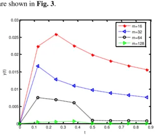
Example 2. Consider the weakly singular Volterra integral
equation [20]:
1/ 2 0
1
( ) ( )( ) , 0 1.
2
t
y t
y s ts ds t t t (37) The exact solution is t. The absolute errors for differentmare shown in Fig. 3.
0 0.1 0.2 0.3 0.4 0.5 0.6 0.7 0.8 0.9 0
0.005 0.01 0.015 0.02 0.025 0.03
t
y
(t
)
m=16 m=32 m=64 m=128
Fig. 3. The absolute errors for differentm.
VI. CONCLUSION
In this work, the Block-Pulse functions and their good properties has been successfully applied to construct approximate solutions for higher order linear and nonlinear weakly singular Volterra integral equation of the second kind. The Block-Pulse functions method provides the solution in terms of convergent series with easily computable
components. The approximation of the arbitrary order weakly singular integral and integration operational matrix are obtained. The initial equations can be transformed into a system of algebraic equations. The Block-Pulse functions method is effective and simple to solve the higher order linear and nonlinear weakly singular Volterra integral equation.
ACKNOWLEDGMENT
The authors are very thankful to the reviewers and the editors of this paper for their constructive comments and nice suggestions, which helped to improve the paper.
REFERENCES
[1] Domenico Mucci, “A characterization of graphs which can be approximated in area by smooth graphs”, Journal of the European Mathematical Society, 3(1) (2001):1-38.
[2] Yu Xiulan, Zhu Chun, Wang, JinRong, “On a weakly singular quadratic integral equations of Volterra type in Banach algebras”, Advances in Difference Equations, 1(2014):1-18. [3] D.Yu(2002), Natural Boundary Integral Method and its Application,
Science Press, Kluwer Academic Publishers, Beijing(2003). [4] P.K. Kythe, Computational Methods for Linear Integral Equations,
Bikhauser, Boston(2002).
[5] B.Q. Tang, X.F. Li, “Solution of a class of Volterra integral equations with singular and weakly singular kernel”, Applied Mathematics and Computation, 199(2008):406-413.
[6] Zhong Chen, YingZhen Lin, “The exact solution of a linear integral equation with weakly singular kernel”, J.Math. Anal. Appl., 344(2008):726-734.
[7] B.N. Mandal, G. Bera, “Approximate solution of a class of singular integral equations of second kind”, J. Comput. Appl. Math., 206(2007):189-195.
[8] M.A. Abdou, A.A.Nasr, “On the numerical treatment of the singular integral equation of the second kind”, Applied Mathematics and Computation, 146(2003):373-380.
[9] Tomoaki Okayama, “Sinc-collocation methods for weakly singular Fredholm integral equations of the second kind”, J. Comput. App. Math., 234(2010):1211-1227.
[10] Arvet Pedas, “A discrete collocation method for Fredholm integro-differential equations with weakly singular kernels”, Applied Numerical Math., 61(2011):738-751.
[11] R. Gorenflo, Abel Integral Equations-Analysis and Applications, Spinger, Berlin (1991).
[12] E.G. Ladopoulos, Singular Integral Equations linear and nonlinear Theory and its Application in Science and Engineering, Springer-Verlag, Berlin, Heidelberg, Germany(2000).
[13] M.Rasty, “A product integration approach based on new orthogonal polynomials for nonlinear weakly singular integral equations”, Acta Appl. Math., 109(2010):861-873.
[14] E.Babolian, Z.M, “Numerical solution of nonlinear Volterra-Fredholm Integro-differential equations via direct method using triangular functions”, Comp. Math with Appl., 58(2009):239-247.
[15] H. Saeedi, “A CAS wavelet method for solving nonlinear Fredholm integro-differential equation of fractional order”, Communications in Nonlinear Science and Numerical Simulation, 16(2011):1154-1163. [16] Y.J. Shen, W. Lin, “Collocation method for the natural boundary
integral equation”, Appl. Math. Letters, 19(2006):1278-1285. [17] S. Zhi, Z.Q. Deng, “Legendre wavelet for Fredholm
Intergro-differential equation”, J. Math. Study, 42(4) (2009):411-417. [18] Sohrab Ali, “Numerical solution of Abel’s integral equation by using Legendre wavelets”, Applied Mathematics and Computation, 175(2006):574-580.
[19] Osman Rasit Isik, M. Sezer, “Bernstein series solution of a class of linear integro-differential equations with weakly singular keener”, Applied Mathematics and Computation, 217(2011):7009-7020. [20] Paola Baratella, “A new approach to the numerical solution of weakly
singular Volterra integral equations”, J. Comput. Appl. Math., 163(2004):401-418.
Proceedings of the World Congress on Engineering 2016 Vol I WCE 2016, June 29 - July 1, 2016, London, U.K.
ISBN: 978-988-19253-0-5
ISSN: 2078-0958 (Print); ISSN: 2078-0966 (Online)