www.biogeosciences.net/13/4789/2016/ doi:10.5194/bg-13-4789-2016
© Author(s) 2016. CC Attribution 3.0 License.
Greenhouse gas emissions from natural ecosystems and agricultural
lands in sub-Saharan Africa: synthesis of available data and
suggestions for further research
Dong-Gill Kim1, Andrew D. Thomas2, David Pelster3, Todd S. Rosenstock4, and Alberto Sanz-Cobena5 1Wondo Genet College of Forestry and Natural Resources, Hawassa University, P.O. Box 128, Shashemene, Ethiopia 2Department of Geography and Earth Sciences, Aberystwyth University, Aberystwyth SY23 3DB, UK
3International Livestock Research Institute, P.O. Box 30709, Nairobi, Kenya
4World Agroforestry Centre (ICRAF), P.O. Box 30677-00100, United Nations Avenue, Nairobi, Kenya 5Technical University of Madrid, School of Agriculture, Avd. Complutense s/n, 28040 Madrid, Spain
Correspondence to:Dong-Gill Kim (donggillkim@gmail.com)
Received: 6 September 2015 – Published in Biogeosciences Discuss.: 9 October 2015 Revised: 23 July 2016 – Accepted: 3 August 2016 – Published: 29 August 2016
Abstract. This paper summarizes currently available data on greenhouse gas (GHG) emissions from African natural ecosystems and agricultural lands. The avail-able data are used to synthesize current understanding of the drivers of change in GHG emissions, outline the knowledge gaps, and suggest future directions and strate-gies for GHG emission research. GHG emission data were collected from 75 studies conducted in 22 coun-tries (n=244) in sub-Saharan Africa (SSA). Carbon dioxide (CO2) emissions were by far the largest con-tributor to GHG emissions and global warming potential (GWP) in SSA natural terrestrial systems. CO2 emis-sions ranged from 3.3 to 57.0 Mg CO2ha−1yr−1, methane (CH4) emissions ranged from −4.8 to 3.5 kg ha−1yr−1 (−0.16 to 0.12 Mg CO2 equivalent (eq.) ha−1yr−1), and nitrous oxide (N2O) emissions ranged from −0.1 to 13.7 kg ha−1yr−1 (−0.03 to 4.1 Mg CO
2 eq. ha−1yr−1). Soil physical and chemical properties, rewetting, veg-etation type, forest management, and land-use changes were all found to be important factors affecting soil GHG emissions from natural terrestrial systems. In aquatic systems, CO2 was the largest contributor to total GHG emissions, ranging from 5.7 to 232.0 Mg CO2ha−1yr−1, followed by −26.3 to 2741.9 kg CH4ha−1yr−1 (−0.89 to 93.2 Mg CO2eq. ha−1yr−1)and 0.2 to 3.5 kg N2O ha−1yr−1 (0.06 to 1.0 Mg CO2eq. ha−1yr−1). Rates of all GHG emis-sions from aquatic systems were affected by type, location,
from SSA natural ecosystems and agricultural lands were 56.9±12.7×10⁹Mg CO2eq. yr−1with natural ecosystems and agricultural lands contributing 76.3 and 23.7 %, respec-tively. Additional GHG emission measurements are urgently required to reduce uncertainty on annual GHG emissions from the different land uses and identify major control fac-tors and mitigation options for low-emission development. A common strategy for addressing this data gap may include identifying priorities for data acquisition, utilizing appropri-ate technologies, and involving international networks and collaboration.
1 Introduction
Global greenhouse gas (GHG) emissions were estimated to be 49×109Mg CO2 eq. in 2010 (IPCC, 2014), with approximately 21.2–24 % (10.3–12×109Mg CO2 eq.) of emissions originating from soils in agricultural, forestry and other land use (AFOLU; Tubiello et al., 2015; IPCC, 2014). Annual non-CO2 GHG emissions (primar-ily CH4 and N2O) from agriculture were estimated to be 5.2–5.8×10⁹Mg CO
2 eq. yr−1 in 2010 (FAOSTAT, 2015; Tubiello et al., 2013), with approximately 4.3– 5.5×10⁹Mg CO2 eq. yr−1 attributable to land-use change (IPCC, 2014).
Greenhouse gas fluxes in Africa play an important role in the global GHG budget (Thompson et al., 2014; Hick-man et al., 2014; Valentini et al., 2014; Ciais et al., 2011; Bombelli et al., 2009). For example, CO2eq. emissions from 12 river channels in SSA and wetlands of the Congo River were 3.3×10⁹Mg CO2eq. per year, equivalent to ca. 25 % of the global terrestrial and ocean carbon sink (Borges et al., 2015). Nitrous oxide emissions in SSA contribute between 6 and 19 % of the global total, and changes in soil N2O fluxes in SSA drive large interannual variations in tropical and sub-tropical N2O sources (Thompson et al., 2014; Hickman et al., 2011). Use of synthetic fertilizers such as urea has in-creased in the last four decades, as has the number of live-stock (and their manure and urine products) in Africa (Bouw-man et al., 2009, 2013). The increasing trend in N applica-tion rates is expected to cause a 2-fold increase in agricul-tural N2O emissions in the continent by 2050 (from 2000; Hickman et al., 2011). In the case of CH4emissions, there are important differences between ecosystems. Tropical hu-mid forest, wetlands, rice paddy fields, and termite mounds are likely sources of CH4, while seasonally dry forests and savannahs are typically CH4sinks (Valentini et al., 2014).
Interpretation of GHG emissions from soils and terrestrial water bodies is complex because of the multiple, sometimes competing, biological, chemical, and physical processes af-fecting fluxes. Spatial and temporal variability in GHG fluxes is also high and challenging to capture with direct measure-ment. This in turn makes reliable annual GHG flux estimates
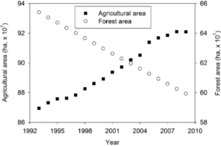
Figure 1. Change in areas of agricultural land and forest
in Africa. Data source: FAOSTAT, http://faostat.fao.org/site/377/ default.aspx#ancor.
Our current understanding of GHG emissions in SSA is particularly limited when compared to the potential the con-tinent has as both a GHG sink and a source. This lack of data on GHG emissions from African natural and agricul-tural lands and the lack of a comprehensive analysis of ex-isting data (i.e., type of emission drivers: natural factors or anthropic ones) hinder the progress of our understanding of GHG emissions on the continent (Hickman et al., 2014; Valentini et al., 2014; Ciais et al., 2011; Bombelli et al., 2009). In order to identify mitigation measures and other climate-smart interventions for the region, it is important to quantify baseline GHG emissions, as well as understand the impacts of different land-use management strategies on GHG emissions (e.g., Palm et al., 2010). In this study our objec-tives are to synthesize currently available data on GHG emis-sions in natural ecosystems and agricultural lands in SSA, create an inventory of information from studies on emissions, and select priority topics for future GHG emission studies in natural ecosystems and agricultural lands in SSA.
2 Methodology
2.1 Data collection and analyses
Data were acquired by searching existing peer-reviewed lit-erature using the names of the sub-Saharan countries and the GHGs (i.e., CO2, CH4, N2O) as search terms (using Web of Science and Google Scholar; 1960–2015). These criteria yielded 310 peer-reviewed papers. To produce the quantitative summary of GHG emissions, we selected stud-ies that reported in situ annual GHG emissions or those that provided enough information to estimate annual GHG emissions through unit conversion and/or extrapolation of given data. Data from 75 studies, conducted in 22 coun-tries (n=244) in SSA, were used and were further cate-gorized as GHG emission in natural ecosystems (n=117; Supplement Table S1) and agricultural lands (n=127; Ta-ble S2; Fig. 2). The category of GHG emissions in natural ecosystems were further divided into emissions from natural terrestrial systems (forest/plantation/woodland (n=55), sa-vannah/grassland (n=31), termite mounds (n=5), and salt pans (n=1)) and aquatic systems (streams/rivers (n=14), wetlands/floodplains/lagoons/reservoirs/lakes (n=11)) (Ta-ble 1). Greenhouse gas emissions in agricultural lands were subdivided into emissions from cropland (n=105), rice pad-dies (n=1), vegetable gardens (n=5), and agroforestry (n=16; Table 1). Across all categories there were 174 CO2, 201 CH4, and 184 N2O emissions measurements. To allow comparison between different GHG emissions CH4 and N2O emissions were converted to CO2 eq. assuming a 100-year global warming potential and values of 34 and 298 kg CO2eq. for CH4and N2O, respectively (IPCC, 2013). Where N2O emission studies included experimental data from control plots with no N fertilizer additions (i.e., for
background N2O emissions), and from plots with different levels of applied N, a N2O emission factor (EF) was calcu-lated following the IPCC (2006) Tier I methodology as fol-lows:
N2O EF(%)=
N2O emissionN treatment−N2O emissioncontrol Ninput
×100, (1)
where N2O EF (%) is N2O emission factor, N2O emissionN treatment is N2O emission in N input, N2O emissioncontrolis control treatments with no N fertilizer ad-ditions, and Ninputis the amount of added N.
It should be noted that our data compilation includes a wide variety of studies that were conducted under diverse biophysical conditions using a range of methodologies for quantifying GHG emissions (e.g., different sampling proto-cols, chamber design, and emission rate calculations), soil properties, and climatic factors. Therefore, the overall figures on GHG emissions shown are based on results achieved by different measurement techniques with inherent and contrast-ing sources of error. To assess data quality of the cited stud-ies we used the criteria (ranked from “very poor” to “very good”) suggested by Rochette and Eriksen-Hamel (2008). These were originally intended for chamber N2O measure-ments but are equally applicable to field-based CO2and CH4 chamber measurements. We went through the methods of the papers used in the study (only those for terrestrial emissions, since these criteria are not applicable for aquatic systems) where there was sufficient detail in the methods section. We categorized the studies as three different groups: the methods are (1) poor to very poor, (2) marginal and (3) good. Studies that were ranked “poor” on 3 or more criteria or “very poor” on 2 or more criteria were categorized as such because the methods were poor to very poor. In addition, we took into account the importance of sampling frequency (Barton et al., 2015) and sampling periods. Studies estimating annual GHG emissions with a sampling frequency lower than biweekly (i.e., less than two times per month) and sampling periods of less than 6 months (i.e., covering both rainy and dry sea-sons) were also categorized as poor to very poor. Studies that were ranked as “poor” on two criteria, or “very poor” on one criterion, or with insufficient details on the methods were ranked as marginal. The good studies were those with only one “poor” ranking, sufficient detail, and a sampling fre-quency of every 2 weeks or more frequent.
2.2 Statistical analyses
Table 1.Summary of greenhouse gas carbon dioxide (CO2), methane (CH4), nitrous oxide (N2O), emissions and CO2equivalents (CO2eq.)
in natural ecosystems and agricultural lands in sub-Saharan African countries. Mean±standard error (number of data) are shown.
CO2emission CH4emission N2O emission N2O emission CO2eq. Total CO2eq. factor emission emission
Type Area (Mha) Mg CO2ha−1yr−1 kg CH4ha−1yr−1 kg N2O ha−1yr−1 % Mg CO2eq
.ha−1yr−1 ×10iMg CO2eq.yr−1 Forest/plantation/woodland 740.6a 32.0±5.0 (34) −1.5±0.6 (15) 4.2±1.5 (10) d 34.0±5.7 25.2±4.2 Savannah/grassland 638.9a 15.5±3.8 (11) 0.5±0.4 (18) 0.6±0.1 (6) d 15.8±3.8 10.1±2.4 Stream/river 28.2a 78.1±13.2 (27) 436.3±133.8 (24) 1.6±0.3 (17) d 93.4±17.9 2.8±1.0 Wetlands/floodplains/lagoons/reservoir 43.8a 96.6±31.0 (7) 950.4±350.4 (5) 2.0±1.5 (2) d 121.3±39.7 5.3±1.7 Termite mounds 0.97b 11.6±6.2 (3) 2.3±1.1 (3) 0.01 (1) d 11.7±6.3 0.01±0.01
Salt pan d 0.7 (1) d d d d d
Total natural ecosystemsh 1452.5 27.6±2.9e 43.0±5.8e 2.5±0.4e d 29.9±22.5e 43.4±9.3 (76.3 %)g Cropland 468.7a 23.4±5.1 (45) 19.3±4.2 (26) 4.0±1.5 (83) 0.5±0.2 (24) 26.1±6.0 12.2±2.8 Rice field 10.5c 6.5 (1) 30.5 (1) 0.19 (1) d 7.3 1.3±0.6 Vegetable gardens d 96.4±10.2 (5) d 120.1±26.1 (5) 3.5±0.5 (2) d d Agroforestry 190f 38.6 (1) d 4.7±2.2 (15) d d d Total agricultural landsi 479.2 23.0±8.5e 19.5±5.6e 4.5±2.2e d 25.6±12.4e 13.5±3.4 (23.7 %)g Total natural ecosystems 1931.7 56.9±12.7 and agricultural landsj
aGlobCover 2009.b0.07 % of savannah and rainforest (Brümmer et al., 2009).cFAO STAT (http://faostat3.fao.org/home/E), year 2012.dNo data available.eArea-weighted average.fZomer et al. (2009).gContribution to CO
2eq. emission in total natural and agricultural lands.hExcept salt pan.iExcept vegetable gardens and agroforestry.jExcept salt pan, vegetable gardens, and agroforestry.
Savannah / grassland Streams / rivers Wetland / floodplain / lagoons Termite mounds Salt pans
Forest / plantation / woodland Croplands
Rice paddies Vegetable garden Agroforestry
Figure 2.Maps showing study sites of CO2, CH4, and N2O fluxes in natural ecosystems (left) and agricultural lands (right) in sub-Saharan
Africa.
natural log, logarithm, and sigmoidal) were tested for each dataset. The regression models were checked for violation of assumptions of normal distribution (Shapiro–Wilk test), homoscedasticity (Breusch–Pagan test), and constant vari-ance (Durbin–Watson statistic; Motulsky and Christopoulos, 2004). Separate t tests were used to assess significance of regression coefficients and intercepts in the fitted parametric models. Adjusted coefficients of determination (adjustedR2)
of fitted parametric models were used as criteria for model selection: the model with the highest adjusted R2 was se-lected. Statistical significance was considered at the critical level of 5 %. Statistical analyses were conducted using SAS®
version 9.2 (SAS Institute, Cary, NC, USA) and SigmaPlot® version 11.0 (Systat Software Inc., San Jose, CA, USA).
3 Results and discussion
3.1 Summary of greenhouse gas emissions 3.1.1 CO2emissions
in aquatic systems. The area-weighted average was 27.6±17.2 Mg CO2ha−1yr−1 (Tables 1 and S1). Aquatic systems such as water bodies or water submerged lands were the largest source of CO2, followed by forest, savannah, termite mounds, and salt pans (Table 1). Soil CO2emissions in agricultural lands were similar to emissions from natural lands and ranged from 6.5 to 141.2 Mg CO2ha−1yr−1with an area-weighted average of 23.0±8.5 Mg CO2ha−1yr−1 (Tables 1 and S2). Vegetable gardens were the largest sources of CO2 emission largely due to the excessive C inputs. However, this conclusion was based on two studies that used photoacoustic spectroscopy, which has been found have mixed results due to cross sensitivities between the various GHG and water vapor (Rosenstock et al., 2013; Iqbal et al., 2013), suggesting that vegetable gardens require further study. The next largest sources of emissions were agroforestry, cropland, and then rice production systems (Tables 1 and S2).
Observed annual soil CO2 emissions in African natural terrestrial systems and agricultural lands showed significant correlations with annual mean air temperature (r= −0.322,
P =0.01), annual rainfall (r=0.518, P< 0.001), SOC (r=0.626,P< 0.001), and soil total N content (r= 0.849,
P < 0.001; Table 2). The negative relationship between an-nual soil CO2 emissions and annual mean air tempera-ture was unexpected since positive correlations between soil CO2 flux and temperature are well established (e.g., Bond-Lamberty and Thomson, 2010). We speculate that the gen-erally high temperatures, and poor quality, of many African soils mean that air temperature increases frequently result in vegetation stress and/or soil aridity, hindering root and soil microbial activities (root and microbial respiration) and sub-sequent soil CO2flux (e.g., Thomas et al., 2011). This would account for the negative relationship observed between an-nual mean air temperature and anan-nual soil CO2 emissions, but this remains a largely untested hypothesis that deserves further exploration.
Many of these estimates are based on short-term, infre-quent, or poor-quality sampling (Table S1), suggesting that the uncertainties are likely much greater than the provided standard error. This is not meant as a critique of these stud-ies, as many of them were specifically designed to answer specific research questions about the effects of various fac-tors on emission rates rather than determining the cumula-tive annual emissions. However, given the lack of other data, these still provide the “best guess” for cumulative emissions.
3.1.2 CH4emissions
Forest/plantation/woodland were sinks of CH4 (−1.5±0.6 kg CH4ha−1yr−1) and savannah/grassland, croplands, termite mounds, and rice fields were low to moderate CH4 sources (0.5–30.5 kg CH4ha−1yr−1). Stream/river and wetland/floodplain/lagoon/reservoir were high CH4sources (766.0–950.4 kg CH4ha−1yr−1; Tables 1
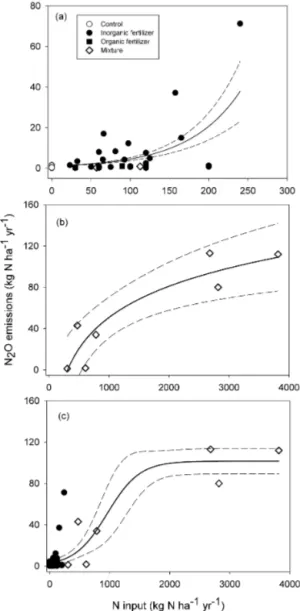
Figure 3.Relationship between nitrogen (N) input and nitrous
ox-ide (N2O) emissions observed in Africa. N input ranged from 0 to
300(a), 300 to 4000(b), and 0 to 4000 kg N ha−1yr−1 (c). The dashed lines indicate 95 % confidence intervals. “Control” indicates no fertilizer application, Organic fertilizer is manure; “Inorganic fertilizer” includes NPK, ammonium nitrate, and urea fertilizers; and “Mixture” indicates mixed application of organic and inorganic fertilizers.
and S1). The area-weighted averages of CH4 emissions from natural and agricultural lands were 43.0±5.8 and 19.5±5.6 kg CH4ha−1yr−1, respectively. As with studies on CO2 emissions, many of these studies used only infre-quent or poor sampling methodologies (Table S1), and there is a high degree of uncertainty surrounding the estimates.
3.1.3 N2O emissions and emission factor (EF)
Nitrous oxide emissions in natural ecosystems ranged from
aver-Table 2.Correlation between annual soil CO2emissions (Mg CO2ha−1yr−1)and environmental factors in African natural terrestrial
sys-tems.
Annual mean air Annual Soil organic Soil total
temperature (◦C) rainfall (mm) carbon (%) nitrogen (%)
Correlation coefficient −0.322 0.518 0.626 0.849
P value 0.01 < 0.001 < 0.001 < 0.001
Number of samples 60 61 31 26
age was 2.5±0.8 kg N2O ha−1yr−1 (Tables 1 and S1). Our study reveals that forest, plantation, and woodland were the largest source of N2O, followed by rivers and wetlands, savannah, and termite mounds in natural ecosystems (Ta-ble 1). Soil N2O emissions in agricultural lands ranged from 0.051 to 177.6 kg N2O ha−1yr−1and the area-weighted aver-age was 4.5±2.2 kg N2O ha−1yr−1 (Tables 1 and S2). The largest N2O source in agricultural lands was vegetable gar-dens, followed by agroforestry, cropland, and rice fields (Ta-ble 1). The N2O EF was 0.5±0.2 and 3.5±0.5 % for crop-land and vegetable gardens, respectively (Tables 1 and S1). The N2O EF of cropland is lower and the N2O EF of veg-etable gardens is higher than IPCC default N2O EF (1 %; IPCC, 2006). The number of studies on N2O emissions in SSA is, however, particularly low (n=14), with some ques-tions regarding the quality of the methods (Table S1) in some of these studies, and there are significant regional gaps lead-ing to large uncertainties in the conclusions that can be cur-rently drawn.
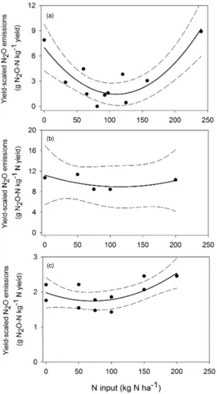
N2O emissions were significantly affected by N in-put levels (Fig. 3). N2O emissions increase slowly up to 150 kg N ha−1yr−1, after which emissions increase exponen-tially up to 300 kg N ha−1yr−1 (Fig. 3a). Consistent with earlier work by Van Groenigen et al. (2010), N inputs of over 300 kg N ha−1yr−1resulted in an exponential increase in emission (Fig. 3b), slowing to a steady state with N in-puts of 3000 kg N ha−1yr−1. Overall, the relationship be-tween N input and N2O emissions shows a sigmoidal pat-tern (Fig. 3c). The observed relationship is consistent with the proposed hypothetical conceptualization of N2O emis-sion by Kim et al. (2013), showing a sigmoidal response of N2O emissions to N input increases. The results suggest that N inputs over 150 kg N ha−1yr−1may cause an abnormal in-crease in N2O emissions in SSA. The relationship between N input and N2O emissions shows that the lowest yield-scaled N2O emissions were reported for N application rates ranging from 100 to 150 kg N ha−1 (Fig. 4). The results are in line with the global meta-analysis of Philiber et al. (2012), who showed that from an N application rate∼150 kg N ha−1the increase in N2O emissions is not linear but exponential.
3.1.4 CO2eq. emission
Carbon dioxide equivalent emission (including CO2, CH4, and N2O) in natural ecosystems ranged from 11.7 to
121.3 Mg CO2 eq. ha−1yr−1 and the area-weighted av-erage of CO2 eq. emissions (excluding salt pans) was 29.9±22.5 Mg CO2 eq. ha−1yr−1 (Table 1). Water bod-ies or water submerged lands such as rivers and wet-lands were the largest source of CO2 eq. emissions, fol-lowed by forest/plantation/woodland, savannah/grassland, and termite mounds (Table 1). Carbon dioxide equiv-alent emissions in agricultural lands ranged from 7.3 to 26.1 Mg CO2 eq. ha−1yr−1 and had an area-weighted average of CO2 eq. emissions (excluding vegetable gardens and agroforestry due to lack of data) of 25.6±12.4 Mg CO2eq. ha−1yr−1(Table 1).
Total CO2 eq. emissions in natural lands (exclud-ing salt pans) were 43.4±9.3×10⁹Mg CO2 eq. yr−1, with forest/plantation/woodland the largest source, followed by savannah/grassland, stream/river, wet-lands/floodplains/lagoons/reservoir, and termite mounds (Table 1). Total CO2 eq. emissions in agricultural lands (excluding vegetable gardens and agroforestry) were 13.5±3.4×10⁹Mg CO2eq. yr−1, with cropland the largest source, followed by rice fields (Table 1). Overall, total CO2 eq. emissions in natural ecosystems and agricultural lands were 56.9±12.7×10⁹Mg CO
2eq. yr−1with natural ecosystems and agricultural lands contributing 76.3 and 23.7 %, respectively.
3.1.5 Data quality assessment
(a)
(b)
(c)
-Figure 4.Relationship between nitrogen (N) input and yield scaled
nitrous oxide (N2O) emissions. Grain type:(a)rape (Brassica
na-pus) and(b, c) maize (Zea maysL.). Data sources:(a)from
Nya-madzawo et al. (2014a),(b)from Hickman et al. (2014) and(c)from
Hickman et al. (2015). The dashed lines indicate 95 % confidence intervals. Note the different scales across panels.
3.2 Sources and drivers of greenhouse gas emissions in Africa
3.2.1 Greenhouse gas emissions in natural ecosystems Natural terrestrial systems
A range of factors affect direct emissions of soil CO2 in SSA natural terrestrial systems such as natural forest, plan-tation, woodland, savannah, grassland, termite mounds, and salt pans. These factors can be grouped into (i) climatic, (ii) edaphic, (iii) vegetation, and (iv) human interventions via land management (Tables 3 and 4). Data on the effects of these factors on GHG emissions are variable, with some factors much less well understood than others. In almost all cases data are limited to a few studies, and there are areas where there has been no research. This lack of data hinders
our ability to estimate the contribution of African landscapes to global GHG emissions.
Soil CO2emissions were related to both soil moisture and temperature in forest systems (Table 3). For example, soil moisture explained about 50 % of the seasonal variability in soil CO2 efflux in aCroton macrostachys,Podocarpus
fal-catus, and Prunus africanaforest in Ethiopia (Yohannes et al., 2011), as well as much of the seasonal variation in soil CO2 efflux in a 3-year-oldEucalyptusplantation in the Re-public of Congo (Epron et al., 2004). Thomas et al. (2011) found that the Q10of soil CO2efflux (a measure of the tem-perature sensitivity of efflux, where a Q10 of 2 represents a doubling of efflux given a 10◦C increase in temperature) was dependent on soil moisture at sites across the Kalahari in Botswana, ranging from 1.1 in dry soils to 1.5 after a 2 mm rainfall event and 1.95 after a 50 mm event. Similarly, in a Zambian woodland, the main driving factor controlling CO2 emissions at a seasonal timescale was a combination of soil water content and temperature (Merbold et al., 2011).
Increased GHG emissions following rewetting of dry soil were observed in various regions in SSA (Table 3). Two broad mechanisms responsible for increased soil GHG flux following rewetting of dry soil have been hypothesized: (1) enhanced microbial metabolism by an increase in avail-able substrate due to microbial death and/or destruction of soil aggregates (commonly known as the Birch effect; Birch, 1964), and (2) physical mechanisms influencing gas flux, including infiltration, reduced diffusivity, and gas displace-ment in the soil (e.g., Kim et al., 2012). Soil CO2 efflux increased immediately after rainfall in a subtropical palm woodland in northern Botswana; however, the increase was short-lived (Thomas et al., 2014). Large pulses of CO2 and N2O, followed by a steady decline, were also observed after the first rainfall event of the wet season in a Kenyan rain-forest (Werner et al., 2007). Soil CO2 efflux was strongly stimulated by addition of rainfall in a South African savan-nah (Fan et al., 2015; Zepp et al., 1996). In Zimbabwe, the release of N2O from dryland savannahs was shown to con-stitute an important pathway of release for N, and emissions were strongly linked to patterns of rainfall (Rees et al., 2006). The results suggest that soil rewetting has a significant im-pact on GHG emissions in SSA.
high-Table 3.Summary of environmental factors affecting greenhouse gas (GHG) emissions in land-use/ecosystem type.◦indicates GHG affected by environmental factor named.
GHG
Land-use/ecosystem type Environmental factors CO2 N2O CH4 Location (data source)
Forest/plantation/ Temperature • Zambia (Merbold et al., 2011)
Woodland Soil moisture • Ethiopia (Yohannes et al., 2011),
Republic of Congo (Epron et al., 2004), Botswana (Thomas et al., 2011), Zambia (Merbold et al., 2011)
Rewetting of dry soil/rainfall • • Kenya (Werner et al., 2007)
Soil carbon • Zambia (Merbold et al., 2011),
Kenya (Werner et al., 2007)
Soil nitrogen • Kenya (Werner et al., 2007)
Soil C : N • Kenya (Werner et al., 2007)
Soil clay • Kenya (Werner et al., 2007)
Soil bulk density • Rwanda (Gharahi Ghehi et al., 2014)
Soil pH • Rwanda (Gharahi Ghehi et al., 2014)
Vegetation type • Republic of Congo (Epron et al., 2013;
Caquet et al., 2012; Nouvellon et al., 2012)
Savannah Rewetting of dry soil/rainfall • • South Africa (Fan et al., 2015;
Zepp et al., 1996),
Zimbabwe (Rees et al., 2006)
Salt pans Temperature • Botswana (Thomas et al., 2014)
Flooding • Botswana (Thomas et al., 2014)
Streams/rivers/ Type • • Congo Basin (Mann et al., 2014),
wetlands/floodplains/ Okavango Delta, Botswana
reservoirs/lagoons/lakes (Gondwe and Masamba, 2014),
Lake Kariba, Zambia/Zimbabwe (DelSontro et al., 2011)
Location • • • Zambezi River, Zambia/Mozambique
(Teodoru et al., 2015),
Zimbabwe (Nyamadzawo et al., 2014a)
Discharge • • Congo River (Wang et al., 2013),
Ivory Coast (Koné et al., 2009),
Oubangui River, Central African Republic (Bouillon et al., 2012),
Lake Kivu (Borges et al., 2011), Zambezi River, Zambia/Mozambique (Teodoru et al., 2015)
Precipitation • • • Uganda (Bateganya et al., 2015)
Water temperature • Okavango Delta, Botswana
(Gondwe and Masamba, 2014)
Dissolved inorganic carbon • Lake Kivu, East Africa
(Borges et al., 2014)
land rainforest in Rwanda (Gharahi Ghehi et al., 2014). Sim-ilarly, a laboratory-based experiment using soils from 31 lo-cations in a tropical mountain forest in Rwanda showed that N2O emissions were negatively correlated with soil pH, and positively correlated with soil moisture, soil C, and soil N (Gharahi Ghehi et al., 2012).
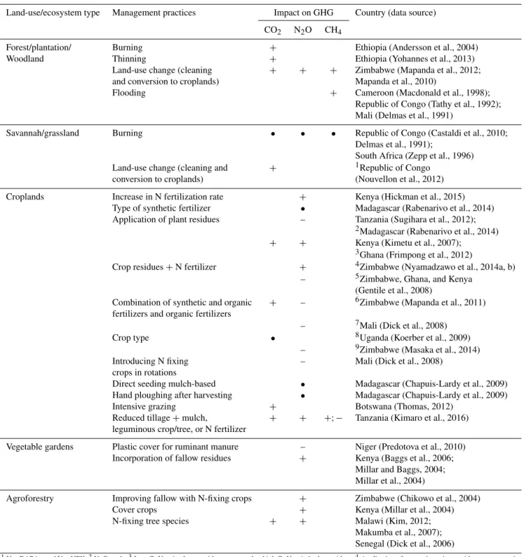
Table 4.Summary of the effect of management practices on greenhouse gas (GHG) emissions.+indicates increasing,•indicates no change, and – indicates decreasing.
Land-use/ecosystem type Management practices Impact on GHG Country (data source)
CO2 N2O CH4
Forest/plantation/ Burning + Ethiopia (Andersson et al., 2004)
Woodland Thinning + Ethiopia (Yohannes et al., 2013)
Land-use change (cleaning + + + Zimbabwe (Mapanda et al., 2012;
and conversion to croplands) Mapanda et al., 2010)
Flooding + Cameroon (Macdonald et al., 1998);
Republic of Congo (Tathy et al., 1992); Mali (Delmas et al., 1991)
Savannah/grassland Burning • • • Republic of Congo (Castaldi et al., 2010;
Delmas et al., 1991);
South Africa (Zepp et al., 1996)
Land-use change (cleaning and + 1Republic of Congo
conversion to croplands) (Nouvellon et al., 2012)
Croplands Increase in N fertilization rate + Kenya (Hickman et al., 2015)
Type of synthetic fertilizer • Madagascar (Rabenarivo et al., 2014)
Application of plant residues – Tanzania (Sugihara et al., 2012);
2Madagascar (Rabenarivo et al., 2014)
+ + Kenya (Kimetu et al., 2007);
3Ghana (Frimpong et al., 2012)
Crop residues+N fertilizer + 4Zimbabwe (Nyamadzawo et al., 2014a, b)
– 5Zimbabwe, Ghana, and Kenya
(Gentile et al., 2008)
Combination of synthetic and organic + – 6Zimbabwe (Mapanda et al., 2011)
fertilizers and organic fertilizers
– 7Mali (Dick et al., 2008)
Crop type • 8Uganda (Koerber et al., 2009)
– 9Zimbabwe (Masaka et al., 2014)
Introducing N fixing – Mali (Dick et al., 2008)
crops in rotations
Direct seeding mulch-based • Madagascar (Chapuis-Lardy et al., 2009)
Hand ploughing after harvesting • Madagascar (Chapuis-Lardy et al., 2009)
Intensive grazing + Botswana (Thomas, 2012)
Reduced tillage+mulch, + + +; − Tanzania (Kimaro et al., 2016)
leguminous crop/tree, or N fertilizer
Vegetable gardens Plastic cover for ruminant manure – Niger (Predotova et al., 2010)
Incorporation of fallow residues + Kenya (Baggs et al., 2006;
Millar and Baggs, 2004; Millar et al., 2004)
Agroforestry Improving fallow with N-fixing crops + Zimbabwe (Chikowo et al., 2004)
Cover crops + Kenya (Millar et al., 2004)
N-fixing tree species + + Malawi (Kim, 2012;
Makumba et al., 2007); Senegal (Dick et al., 2006)
1U+DAP instead U+NPK.2N
2O study.3Low C : N ratio clover residues compared to high C : N ratio barley residues.4Application of ammonium nitrate with manure to maize
(Zea maysL.) and winter wheat (Triticum aestivumL.) plant residues.5Plant residues of maize, calliandra, and tithonia+urea.6Mixed application of composted manure and
inorganic fertilizer (AN).7Manure and urea.8Lettuces vs. cabbages vs. beans.9Tomatoes vs. rape.
efflux also varied with vegetation types (Table 3). For exam-ple, annual soil CO2 emissions were significantly lower in N-fixing acacia monocultures than in eucalypt monocultures and mixed-species stands in the Republic of Congo (Epron et al., 2013). The differences were attributed to leaf area index
that in forests, litterfall accounted for most of the age-related trends after the first year of growth, with litter decomposition producing 44 % of soil CO2flux in the oldest stand (Nouvel-lon et al., 2012), suggesting that the amount and quality of litter plays a major role in determining soil CO2flux. How-ever, the effect of vegetation type can also interact with soil physical–chemical properties. For example, in Benin, root respiration contributed to 30 % of total soil CO2efflux in oil palms when the soil was at field capacity and 80 % when soil was dry (Lamade et al., 1996).
Forest management such as burning, which is a common practice in SSA, and thinning affects GHG emissions (Ta-ble 4). The IPCC Tier 1 methodology only calculates the amount of GHG emissions as a percentage of the carbon that is released through the burning; however, it may also in-crease forest soil GHG emissions once the fire has passed. For example, soil CO2 efflux immediately increased after burning of woodland in Ethiopia (Andersson et al., 2004); also, 5 days after burning, rainfall resulted in a 2-fold in-crease in soil CO2 efflux from the burned plots compared to the unburned plots. In contrast, 12 days after burning soil CO2efflux was 21 % lower in the burned plots (Andersson et al., 2004). However, contrasting impacts of fire on soil GHG emission were observed in a savannah/grassland in the Re-public of Congo, where fire did not change soil CO2, CH4, and N2O fluxes (Castaldi et al., 2010; Delmas et al., 1991). Similarly, in South Africa, soil CH4efflux was not signifi-cantly affected by burning (Zepp et al., 1996). In contrast, annual fires decreased soil CH4oxidation rates in a Ghanaian savannah (Prieme and Christensen, 1999). These case studies demonstrate that fire impacts are not always consistent and this is likely the result of different fire characteristics (e.g., intensity or frequency), soil type (e.g., Kulmala et al., 2014; Kim et al., 2011), and post-fire weather conditions. Thinning forest cover can also increase soil CO2 efflux. Yohannes et al. (2013) reported 24 and 14 % increases in soil CO2efflux in the first and second years following thinning of a 6-year-oldCupressus lusitanicaplantation in Ethiopia.
There is a particular paucity of data on sources and sinks of CH4 in African natural terrestrial systems. In Cameroon, the largest CH4 oxidation rates were observed from relatively undisturbed near-primary forest sites (−14.7 to−15.2 ng m−2s−1)compared to disturbed forests (−10.5 to 0.6 ng m−2s−1; Macdonald et al., 1998). Savannah and grassland were found to be both a sink and a source of CH4. In Mali, CH4 uptake was observed in dry sandy savannah (Delmas et al., 1991), while a savannah in Burkina Faso was found to be both a CH4sink and source during the rainy sea-son, although overall it was a net CH4source (Brümmer et al., 2009). Termite mounds are known sources of CH4and CO2 (Nyamadzawo et al., 2012; Brümmer et al., 2009). A study in a Burkina Faso savannah found that CH4and CO2 released by termites (Cubitermes fungifaber)contributed 8.8 and 0.4 % of total soil CH4and CO2emissions, respectively (Brümmer et al., 2009). In Cameroon, the mounds of
soil-feeding termites (Thoracotermes macrothoraxand
Cubiter-mes fungifaber) were point sources of CH4, which at the
landscape scale may exceed the general sink capacity of the soil (Macdonald et al., 1998). In Zimbabwe, it was found
thatOdontotermes transvaalensistermite mounds located in
dambos (seasonal wetlands) were an important source of GHGs, and emissions varied with catena position for CO2 and CH4(Nyamadzawo et al., 2012).
Compared to the other environments covered in this re-view there are very few studies from salt pans. Thomas et al. (2014), however, found soil CO2 efflux increased with temperature and also increased for a few hours af-ter flooding of the surface of the Makgadikgadi salt pan in Botswana. Annual CO2emissions in salt pan were estimated as 0.7 Mg CO2ha−1yr−1(Thomas et al., 2014).
Aquatic systems
African aquatic systems such as streams, rivers, wetlands, floodplains, reservoirs, lagoons, and lakes can be significant sources of GHG (Tables 1 and S1). Differences in regional setting and hydrology mean that emissions are highly spa-tially and temporally variable, and when combined with the paucity of studies, it is challenging to identify clear control factors (Table 3).
Studies found SSA aquatic systems can be significant sources of GHG emissions. In Ivory Coast, three out of five lagoons were oversaturated in CO2 during all seasons and all were CO2 sources (3.1–16.2 g CO2m−2d−1)due to net ecosystem heterotrophy and inputs of riverine CO2-rich waters (Koné et al., 2009). In the flooded forest zone of the Congo River basin (Republic of Congo) and the Niger River floodplain (Mali), high CH4 emissions (5.16×10²⁰– 6.35×10²²g CH4m−2d−1)were recorded on flooded soils (Tathy et al., 1992; Delmas et al., 1991). In the Nyong River (Cameroon), CO2 emissions (5.5 kg CO2m−2yr−1)were 4 times greater than the flux of dissolved inorganic carbon (Brunet et al., 2009). In the Zambezi River (Zambia), 38 % of the total C in the river is emitted into the atmosphere, mostly as CO2(98 %; Teodoru et al., 2015). The source of CH4to the atmosphere from Lake Kivu corresponded to∼60 % of the terrestrial sink of atmospheric CH4over the lake’s catch-ment (Borges et al., 2011). A recent study of 10 river systems in SSA estimated water–air CO2, CH4, and N2O fluxes to be 8.2 to 66.9 g CO2m−2d−1, 0.008 to 0.46 g CH4m−2d−1, and 0.09 to 1.23 mg N2O m−2d−1, respectively (Borges et al., 2015). The authors suggested that lateral inputs of CO2 from soils, groundwater, and wetlands were the largest con-tributors of the CO2emitted from the river systems (Borges et al., 2015).
(37.9–62.9 g CO2m−2d−1) in the Congo Basin (Mann et al., 2014). The average CH4 flux in river channels (0.75 g CH4m−2d−1) was higher than that in flood-plains and lagoons (0.41–0.49 g CH4m−2d−1) in the Okavango Delta (Botswana; Gondwe and Masamba, 2014). Methane emissions from river deltas were substan-tially higher (∼103 mg CH4m−2d−1) than those from non-river bays (< 100 mg CH4m−2d−1) in Lake Kariba (Zambia/Zimbabwe). Methane fluxes were higher in river deltas (∼103 mg CH4m−2d−1) compared to non-river bays (< 100 mg CH4m−2d−1) in Lake Kariba (Zam-bia/Zimbabwe; DelSontro et al., 2011). While CO2and CH4 concentrations in the main channel were highest downstream of the floodplains, N2O concentrations were lowest down-stream of the floodplains in the Zambezi River (Zambia and Mozambique; Teodoru et al., 2015). Greenhouse gas emissions from Dambos in Zimbabwe varied with catena position (Nyamadzawo et al., 2014a). Upland dambos were important sources of N2O and CO2, and a sink for CH4, while those in a mid-slope position were a major source of CH4 but a weak source of CO2 and N2O, and those at the bottom were a weak source of all GHGs (Nyamadzawo et al., 2014a).
The concentration and flux of GHGs are strongly linked to hydrological characteristics such as discharge (Table 3), but clear patterns have not yet been identified. Surface CO2 flux was positively correlated with discharge in the Congo River (Wang et al., 2013), while in Ivory Coast, rivers were often oversaturated with CO2and the seasonal variability in partial pressure of CO2(pCO2)was due to dilution during the flooding period (Koné et al., 2009). Similarly, CO2fluxes show a very pronounced seasonal pattern strongly linked to hydrological conditions in the Oubangui River in the Central African Republic (Bouillon et al., 2012). Although higher CH4concentrations were found during low-discharge condi-tions, N2O concentrations were lowest during low-discharge conditions (Bouillon et al., 2012). In Lake Kivu, seasonal variations of CH4 in the main basin were driven by deep-ening of the mixolimnion and mixing of surface waters with deeper waters rich in CH4(Borges et al., 2011). In the Zam-bezi River (Zambia and Mozambique), interannual variabil-ity was relatively large for CO2 and CH4 and significantly higher concentrations were measured during wet seasons (Teodoru et al., 2015). However, interannual variability in N2O was less pronounced and generally higher values were found during the dry season (Teodoru et al., 2015). In Kam-pala, Uganda, precipitation was a major driver for seasonal variation of CO2, CH4, and N2O fluxes in subsurface flow wetland buffer strips due to its potential influence on hy-draulic saturation affecting oxygen fluctuation (Bateganya et al., 2015).
Studies found the concentration and flux of GHGs are also strongly linked to environment and water quality (Table 3) but clear patterns have not yet been identified. In the Oka-vango Delta (Botswana), CH4emissions were highest during
the warmer, summer rainy season and lowest during cooler winter season, suggesting the emissions were probably regu-lated by water temperature (Gondwe and Masamba, 2014). However, Borges et al. (2015) found no significant corre-lation between water temperature andpCO2 and dissolved CH4and N2O in 11 SSA river systems, but there was a pos-itive relationship betweenpCO2and dissolved organic C in six of the rivers. They also found the lowest N2O values were observed at the highestpCO2 and lowest % O2 lev-els, suggesting the removal of N2O by denitrification (Borges et al., 2015). In Lake Kivu (East Africa), the magnitude of CO2 emissions to the atmosphere seems to depend mainly on inputs of dissolved inorganic carbon from deep geother-mal springs rather than on the lake metabolism (Borges et al., 2014).
3.2.2 Greenhouse gas emissions from agricultural lands Agricultural GHG emissions in SSA are substantial, amount-ing to 26 % of the continent’s total GHG emissions (Valentini et al., 2014) compared to 8.4 % of total GHG emissions in the USA (US EPA, 2016). Identifying controls on the emission of GHG from SSA agricultural land is challenging because both natural variations associated with climate and soil type and management factors including nutrients (particularly fer-tilization) and crop type affect GHG emissions.
Croplands
The effects of the amount and type of N input on N2O emis-sions in croplands have been studied in several locations (Ta-ble 4). In western Kenya, the rate of N fertilizer application (0 to 200 kg N ha−1)on maize fields had no significant effect on N2O emissions (620 to 710 g N2O–N ha−1 for 99 days; Hickman et al., 2014). However, another study from west-ern Kenya found a relationship between N input and N2O emissions that was best described by an exponential model with the largest impact on N2O emissions occurring when N inputs increased from 100 to 150 kg N ha−1(Hickman et al., 2015). An incubation study in Madagascar demonstrated that application of mixed urea and diammonium phosphate re-sulted in lower N2O emissions (28 vs. 55 ng N2O–N g−1h−1 for 28 days, respectively) than a mixed application of urea and NPK fertilizer (Rabenarivo et al., 2014).
et al., 2014). In contrast, incorporation of Tithonia diver-sifolia (tithonia) leaves led to greater N2O emissions com-pared to urea application in maize fields in Kenya (Sommer et al., 2015; Kimetu et al., 2007). The higher N2O emis-sions after incorporation of Tithonia diversifolia were at-tributed to high levels of nitrate and available carbon in the soil caused by the application that subsequently enhanced denitrification rates. In incubation studies with cultivated soil from Ghana, N2O emissions were significantly higher from soils amended with low C : N ratio clover residues compared to high C : N ratio barley residues (Frimpong et al., 2012). Increasing the proportion of maize in a cowpea– maize residue significantly decreased N2O emissions com-pared to cowpea residue incorporation alone (Frimpong et al., 2011), again likely due to the higher C : N ratio of the maize residue compared with the cowpea. Another incuba-tion study with cultivated soil from Ghana showed that N2O emissions increased after incorporation of residues of three tropical plant species (Vigna unguiculata,Mucuna pruriens,
andLeucaena leucocephala) and emissions were positively
correlated with the C : N ratio of the residue, and nega-tively correlated with residue polyphenol content, polyphe-nol : N ratio and (lignin+polyphenol) : N ratio (Frimpong and Baggs, 2010). It is rare for N2O emissions to be posi-tively correlated with the C : N ratio, and the authors of the study suggest that it was either because soil C was limiting denitrification rates or that release of N from the residues was slow (Frimpong and Baggs, 2010). The results demon-strate that the quality of residues (e.g., C : N ratio, N, lignin, and soluble polyphenol contents) affects GHG emissions and further studies are needed to clearly identify the relationship between them (Snyder et al., 2009; Mafongoya et al., 1997). Adding an additional N (mineral or organic) when crop residues are incorporated into the soil could stimulate min-eralization of crop residues, increase N-use efficiency and produce higher yields (e.g., Garcia-Ruiz and Baggs, 2007; Table 4). It was found that application of mixed crop residue or manure and inorganic fertilizers resulted in different re-sponse of CO2 and N2O emissions. In maize (Zea mays L.) and winter wheat (Triticum aestivumL.) fields in Zim-babwe, application of inorganic fertilizer (ammonium nitrate, NH4NO3-N) with manure increased CO2 emissions (26 to 73 %) compared to sole application of manure (Nyamadzawo et al., 2014a). However, the mixed application resulted in lower yield-scaled N2O emissions (1.6–4.6 g N2O kg−1 yield), compared to sole application of inorganic fertilizer (6–14 g N2O kg−1 yield; Nyamadzawo et al., 2014a). Sim-ilarly, in a maize field in Zimbabwe, N2O emissions were lower after the application of composted manure and inor-ganic fertilizer (NH4NO3-N) compared to sole application of inorganic fertilizer. The same treatments, however, led to the opposite results for CO2emissions (Mapanda et al., 2011). In Mali, pearl millet (Pennisetum glaucum) fields treated with both manure and inorganic fertilizer urea emitted signifi-cantly less N2O than plots receiving only urea fertilizer (Dick
et al., 2008). The lower N2O emissions in soils amended with manure were attributed to the initial slow release and im-mobilization of mineral N and the consequently diminished pool of N available to be lost as N2O (Nyamadzawo et al., 2014a, b; Mapanda et al., 2011; Dick et al., 2008). In an in-cubation study with cultivated soils from Zimbabwe, Ghana, and Kenya, combining organic residue (maize, calliandra, and tithonia) and urea fertilizers decreased N2O emissions in coarse-textured soils but increased N2O emissions in fine-textured soils due to the higher level of available N (Gentile et al., 2008).
Grazing grassland
We only found two studies reporting GHG emissions in pas-toral grasslands, and there remains a serious gap in our under-standing of GHG emissions in these systems. Thomas (2012) found that soil CO2efflux from a Botswana grazing land was significantly higher in sandy soils where the biological soil crust (BSC) was removed and on calcrete where the BSC was buried under sand. The results indicated the importance of BSCs for C cycling in drylands and intensive grazing, which destroys BSCs through trampling and burial, will adversely affect C sequestration and storage (Thomas, 2012). Rosen-stock et al. (2016) measured GHG fluxes from two pastures in western Kenya and found that CO2emissions ranged from 13.4 to 15.9 Mg CO2ha−1yr−1, similar to levels found in the Amazon (Davidson et al., 2000).
Rice paddies
Rice paddies are well-known sources of CH4(e.g., Linquist et al., 2012). Experiments measuring GHG emissions in rice paddies have been conducted in Kenya (Tyler et al., 1988) and Zimbabwe (Nyamadzawo et al., 2013). In Kenya, CH4 fluxes did not show any seasonal trend and did not indicate appreciable variability among two different strains of rice (Tyler et al., 1988). In Zimbabwe, intermittently saturated dambo rice paddies were a source of GHG and annual emissions (150-day growing season and 126 kg of applied N ha−1) were estimated as 2.7 Mg CO
2ha−1yr−1, 12.5 kg CH4ha−1, and 0.12 kg N2O ha−1 (Nyamadzawo et al., 2013). The IPCC (2006) uses a CH4 emission factor of 1.30 kg CH4ha−1day−1 for rice cultivation. The CH4 emissions in the dambo rice paddies re-ferred to here are much lower than the IPCC estimate (195 kg CH4ha−1=1.3 kg CH4ha−1day−1×150 days). The corresponding IPCC (2006) N2O EF is 0.3 % for rice cultivation, and thus the N2O emissions in the dambo rice paddies are also much lower than the IPCC esti-mate (0.40 kg N2O−N ha−1=126 kg N ha−1×0.003; 0.63 kg N2O ha−1). These results suggest the potential for large deviations from expected emissions based on existing information.
Vegetable gardens
Greenhouse gas emissions from soils in vegetable gar-dens in peri-urban areas of Burkina Faso (Lompo et al., 2012) and Niger (Predotova et al., 2010) ranged from 73.3 to 132.0 Mg CO2ha−1yr−1 and 53.4 to 177.6 kg N2O ha−1yr−1(Tables 1 and S1).
In Burkina Faso, annual CO2 and N2O emissions from vegetable garden soils were 68 to 85 and 3 to 4 % of total C and N input, respectively (Lompo et al., 2012). The N2O EFs (3 to 4 %) were higher than the IPCC default value of 1.0 % for all cropping systems (IPCC, 2006) and the global
N2O EF of vegetable fields (0.94 %; Rezaei Rashti et al., 2015). The high N2O EFs may be attributed to the exces-sive amount of applied N (2700–2800 kg N ha−1yr−1)to get high yields in vegetable gardens since surplus N will stimu-late N2O production and inhibit biochemical N2O reduction (e.g., Shcherbak et al., 2014; Kim et al., 2013). In vegetable gardens of Niger, a simple plastic sheet roofing and addi-tion of ground rock phosphate to stored ruminant manure de-creased N2O gaseous losses by 50 % in comparison to dung directly exposed to the sun (Predotova et al., 2010).
Agroforestry
Soil CO2and N2O emissions from African agroforestry were 38.6 Mg CO2ha−1yr−1 and 0.2 to 26.7 kg N2O ha−1yr−1, respectively (Tables 1 and S1).
Improving fallow with N-fixing trees is a common agro-forestry practice in several areas of Africa since it provides additional N to the soil that can be utilized by the subsequent cash crop (e.g., Makumba et al., 2007; Chikowo et al., 2004; Dick et al., 2001). However, the practice is also thought to increase CO2and N2O emissions compared to conventional croplands (Table 4). Nitrous oxide emissions increased after incorporation of fallow residues and emissions were higher after incorporation of improved-fallow legume residues than natural-fallow residues (Baggs et al., 2006; Millar and Baggs, 2004; Millar et al., 2004). It was found that N2O emissions were positively correlated with residue N content (Baggs et al., 2006; Millar et al., 2004) and negatively correlated with polyphenol content and its protein binding capacity (Millar and Baggs, 2004), soluble C-to-N ratio (Millar and Baggs, 2005), and lignin content (Baggs et al., 2006). While high residue N content likely leads to more available soil N and consequently increased N2O production (Baggs et al., 2006; Millar and Baggs, 2005; Millar et al., 2004), polyphenols and lignins are both resistant to decomposition and could result in N immobilization resulting in less labile soil N and less N2O production (Baggs et al., 2006; Millar and Baggs, 2004). Therefore, there may be potential to reduce N2O emissions from agroforestry, but it may require ecological nutrient man-agement (i.e., reduced inorganic fertilizer N inputs, account-ing for N input from the legume trees; addaccount-ing a C source such as a cover crop together with an N source) and rotation planning.
As in natural systems, N2O emissions from agroforestry are also affected by rainfall events. In an incubation exper-iment in Uganda, N2O emissions following simulated rain-fall were at least 4 times larger for soils from under N-fixing trees (Calliandra calothyrsus) compared to soils with non-N fixing trees (Grevillea robusta; Dick et al., 2001). Simi-larly, in Mali, N2O emissions were around 6 times higher from improved fallow with N-fixing trees (Gliricidia sepium
home gardens in Sudan, CO2and N2O fluxes were positively correlated with soil moisture (Goenster et al., 2015).
3.2.3 Greenhouse gas emissions from land-use change Land-use change has been recognized as the largest source of GHG emission in Africa (Valentini et al., 2014). Conver-sion rates of African natural lands, including forest, grassland and wetland, to agricultural lands have increased in recent years (Gibbs et al., 2010; FAO, 2010). The dominant type of land-use change has been the conversion of forest to agricul-ture with average deforestation rates of 3.4 Mha yr−1 (FAO-STAT, 2014; Fig. 1). This land-use conversion results in an estimated additional release of 0.32±0.05×10⁹Mg C yr−1 (Valentini et al., 2014) or 157.9±23.9×10⁹Mg CO2eq. in 1765 to 2005 (Kim and Kirschbaum, 2015), higher than fos-sil fuel emissions for Africa (Valentini et al., 2014). Land-use change affects soil GHG emissions due to changes in vege-tation, soil, hydrology, and nutrient management (e.g., Kim and Kirschbaum, 2015) and the effects of land-use change on soil GHG emissions have been observed in African wood-lands and savannah. Clearing and converting woodwood-lands to croplands increased soil emissions of CO2, CH4, and N2O (Mapanda et al., 2012), and soil CO2 emissions from the converted croplands were higher thanEucalyptusplantations established in former natural woodlands (Mapanda et al., 2010). Changes in soil CO2 efflux after afforestation of a tropical savannah withEucalyptuswere mostly driven by the rapid decomposition of savannah residues and the increase in
Eucalyptusrhizospheric respiration (Nouvellon et al., 2012).
3.3 Suggested future research
Despite an increasing number of published estimates of GHG emissions in the last decade, there remains a high degree of uncertainty about the contribution of AFOLU to emissions in SSA (Table 5). To address this and reduce the uncertainty surrounding the estimates, additional GHG emission mea-surements that fully capture seasonal and annual variations across natural ecosystems and agricultural lands throughout SSA are urgently required. Identifying controlling factors and their effects on GHG fluxes is a pre-requisite to enhanc-ing our understandenhanc-ing of efflux mechanisms and a necessary step towards scaling up the field-scale data to landscape, na-tional, and continental scales (Table 5). It is important to know how GHG fluxes can be affected by management prac-tices and natural events such as logging (e.g., Yashiro et al., 2008), thinning (e.g., Yohannes et al., 2013), storms (e.g., Vargas, 2012), pest outbreaks (e.g., Reed et al., 2014), fires (e.g., Andersson et al., 2004), and woody shrub encroach-ment (e.g., Smith and Johnson, 2004) in natural terrestrial systems and changing discharge (e.g., Wang et al., 2013) and water table (e.g., Yang et al., 2013) in aquatic systems. It is also important in agricultural lands to know how GHG fluxes are affected by management factors such as soil compaction
(e.g., Ball et al., 1999), tillage (e.g., Sheehy et al., 2013), removal of crop residues (Jin et al., 2014), incorporation of crop residues and synthetic fertilizer (e.g., Nyamadzawo et al., 2014a), N input (whether organic or inorganic; e.g., Hick-man et al., 2015), and crop type (e.g., Masaka et al., 2014). However, because management and soil physical–chemical interactions cause different responses in soil GHG emissions (e.g., Pelster et al., 2012), it is critical to measure these inter-action effects in the African context. The effect of predicted climatic change in Africa such as increased temperature (e.g., Dijkstra et al., 2012), changing rainfall patterns (e.g., Hall et al., 2006), increase in droughts incidence (e.g., Berger et al., 2013), rewetting effects (e.g., Kim et al., 2012b), and increased atmospheric CO2concentration (e.g., Lane et al., 2013) also require further testing using laboratory and field experiments. Future research should consider the wider GHG budget of agriculture and include all the various (non-soil) components such as fuel use, as well as embodied emissions in chemical inputs.
Where possible, studies should seek to identify and sepa-rate the processes contributing to efflux of soil CO2(e.g., au-totrophic and heterotrophic sources), CH4(e.g., methanogen-esis and methanotrophy), and N2O (e.g., nitrification, denitri-fication, and nitrifier denitrification) and link new knowledge of microbial communities (e.g., functional gene abundance) to GHG emissions rates. This is important because the conse-quences of increasing GHG emissions depend on the mech-anism responsible. For example, if greater soil CO2 efflux is primarily due to autotrophic respiration from plant roots, then it simply reflects greater plant growth. If, however, it is due to heterotrophic microbial respiration of soil organic car-bon, then it represents a depletion of soil organic matter and a net transfer of C from soil to the atmosphere. Currently, there are very few studies that differentiate these sources, making it impossible to truly determine the consequences and impli-cations on changes in soil GHG efflux.
Land-use change has been recognized as the largest source of GHG emission in Africa (Valentini et al., 2014). Hence, various types of conversion from natural lands to different land-use types should be assessed to know how these changes may affect the GHG budget (e.g., Kim and Kirschbaum, 2015). The focus of the assessment should be on deforesta-tion and wetland drainage, followed by a conversion to agri-cultural lands, since they are dominant types of land-use change in Africa (Valentini et al., 2014).
Table 5.Summary of status of knowledge of greenhouse gas emission processes, control factors, estimation, and model prediction.
CO2 N2O CH4
Processes & Annual flux Model Processes & Annual flux Model Processes & Annual flux Model control factors estimate prediction control factors estimate prediction control factors estimate prediction
Forest/plantation/woodland 1 2 4 3 3 4 3 3 4
Savannah 2 3 4 3 4 4 3 4 4
Aquatic systems 2 3 4 3 3 4 2 3 4
Cropland 2 3 4 2 2 4 3 4 4
Agroforestry 3 4 4 2 3 4 4 4 4
Vegetable gardens 3 4 4 3 4 4 4 4 4
Rice field 3 4 4 3 4 4 4 4 4
Grazing grassland 3 4 4 4 4 4 4 4 4
1: Robust knowledge – incremental work needed. 2: Existing knowledge base – coordinated work needed. 3: A growing knowledge base – with many gaps and comprehensive work still needed. 4: Emerging knowledge base – significant research effort required.
3.4 Strategic approaches for data acquisition
A strategic plan for acquisition of soil GHG emission data in sub-Saharan Africa is required. The success of any plan is dependent on long-term investment, stakeholder involve-ment, technical skill, and supporting industries, which have not always been available in the region (Olander et al., 2013; Franks and Hadingham, 2012). A major challenge is to address the lack of consistency in the various method-ologies used to quantify GHG emissions (Rosenstock et al., 2013). Relatively low cost and simple techniques can be used to determine GHG emission estimates in the first instance. Soil CO2fluxes can be quantified with a soda lime method (Tufekcioglu et al., 2001; Cropper et al., 1985; Edwards, 1982) or an infrared gas analyzer (Bastviken et al., 2015; Verchot et al., 2008; Lee and Jose, 2003), and these do not require advanced technology or high levels of resource to undertake. Later, other GHG such as N2O and CH4fluxes in addition to CO2flux can be measured with more advanced technology (e.g., gas chromatography, photoacoustic spec-troscopy, or laser gas analyzers). Initially, the measurement can be conducted using manual gas chambers with periodi-cal sampling frequencies. The sampling interval can be de-signed so that it is appropriate to the particular type of land use or ecosystem, management practices, and/or for captur-ing the effects of episodic events (e.g., Parkin, 2008). For ex-ample, GHG measurement should be more during potentially high GHG emission periods following tillage and fertilizer applications and rewetting by natural rainfalls or irrigation. With more advanced technology and utilization of automatic chamber systems, measurements can be conducted at a much higher frequency with relative ease.
In order for the challenges associated with improving our understanding of GHG emissions from African soils, it is critical to establish networks of scientists and scientific bod-ies both within Africa and across the world. Good commu-nication and collaboration between field researchers and the modeling community should also be established during the initial stages of research, so results obtained from field sci-entists can be effectively used for model development and to
generate hypotheses to be tested in the field and laboratory (de Bruijn et al., 2009).
Furthermore, lessons learned from scientific experiments can only really be successfully implemented by farmers if local stakeholders are involved from the start and throughout (see, for example, Stringer et al., 2012). Interviews, focus-groups, on-site or farm demonstrations, local capacity build-ing trainbuild-ing, local farmers, and extension staff can all im-prove dialogue and understanding between local communi-ties and scientists, ultimately improving the likelihood of successful GHG emission and mitigation strategies. These will equip local researchers and stakeholders (including farmers and extension staff) with state-of-the-art methodolo-gies and help motivate them to develop their GHG mitiga-tion measures and assist them in understanding their roles and contributions to global environmental issues. Moreover, data acquisition will be determined not only by technical but also by sociopolitical (and economic) barriers in sub-Saharan Africa. These problems not only affect data acquisition but are also the driving forces for GHG emissions due to land-use change events.
4 Conclusions
data gap. The strategy needs to involve identifying priorities for data acquisition, utilizing appropriate technologies, and establishing networks and collaboration.
5 Data availability
We have created a blog entitled “Greenhouse gas emissions in Africa: study summary and database” (http://ghginafrica. blogspot.com/) and an open-access database, which can be modified by the users, entitled “Soil greenhouse gas emis-sions in Africa database” (linked in the blog) based on this review. In the blog, we have posted a technical summary of each section of this review, where comments can be left un-der the posts. The database contains detailed information on the studies reported on GHG emissions, such as ecosystem and land-use types, location, climate, vegetation type, crop type, fertilizer type, N input rate, soil properties, GHGs emis-sion measurement periods, N2O EF, and corresponding refer-ence. The database is hosted in web-based spreadsheets and is easily accessible and modified. The authors do not have any relationship with the companies currently being used to host the blog or databases.
The Supplement related to this article is available online at doi:10.5194/bg-13-4789-2016-supplement.
Acknowledgements. We are grateful for the numerous researchers and technicians who provided invaluable data. It is impossible to cite all the references due to limited space allowed and we apologize for the authors whose work has not been cited. We are also grateful to Benjamin Bond-Lamberty and Rodrigo Vargas for insightful comments, Luis Lassaletta for guiding us with N applica-tion rates in Africa, and Antony Smith for creating maps showing study sites. Alberto Sanz-Cobena gratefully acknowledges the Spanish Ministry of Science and Innovation and the Autonomous Community of Madrid for their economic support through the NEREA project ( C05-01, AGL2012-37815-C05-04), the Agrisost Project (S2013/ABI-2717), and the FACCE JPI MACSUR project. Dong-Gill Kim acknowledges support from Research and Development Office, Wondo Genet College, and the IAEA Coordinated Research Project (CRP D1 50.16). David Pelster and Todd S. Rosenstock would like to thank the CGIAR Research Program on Climate Change, Agriculture, and Food Security and its Standard Assessment of Mitigation Potential and Livelihoods in Smallholder Systems (SAMPLES) Programme for technical and financial support.
Edited by: M. Weintraub
Reviewed by: three anonymous referees
References
Andersson, M., Michelsen, A., Jensen, M., and Kjøller, A.: Tropi-cal savannah woodland: Effects of experimental fire on soil mi-croorganisms and soil emissions of carbon dioxide, Soil Biol. Biochem., 36, 849–858, 2004.
Baggs, E., Chebii, J., and Ndufa, J.: A short-term investigation of trace gas emissions following tillage and no-tillage of agro-forestry residues in western Kenya, Soil Till. Res., 90, 69–76, 2006.
Ball, B. C., Scott, A., and Parker, J. P.: Field N2O, CO2and CH4
fluxes in relation to tillage, compaction and soil quality in Scot-land, Soil Till. Res., 53, 29–39, 1999.
Barton, L., Wolf, B., Rowlings, D., Scheer, C., Kiese, R., Grace, P., Stefanova, K., and Butterbach-Bahl, K.: Sampling frequency affects estimates of annual nitrous oxide fluxes, Sci. Rep., 5, 15912, doi:10.1038/srep15912, 2015.
Bastviken, D., Sundgren, I., Natchimuthu, S., Reyier, H., and Gål-falk, M.: Technical Note: Cost-efficient approaches to measure carbon dioxide (CO2) fluxes and concentrations in terrestrial and
aquatic environments using mini loggers, Biogeosciences, 12, 3849–3859, doi:10.5194/bg-12-3849-2015, 2015.
Bateganya, N. L., Mentler, A., Langergraber, G., Busulwa, H., and Hein, T.: Carbon and nitrogen gaseous fluxes from subsurface flow wetland buffer strips at mesocosm scale in east Africa, Ecol. Eng., 85, 173–184, 2015.
Berger, S., Jung, E., Köpp, J., Kang, H., and Gebauer, G.: Mon-soon rains, drought periods and soil texture as drivers of soil N2O fluxes – Soil drought turns East Asian temperate deciduous for-est soils into temporary and unexpectedly persistent N2O sinks,
Soil Biol. Biochem., 57, 273–281, 2013.
Birch, H. F.: Mineralisation of plant nitrogen following alternate wet and dry conditions, Plant Soil, 20, 43–49, 1964.
Bombelli, A., Henry, M., Castaldi, S., Adu-Bredu, S., Arneth, A., de Grandcourt, A., Grieco, E., Kutsch, W. L., Lehsten, V., Rasile, A., Reichstein, M., Tansey, K., Weber, U., and Valentini, R.: An outlook on the Sub-Saharan Africa carbon balance, Biogeo-sciences, 6, 2193–2205, doi:10.5194/bg-6-2193-2009, 2009. Bond-Lamberty, B. and Thomson, A. M.: Temperature-associated
increases in the global soil respiration record, Nature, 464, 579– 582, 2010.
Borges, A. V., Abril, G., Delille, B., Descy, J.P., and Darcham-beau, F.: Diffusive methane emissions to the atmosphere from Lake Kivu (Eastern Africa), J. Geophys. Res, 116, G03032, doi:10.1029/2011JG001673, 2011.
Borges, A. V., Morana, C., Bouillon. S., Servais, P., Descy, J.-P., and Darchambeau, F.: Carbon cycling of Lake Kivu (East Africa):
net autotrophy in the epilimnion and emission of CO2to the
at-mosphere sustained by geogenic inputs, PLoS one, 9, e109500, doi:10.1371/journal.pone.0109500, 2014.
Borges, A. V., Darchambeau, F., Teodoru, C. R., Marwick, T. R., Tamooh, F., Geeraert, N., Omengo, F. O., Guerin, F., Lambert, T., Morana, C., Okuku, E., and Bouillon, S.: Globally signifi-cant greenhouse-gas emissions from African inland waters, Nat. Geosci., 8, 637–642, doi:10.1038/ngeo2486, 2015.
Bouwman, A. F., Beusen, A. H. W., and Billen, G.: Human alter-ation of the global nitrogen and phosphorus soil balances for the period 1970–2050, Global Biogeochem. Cy., 23, GB0A04, doi:10.1029/2009GB003576, 2009.
Bouwman, L., Goldewijk, K. K., Van Der Hoek, K. W., Beusen, A. H. W., Van Vuuren, D. P., Willems, J., Rufino, M. C., and Ste-hfest, E.: Exploring global changes in nitrogen and phosphorus cycles in agriculture induced by livestock production over the 1900–2050 period, P. Natl. Acad. Sci. USA, 110, 20882–20887, doi:10.1073/pnas.1012878108, 2013.
Brümmer, C., Papen, H., Wassmann, R., and Brüggemann, N.:
Fluxes of CH4and CO2from soil and termite mounds in south
Sudanian savanna of Burkina Faso (West Africa), Global Bio-geochem. Cy., 23, GB1001, doi:10.1029/2008GB003237, 2009. Brunet, F., Dubois, K., Veizer, J., Nkoue Ndondo, G. R., Ndam Ngoupayou, J. R., Boeglin, J. L., and Probst, J. L.: Terrestrial and fluvial carbon fluxes in a tropical watershed: Nyong basin, Cameroun, Chem. Geol., 2, 563–572, 2009.
Caquet, B., De Grandcourt, A., Thongo M’bou, A., Epron, D., Ki-nana, A., Saint André, L., and Nouvellon, Y.: Soil carbon balance in a tropical grassland: Estimation of soil respiration and its par-titioning using a semi-empirical model, Agr. Forest. Meteorol., 158–159, 71–79, 2012.
Castaldi, S., de Grandcourt, A., Rasile, A., Skiba, U., and Valentini, R.: CO2, CH4and N2O fluxes from soil of a burned grassland in
Central Africa, Biogeosciences, 7, 3459–3471, doi:10.5194/bg-7-3459-2010, 2010.
Chapuis-Lardy, L., Metay, A., Martinet, M., Rabenarivo, M., Toucet, J., Douzet, J. M., Razafimbelo, T., Rabeharisoa, L., and Rakotoarisoa, J.: Nitrous oxide fluxes from malagasy agricultural soils, Geoderma, 148, 421–427, 2009.
Chikowo, R., Mapfumo, P., Nyamugafata, P., and Giller, K. E.: Min-eral n dynamics, leaching and nitrous oxide losses under maize following two-year improved fallows on a sandy loam soil in Zimbabwe, Plant Soil, 259, 315–330, 2004.
Ciais, P., Bombelli, A., Williams, M., Piao, S. L., Chave, J., Ryan, C. M., Henry, M., Brender, P., and Valentini, R.: The Carbon Bal-ance of Africa: Synthesis of Recent Research Studies, Philos. T. R. Soc. A, 269, 2038–2057, 2011.
Cropper Jr., W., Ewel, K.C., and Raich, J.: The measurement of soil
CO2evolution in situ, Pedobiologia, 28, 35–40, 1985.
Davidson, E. A., Verchot, L. V., Cattanio, J. H., Ackerman, I. L., and Carvalho, J.: Effects of soil water content on soil respiration in forests and cattle pastures of eastern Amazonia, Biogeochem-istry, 48, 53–69, 2000.
de Bruijn, A. M. G., Butterbach-Bahl, K., Blagodatsky, S., and Grote, R.: Model evaluation of different mechanisms driving
freeze-thaw N2O emissions, Agric. Ecosyst. Environ., 133, 196–
207, 2009.
Delmas, R. A., Marenco, A., Tathy, J. P., Cros, B., and Baudet, J.
G. R.: Sources and sinks of methane in African savanna. CH4
emissions from biomass burning, J. Geophys. Res., 96, 7287– 7299, 1991.
DelSontro, T., Kunz, M. J., Kempter, T., Wüest, A., Wehrli, B., and Senn, D. B.: Spatial heterogeneity of methane ebullition in a large tropical reservoir, Environ. Sci. Technol., 45, 9866–9873, doi:10.1021/es2005545, 2011.
Díaz-Pinés, E., Schindlbacher, A., Godino, M., Kitzler, B., Jandl, R., Zechmeister-Boltenstern, S., and Rubio, A.: Effects of tree
species composition on the CO2and N2O efflux of a
Mediter-ranean mountain forest soil, Plant Soil, 384, 243–257, 2014. Dick, J., Skiba, U., and Wilson J.: The effect of rainfall on NO and
N2O emissions from Ugandan agroforest soils, Phyton, 41, 73–
80, 2001.
Dick, J., Skiba, U., Munro, R., and Deans, D.: Effect of N-fixing
and non n-fixing trees and crops on NO and N2O emissions from
Senegalese soils, J. Biogeogr., 33, 416–423, 2006.
Dick, J., Kaya, B., Soutoura, M., Skiba, U., Smith, R., Niang, A., and Tabo, R.: The contribution of agricultural practices to nitrous oxide emissions in semi-arid Mali, Soil Use Manage., 24, 292– 301, 2008.
Dijkstra, F. A., Prior, S. A., Runion, G. B., Torbert, H. A., Tian, H., Lu, C., and Venterea, R. T.: Effects of elevated carbon dioxide and increased temperature on methane and nitrous oxide fluxes: evidence from field experiments, Front. Ecol. Environ., 10, 520– 527, 2012.
Dutaur, L. and Verchot, L. V.: A global inventory of the
soil CH4 sink, Global Biogeoche. Cy., 21, GB4013,
doi:10.1029/2006gb002734, 2007.
Edwards, N.: The use of soda-lime for measuring respiration rates in terrestrial systems, Pedobiologia, 23, 321–330, 1982. Epron, D., Nouvellon, Y., Roupsard, O., Mouvondy, W., Mabiala,
A., Saint-André, L., Joffre, R., Jourdan, C., Bonnefond, J.-M., Berbigier, P., and Hamel, O.: Spatial and temporal variations of soil respiration in a eucalyptus plantation in Congo, Forest Ecol. Manage., 202, 149–160, 2004.
Epron, D., Nouvellon, Y., Mareschal, L., e Moreira, R. M., Koutika, L.-S., Geneste, B., Delgado-Rojas, J. S., Laclau, J.-P., Sola, G., and de Moraes Goncalves, J. L.: Partitioning of net primary pro-duction in eucalyptus and acacia stands and in mixed-species plantations: Two case-studies in contrasting tropical environ-ments, Forest Ecol. Manage., 301, 102–111, 2013.
Fan, Z., Neff, J. C., and Hanan, N. P.: Modeling pulsed soil respi-ration in an African savanna ecosystem, Agr. Forest. Meteorol., 200, 282–292, 2015.
FAO: Global Forest Resources Assessment 2010, FAO Forestry Pa-per 163, Food and Agriculture Organization of the United Na-tions, Rome, 340 pp., available at: http://www.fao.org/forestry/ fra/fra2010/en/ (last access: 1 October 2015), 2010.
FAOSTAT: Food and agriculture organization of the United Na-tions, http://faostat.fao.org/site/377/default.aspx#ancor, last ac-cess: 1 October 2015.
Franks, J. R. and Hadingham, B.: Reducing greenhouse gas emis-sions from agriculture: Avoiding trivial solutions to a global problem, Land Use Policy, 29, 727–736, 2012.
Frimpong, K. A. and Baggs, E. M.: Do combined applications of
crop residues and inorganic fertilizer lower emission of N2O
from soil?, Soil Use Manage., 26, 412–424, 2010.
Frimpong, K. A., Yawson, D. O., Baggs, E. M., and Agyarko, K.: Does incorporation of cowpea-maize residue mixes influence ni-trous oxide emission and mineral nitrogen release in a tropical luvisol?, Nutr. Cycl. Agroecosys., 91, 281–292, 2011.
Frimpong, K. A., Yawson, D. O., Agyarko, K., and Baggs, E. M.: N2O emission and mineral N release in a tropical acrisol