www.ann-geophys.net/26/1653/2008/ © European Geosciences Union 2008
Annales
Geophysicae
Alfv´en ship waves: high-
m
ULF pulsations in the magnetosphere
generated by a moving plasma inhomogeneity
P. N. Mager and D. Yu. Klimushkin
Institute of Solar-Terrestrial Physics (ISTP), Russian Academy of Science, Siberian Branch, Irkutsk, P.O. Box 291, 664033, Russia
Received: 8 October 2007 – Revised: 15 February 2008 – Accepted: 18 April 2008 – Published: 11 June 2008
Abstract. The generation of a high-mAlfv´en wave by sub-storm injected energetic particles in the magnetosphere is studied. The wave is supposed to be emitted by an alternating current created by the drifting particle cloud or ring current inhomogeneity. It is shown that the wave appears in some azimuthal location simultaneously with the particle cloud ar-rival at the same spot. The value of the azimuthal wave number is determined asm∼ω/ωd, whereω is the
eigen-frequency of the standing Alfv´en wave andωdis the particle
drift frequency. The wave propagates westward, in the di-rection of the proton drift. Under the reasonable assumption about the density of the energetic particles, the amplitude of the generated wave is close to the observed amplitudes of poloidal ULF pulsations.
Keywords. Magnetospheric physics (MHD waves and in-stabilities) – Space plasma physics (Kinetic and MHD the-ory)
1 Introduction
Alfv´en waves in the range of Pc3–5 can be categorized into the waves with large and small azimuthal wave numbersm. Recently, the high-mwaves were observed with CLUSTER (Eriksson et al., 2005, 2006; Sch¨afer et al., 2007) and radars (Fenrich et al., 1995; Yeoman et al., 2000; Wright et al., 2001; Baddeley et al., 2002). The low-mwaves are generated by the resonant interaction with the fast mode, propagating from the outer boundary of the magnetosphere. This gen-eration mechanism is ineffective for pulsations withm≫1 (azimuthally small scale waves), because in this case only an exponentially small part of the fast mode energy pen-etrates into the magnetosphere (Glassmeier, 1995). Thus, other sources of the wave energy must be found. Substorm
Correspondence to:P. N. Mager ([email protected])
injected protons, drifting in the magnetosphere, appear to be good candidates. It is usually assumed that high-mwaves are excited by unstable proton populations with energies from 10 to 150 keV by means of the drift-bounce instability (Karp-man et al., 1977). An example of this unstable distribution function is the bump-on-tail distribution.
There are a number of arguments to support this sugges-tion. One of them is the coincidence of the directions of the azimuthal phase velocity of the high-mpulsations and the proton drift velocity (Fenrich et al., 1995; Yeoman et al., 2000; Baddeley et al., 2005b; Glassmeier, 1980). Be-sides, both velocities depend on the radial coordinate almost in the same way (Allan et al., 1982, 1983). There is some ev-idence of statistical relations between the high-mpulsations and ring current intensifications (Anderson, 1993; Yeoman et al., 2000). Association of the high-mwaves with nonmono-tonic particle distributions have been observed by Hughes et al. (1978), Glassmeier et al. (1999), Wright et al. (2001) and statistically studied by Baddeley et al. (2002, 2004, 2005a,b). The bump-on-tail distribution is usually supposed to be a result of a substorm injection: faster protons reach a given point on the azimuthal coordinate earlier than lower en-ergy ones, so high-enen-ergy particles are added to the local background plasma at a higher rate than low-energy parti-cles (Karpman et al., 1977; Glassmeier et al., 1999). In-deed, several cases were observed when the wave appeared in some azimuthal location simultaneously with the cloud of the particle injected during substorm arrival in the same spot (Chisham et al., 1992; Wright et al., 2001).
considered by Zolotukhina (1974) and Guglielmi and Zolo-tukhina (1980). A similar problem has been considered for the magnetosphere of Jupiter, where its moon Io acts as the moving wave emitter (Neubauer, 1980). This mechanism re-sembles the generation of waves on the water surface by a moving ship (the analogy of whistlers and a ship wave has been considered by Gurnett, 1995).
Then, the drift-bounce instability does not explain some essential features of the high-m waves. Thus, observed waves have definitemnumbers, although the weekly growth rate depends on this value (Mager and Klimushkin, 2005). Consequently, this instability cannot select a narrow range of themnumbers, contrary to observations. Even the direction of the azimuthal phase velocity of the observed waves cannot be explained: the instability can generate the waves propa-gating in both azimuthal directions (Mager and Klimushkin, 2005). Finally, owing to transformation of poloidal Alfv´en waves into toroidal ones, the instability will be favorable for amplification of toroidal rather than poloidal oscillations (Klimushkin, 2000, 2007; Klimushkin and Mager, 2004). Additional hints that some of the observed high-m pulsa-tions have been generated by nonstationary current are also reported by Pilipenko et al. (2001).
Our paper studies this generation mechanism in the Earth’s magnetosphere. In contrast to the previous efforts in this direction (Akhiezer et al., 1967, 1975; Zolotukhina, 1974; Guglielmi and Zolotukhina, 1980; Neubauer, 1980; Pilipenko et al., 2001), where only a uniform background was considered, we explore a two-dimensionally inhomoge-neous model of the magnetosphere with plasma and mag-netic field non-uniformity along and across with field lines taken into account. Besides, as opposed to some earlier pa-pers (Zolotukhina, 1974; Neubauer, 1980), the field lines are considered to intersect the highly conductive ionospheric plasma, which results in the emergence of a standing wave structure along the field lines. In contrast to our previous pa-per (Mager and Klimushkin, 2007), here we incorporated the dependence of the drift velocity on the radial coordinate: this velocity is supposed to grow with the L-shell.
2 Formulation of the problem
The method for setting up a problem is as follows. At some initial time instantt=0 a cloud of particles is injected into the magnetosphere. The particles are drifting in the azimuthal direction. It is required to obtain an expression for the wave amplitude and to find the spatio-temporal structure and po-larization of the wave field.
The magnetosphere is considered as axially-symmetric and bounded by the highly conductive ionosphere of the Southern and Northern Hemispheres. The cloud of the in-jected particles is assumed to be narrowly localized in az-imuth but distributed over the entire range of L-shells, i.e. in the radial direction. The source is also distributed along field
lines between conjugated points of the ionosphere. Zolo-tukhina (1974) and Neubauer (1980) considered the source compact (localized) in all directions.
The drift angular velocityωd is assumed to be much less
than the characteristic Alfv´en eigenfrequency. In particular, it means that the velocity of the source is much less than the Alfv´en speed. It corresponds to the energies of the order of several tens of keV.
Besides, we assumed the drift angular velocityωd to
in-crease with the radial coordinate (L-shell). For simplicity, we even putωd to be proportional to the radial coordinate,
but we suppose that our results are generally valid for any increasing functionsωd(L). The most common instance is
probably the case when the angular drift speed decreases with the L-shell, because in this case the injected protons conserve the first adiabatic invariant. But, as we will show in the last section, the case considered in the present paper happens to be more interesting, since it shows a rather un-expected feature of the wave field temporal evolution, which can be used for the verification of our model. On the other hand, this case can also be realized in the magnetosphere un-der some conditions (e.g. Southwood, 1980), when there is loss of injected protons. The case when injected protons have a drift velocity constant with radius has been considered in our earlier paper (Mager and Klimushkin, 2007).
Our approach is based on the theory of eigenoscillations of the axisymmetric magnetosphere developed by Leonovich and Mazur (1997) and Klimushkin et al. (2004) and uses the general approach by Akhiezer et al. (1967) and Akhiezer et al. (1975). A time-dependent external current (formed by the moving charged particle cloud) is assumed to be the source term of the wave equation. The particle density of the cloud is considered to be small compared to the background den-sity, which allows us to consider the waves in the linear ap-proximation. The current (wave generator) is considered to be given, that is we neglect the feedback of the generated wave on the current. This assumption is probably valid at the earlier stages of the wave field evolution (Akhiezer et al., 1967). On the other hand, we do not consider the evolution within the first few bounce periods, when the cloud is contin-uing to spread along the field lines and the parallel structure of the wave has not been settled yet. This time is very short because the drift velocity is much less than the thermal par-ticle velocity, so this limitation is not too severe.
3 Main equations
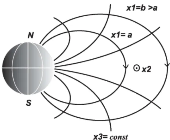
are the coordinate surfacesx1=const (Fig. 1). The coordi-natesx1andx2have the role of the radial and azimuthal co-ordinates, and to represent them we shall use the McIlwain parameterL and the azimuthal angleϕ, respectively. It is convenient to choose a direction of the azimuthal coordinate coinciding with the proton drift direction. In order for the co-ordinate system to remain right-handed, thex3axis must be directed opposite to the ambient magnetic field. The physical length along a field line is expressed in terms of an increase of the corresponding coordinate asdl3=√g3dx3, whereg3 is the component of the metric tensor, and√g3is the Lam´e coefficient. Similarly,dl1=√g1dx1, anddl2=√g2dx2. The determinant of the metric tensor isg=g1g2g3. The equilib-rium values of the magnetic field and plasma density are des-ignated asBandρ;ξis the displacement of plasma from the equilibrium position,E,bandj are the electric field, mag-netic field, and current of the wave. The source of the oscil-lations is a nonstationary external (azimuthal) currentjext, formed by drifting substorm injected particles. The station-ary current is absent in the cold plasma approximation.
In this approximation, the linearized equation of small os-cillations takes the form
ρ∂ 2ξ
∂t2 − 1
cj×B =0. (1)
The electrodynamic values are interconnected by the equa-tions
∇ ×b=4π c j+
4π
c jext (2)
(Amp`ere law), ∇ ×E= −1
c ∂b
∂t (3)
(Maxwell equation),
E= 1
c ∂ξ
∂t ×B (4)
(frozen-in condition). It is worth noting that the outer cur-rent appeared only in Eq. (2) (Akhiezer et al., 1975). Using Eqs. (1–4), we obtain the equation for the wave electric field E:
1 A2
∂2E
∂t2 − ∇ × ∇ ×E = − 4π
c2 ∂jext
∂t , (5)
where A=B/√4πρ is the Alfv´en speed. Due to infinite plasma conductivity, the parallel electric field is absent, thus the wave’s electric field lies on surfaces orthogonal to field lines. The electric field of the Alfv´en mode can be repre-sented in the form
E= −∇⊥8, (6)
where8 is a scalar function (“potential”), and∇⊥ is the
transverse nabla operator. Let us substitute Eq. (6) into
Fig. 1.The coordinate system.
Eq. (5) and act on the obtained expression by the operator ∇⊥. As a result, we obtain the equation
LA8= −4π c2
√g ∂ ∂x2
∂ ∂tj
2
ext. (7)
Herejext=2 jext/√g2 is the contra-variant azimuthal projec-tion of the vectorjext, and
LA = ∂
∂x1 "
− √g
g1 1 A2
∂2 ∂t2 +
∂ ∂x3
g2 √g∂x∂3
# ∂ ∂x1
+ ∂ ∂x2
" −
√g g2
1 A2
∂2 ∂t2 +
∂ ∂x3
g1 √g∂x∂3
# ∂ ∂x2
is an Alfv´en differential operator. Thus, we have an inho-mogeneous differential equation which describes Alfv´en os-cillations generated by the external current. The boundary conditions are chosen as
8|x1,x2→±∞=0, 8|x3
± =0. (8)
Here the second condition corresponds to the full wave re-flection from the ionosphere (x3± denotes the points of the intersection of the field line with the ionosphere).
The cloud of drifting particles comprising the external cur-rent is assumed to be narrowly localized in azimuth, that is the contra-variant azimuthal projection of the external cur-rent
jext2 =e n0ωdδ(ϕ−ωdt ) 2(t ), (9)
whereωd(x1)is the bounce-averaged angular drift velocity,
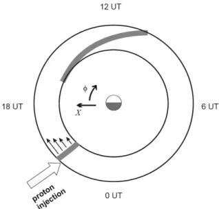
Fig. 2.The model of the source.
V=√g2ωdinstead of the angular velocity in Eq. (9). The
in-jection takes place at the instantt=0. For simplicity, we put the drift velocity to be proportional to the radial coordinate, ωd(x1)=dx1, whereddoes not depend onx1. As is easy
to see that in the course of time the cloud will be stretched into a spiral (Fig. 2).
In order to solve the wave Eq. (7), we perform the Fourier-transform of this equation overϕandt(see Appendix A). As a result, we obtain a differential equation only with respect to two variables,x1andx3:
ˆ
LA8mω= ˜qmω, (10)
whereωandmare the parameters of the Fourier transform over time (frequency) and azimuthal angle (azimuthal wave number), and
˜
qmω = −2mω√g
en0ωd
c2
× 1 2π
+∞
Z
−∞
2(t′)exp(iωt′−imωdt′) dt′.
In Eq. (10),LˆAis the Fourier-image of the Alfv´enic
opera-torLAanalogous to the Alfv´enic operator for the
monochro-matic wave with frequencyωand azimuthal wave numberm, defined as
ˆ LA≡
∂
∂x1LˆT(ω) ∂ ∂x1 −m
2Lˆ
P(ω),
where ˆ LT(ω)=
∂
∂x3 g2 √g∂x∂3 +
√g g1
ω2
A2
is the toroidal mode operator, and ˆ
LP(ω)=
∂ ∂x3
g1 √g∂x∂3 +
√g g2
ω2 A2,
is the poloidal mode operator. The eigenvalues of these oper-ators with the boundary condition on the ionosphere (8) are denoted T N andP N, respectively. They are called the
toroidal and poloidal eigenfrequencies since they character-ize the purely azimuthal (toroidal) and radial (poloidal) oscil-lations of field lines (e.g. Klimushkin et al., 2004; Leonovich and Mazur, 1997).
4 The structure of a single Fourier harmonic
The method of the solution of Eq. (10) has been developed by Klimushkin et al. (2004). As was shown there, the function 8mωcan be represented as
8mω≈RN(x1)TN(x1, x3), (11)
whereTN(x1, x3)is an eigenfunction of the toroidal operator
ˆ
LT, defining a longitudinal structure of theN-th harmonic
standing between ionospheres. The normalization condition is
*√ g
g1 TN2
A2 +
=1. (12)
(here the angle brackets designate integration along the field line between the ionospheres,h...i=Rx
3
+
x−3 (...)dx
3). The func-tionRN(x1)describes the structure of this harmonic across
the magnetic shells.
Let us introduce some definitions. The toroidal and poloidal eigenfrequencies are functions of the radial coor-dinatex1. If the wave frequencyωis fixed, we can introduce the notions of toroidalxT N1 and poloidalxP N1 magnetic shells determined as solutions of the equations
ω=T N(x1) (13)
and
ω=P N(x1), (14)
respectively. The distance between these shells is designated as 1N=xT N1 −xP N1 (in a cold plasma, 1N>0). In the
ma-jor part of the magnetosphere, the functionsP N(x1)and
T N(x1)are monotonically decreasing with the
characteris-tic scalel, which has the same order of magnitude as the size of the magnetosphere. For the sake of simplicity, we can then avail ourselves of the linear expansions
T N(x1)=0(1−
x1
l ) (15)
and
P N(x1)=0(1−
x1+1N
After substitution of expressions (13) and (14) into Eqs. (15) and (16), we obtain
xT N1 (ω)=l(1− ω 0
),
xP N1 (ω)=xT N1 −1N.
Further, if we substitute the function 8mω(x1, x3) from
Eq. (11) into Eq. (10), we obtain the ordinary differential equation defining the radial structure of the wave field:
∂ ∂x1(x
1
−xT N1 (ω)) ∂ ∂x1RN−
m2 L2(x
1
−xP N1 (ω))RN
=mq(x1, ω, m). (17) See Klimushkin et al. (2004), Leonovich and Mazur (1997) for more detail. Here
q(x1, ω, m)= q0 2π
+∞
Z
−∞
2(t′)exp(iωt′−imdx1t′) dt′,
q0= −el c2
ωd
0h
n0√gTNi. (18)
The solution of the Eq. (17) satisfying the boundary condi-tion (8) is
RN (x1, ω, m)
= iq0L
+∞
Z
−∞
dκ
+∞
Z
−∞
dt′ 2(κ+mt
′) 2(t′)
q
(κ2+m2l2 L2)(
L2 l22t′
2+1) × exp
iω(t′+m 0t
′+ κ
0)−imt
′+iκ(ξ−1)
+ imδN
l L(arctan
κL
ml +arctant
′L
l)
(19) (see Appendix B). The notations are:
ξ =x1/ l, δN=1N/ l, =dl.
5 The structure and evolution of the wave field
With the solution (10), we can solve the wave equation (7) by means of the reverse Fourier transform:
8(x1, x2, x3, t )=
+∞
Z
−∞
dω
+∞
Z
−∞
dm 8mωeimϕ−iωt. (20)
Thus, according to Eqs. (20, 11), the solution of the wave equation (7) is
8(x1, x2, x3, t )=RN(x1, x2, t ) TN(x1, x3), (21)
where the function
RN(x1, x2, t )=
+∞
Z
−∞
dω
+∞
Z
−∞
dm RN(m, ω) eimϕ−iωt (22)
defines both the transverse structure of the wave and its evo-lution. The expression forRN can be reduced to the form (see Appendix C):
RN(x1, x2, t )=iq0Lµ
×
+∞
Z
−∞
dm
+∞
Z
−∞
dκ 2(κ+mt )2(0t−κ) ei9(m,κ)
× "
(κ2+m 2l2
L2 )(
L2(0t−κ)2
l2 +(µ+m) 2)
#−1/2 (23)
where
9 (m, κ)=mϕ−m0t−κ
µ+m +κ (ξ−1) +mδN
l L
arctanκL
ml +arctan L
l
0t−κ µ+m
. (24) Since the drift angular velocityωdis assumed to be much less
than the Alfv´enic eigenfrequenciesT NandP N, the large
parameterµ=0/ appears. In this case the double inte-gral (23) can be evaluated by means of the stationary phase method (see Appendix D). Having done this calculation, we finally obtain the approximate expression forRN:
RN=A0ei90 (25) where the wave phase is
90≡9(κ0, m0)=m0(x1)ϕ−T N(x1)t
+ka(x1)1N
"
arctankr(x 1, ϕ, t )
ka(x1) +
arctanLϕ x1 #
, (26)
and the amplitude is
A0= i2π q0Lµ 2(ϕ)2(ωd(x
1)t−ϕ) [kr(x1, ϕ, t )2+ka(x1)2]1/2[x12+L2ϕ2]1/2
. (27) The factor2(ωdt−ϕ)in Eq. (27) shows that the wave field
is absent before the source in this approximation. Also, the following designations are introduced here: the radial com-ponent of the wave vector
kr(x1, ϕ, t )=
µ l t−
ϕ l2
x12 !
, (28)
the azimuthal component of the wave vector and the az-imuthal wave number
ka(x1)=
µ L
l−x1 x1 =
m0(x1) L , m0(x
1)
= T N(x 1)
ωd(x1)
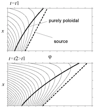
Fig. 3.The lines of the constant phase for different time instants.
6 Discussion
Let us discuss the main features of the solution obtained. The angular frequency of the wave is defined as
ω= ∂9
∂t =T N − 1N
l 0
1+kkr
a
−1
≈T N.
Hence, the frequency depends on the radial coordinate x1. Moreover, in the course of time ω is changed from P N
toT N. If we define the projection of the wave vector by
means of a similar procedure, that is as partial derivatives of the phase (26) askr=∂9/∂r,ka=∂9/∂ϕ, then their
ex-pression will differ from Eqs. (28, 29) only by small values, proportional to the parameterδN=1N/ l≪1. That means
that Eqs. (28, 29) can be safely used for needs of the qual-itative discussion. As is seen from those expressions, the azimuthal wave numbermalso depends on time, changing frommP=P N/ωd tomT=T N/ωd. But this dependence
is rather weak due to a small difference between toroidal and poloidal eigenfrequencies in cold plasma.
Much more important is a strong time dependence of the wave vector radial component. Near the line t−ϕ(l/x1)2=0, this value is very small,kr≪ka. As the
source is moving away from the points on this curve, the ra-dial component increases (Fig. 3). But according to Eqs. (6) and (25), the ratio betweenkrandkadefines the wave
polar-ization:|Ea/Er|=ka/ kr. Thus, just after the generation the
wave has a mixed polarization, and as the wave moves far-ther and farfar-ther away from the source, it becomes poloidally-polarized (Er≪Ea). Further, the wave finally transforms
Fig. 4.The wave electric field radial and azimuthal components at fixedx1andϕcoordinates.
into a toroidally-polarized one (Er≫Ea). The
characteris-tic transformation time is τ =2m0l
0L
. (30)
It is during this time span that the wave remained poloidally-polarized. An analogous transformation takes place also in the case of impulsive excitation (see, e.g. Klimushkin and Mager (2004)) with a similar transformation timeτ∼m/ω.
Such a double change of polarization was absent in the model where the drift velocity does not depend on the radial coordinate (Mager and Klimushkin, 2007). In the model con-sidered in the present paper the particle drift velocity grows with distance from the Earth. Consequently, the source stretches into strips at an acute angle to the surfacex1=const (as usual, the angle is measured counter-clockwise). Directly near the source the lines of the constant phase are parallel to the source (see Fig. 3). This means the presence of both ra-dial azimuthal components of the wave vector, that is, mixed wave polarization. Further evolution is accompanied by turn-ing of the lines of the constant phase counter-clockwise. At some time instant, there appears a point on a line of the con-stant phase where this line is tangent to thex2=const axis. At this point, the wave vector radial component equals zero, that is, the mode is poloidally polarized. Thus, the mode is poloidally polarized on the line passing through these points. Further, at a given point the constant phase line becomes in-clined at an obtuse angle to thex1=const surface, that is, the wave vector radial component appears again. In the course of time, the angle is increasing, i.e. the ratio|kr/ ka|is
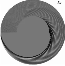
Fig. 5.The radial component of the electric field.
of electric field is shown, and also in Figs. 5–7, where the full wave structure is depicted. To compute these figures, wave attenuation due to finite ionospheric conductivity was taken into account.
With damping taken into account, Eq. (17) is written as ∂
∂x1(x 1
−xT N1 (ω)+ilγ 0
) ∂
∂x1RN− (31) −m
2
L2(x 1
−xP N1 (ω)+ilγ 0
)RN =mq(ω, m),
whereγ is a decrement of ionospheric damping. Having per-formed the manipulations described above, we obtain that in this case the expression (25) obtains one additional factor, namely
RN =A0e− γ ωd(ωdt−ϕ)
ei90. (32) Based upon this expression, we evaluate the width of the lo-calization region across magnetic shells. It is evident that the amplitude will be highest just near the source, i.e. in the vicinity of the curveωd(x1)t−ϕ=0. Thus, atγ t >1 the width
of the localization region will be 1L= L
γ t−1.
As is seen from this expression, the wave becomes more localized with time. For example, for the shell L=6, at γ=0.1ω andt=10T (where T is wave period), the width of the localization region is 1L≈1RE. As observations
show, high-mAlfv´en waves often have a localization width of∼1RE.
Let us evaluate the wave amplitude. On the basis of the Eqs. (18, 21, and 25), we obtain
8∼2π eL 2
c2µ hn0 √gT
NiTN∼
2π en0L2A2 c2µ .
Fig. 6.The azimuthal component of the electric field.
Fig. 7.The full electric field of the wave.
For this ordering, we used the normalization condition (12) for the eigenfunctionTN, which implies thatTN∼A/Land
hn0√gTNi∼n0AL. Further, from Eq. (6) we find the wave
electric and magnetic fields: E∼µ
L8∼
2π en0LA2
c2 , (33)
b∼ c AE∼
2π en0LA
c . (34)
Now, using Eq. (34), we can find which proton number den-sityn0in the drifting cloud is necessary for the generation of Alfv´en waves with observed magnetic field amplitudesb: n0∼
bc 2π eLA.
periods are of the order of 100 s, azimuthal wave numbers m∼20−100, they are frequently observed in the vicinity of L∼6 magnetic shell (Chisham et al., 1992). The characteris-tic value of the Alfv´en speed isA∼1000 km/s. To generate Alfv´en waves with such properties the number density must ben0∼10−2sm−3, which is much less than the background (cold) plasma density; the particle energyǫdetermining the velocity of proton drift in an inhomogeneous magnetic field (the source speed) must be about 50 keV (the azimuthal wave number of the generated wavem∼ω/ ). The particles with such energies are often observed simultaneously with high-moscillations.
7 Conclusions
Let us outline the general picture of the Alfv´en wave gen-eration by the moving plasma inhomogeneity. At a given point in the azimuthal coordinate, the wave appears just af-ter the source arrival. Under the realistic assumptions of the particle energy and density in the moving source, the ampli-tudes of the generated oscillations are close to those really observed. The direction of the wave propagation coincides with the direction of the source movement, the wave polar-ization is intermediate between poloidal and toroidal. As the source moves off the given point, the wave transforms first into a poloidal and then into toroidal wave. Note the oscil-latory structure of the wave field behind the source, which is a consequence of the finite size of the cloud along the field line (as we assumed the source to be distributed between the conjugated points of the ionosphere). Earlier, Zolotukhina (1974) and Neubauer (1980) showed that the Alfv´en wave excited by a compact moving cloud (that is, by a source much shorter than the field line) constituted current (Alfv´en) wings, spreading from the source. Since a finite source can be repre-sented as a superposition of many compact sources, the oscil-latory structure obtained in this paper can be viewed as a re-sult of the interference of such wings. Just after the injection of the cloud, when the cloud is continuing to spread along the field line (within few first bounce periods), the wave field probably resembles pure Alfv´en wings. However, the evo-lution just after the injection has not been considered in this paper.
The mechanism considered in the paper provides a way for explaining the features of the observed azimuthally small scale waves mentioned in the Introduction:
1. The azimuthal wave numbermis fully determined by the eigenfrequency of the wave standing between iono-spheres, ω∼T N(x1), and the drift velocity of the
source, ωd: m∼ω/ωd. This explains why observed
waves have well-definedmvalues.
2. In accordance with the observations, the phase velocity of the poloidal Alfv´en waves coincides with the direc-tion of the proton drift.
3. Despite its transformation from poloidal to toroidal, at a given point in azimuth the wave remains poloidal dur-ing a rather large time spanτ∼m/ω∼ω−d1, which cor-responds to a sufficiently large angular distance from the sourceφ=τ∼1. Besides, in some sense the wave is always poloidal, because the source continues its az-imuthal movement, generating the poloidal wave at new points.
4. If the wave attenuation is taken into account (for ex-ample, due to finite conductivity of the ionosphere or wave-particle interaction), then the wave does not have enough time to transform into toroidal, and the maxi-mum wave amplitude will correspond to a mixed polar-ization, depending on the observation point.
5. Besides, the wave damping leads to a localization across the magnetic shells, which corresponds to observational data for the high-mwaves. If the azimuthal coordinate is fixed, in the course of time the localization region will shift toward the Earth.
As was mentioned in the Introduction, some of these fea-tures of the high-mwaves cannot be explained by the theory of drift-bounce instability. It must be noted, however, that the wave-particle energy exchange can lead to a further am-plification or attenuation of the wave. Besides, a ponderomo-tive force can appear, which governs feedback of the gener-ated field upon the generating particles, which can result in the formation of the stationary ring current. However, these questions are far beyond the topic of the present paper.
Appendix A
The derivation of Eq. (7)
Fourier-transformation of Eq. (7): 1
(2π )2
+∞ Z −∞ dϕ +∞ Z −∞
d t eiωt−imϕLA8=
= − 1 (2π )2
+∞ Z −∞ dϕ +∞ Z −∞
d t eiωt−imϕ4π c2
√g ∂ ∂x2
∂ ∂tj
2 ext.
We replacex2byϕinLAand the right side of this equation. Sinceg1,2andgare independent ofϕandt then for the left side of this equation we have
− ∂x∂1 √g g1 1 A2 ∂ ∂x1 1 (2π )2
+∞ Z −∞ dϕ +∞ Z −∞
d t eiωt−imϕ ∂ 2
∂t28
+ ∂ ∂x1
∂
∂x3 g2 √g∂x∂3
∂
∂x1 1 (2π )2
+∞ Z −∞ dϕ +∞ Z −∞
d t eiωt−imϕ8
− √g g2 1 A2 1 (2π )2
+∞ Z −∞ dϕ +∞ Z −∞
d t eiωt−imϕ ∂ 2
∂t2 ∂2 ∂ϕ28
+ ∂x∂3√g1g∂x∂3 1 (2π )2
+∞ Z −∞ dϕ +∞ Z −∞
d t eiωt−imϕ ∂ 2
∂ϕ28.
After integrating by parts we obtain: ∂ ∂x1 √g g1 ω2 A2 ∂ ∂x1 1 (2π )2
+∞ Z −∞ dϕ +∞ Z −∞
d t eiωt−imϕ8
+ ∂x∂1 ∂ ∂x3
g2 √g∂x∂3
∂ ∂x1
1 (2π )2
+∞ Z −∞ dϕ +∞ Z −∞
d t eiωt−imϕ8
−m2 √g
g2 ω2
A2 1 (2π )2
+∞ Z −∞ dϕ +∞ Z −∞
d t eiωt−imϕ8
−m2 ∂ ∂x3
g1 √g∂x∂3
1 (2π )2
+∞ Z −∞ dϕ +∞ Z −∞
d t eiωt−imϕ8.
Here 1/(2π )2
+∞R
−∞
dϕ
+∞R
−∞
d t eiωt−imϕ8≡8mω.
For the right side, after substitutingjext2 in the explicit form (9) we have
− 4πc2
√ge n0ω
d
1 (2π )2
+∞ Z −∞ dϕ +∞ Z −∞
d t eiωt−imϕ
× ∂ ∂ϕ
∂
∂tδ(ϕ−ωdt ) 2(t )
= −mω4π c2
√ge n 0ωd
1 (2π )2
+∞
Z
−∞
d t 2(t )eiωt−imωdt ≡ ˜q mω.
Appendix B
The derivation of Eq. (19)
We solve Eq. (17) by means of the Fourier transform. Let us put
RN(x1)=
+∞
Z
−∞
eikx1RN(k) dk, (B1)
then
RN(k)=im k
Z
−∞
dk′ iq(k
′)
q
(k′2+k2
y)(k′2+ky2)
×exp[i(k−k′)xT N1 +iky1N(arctan
k ky −
arctank
′
ky
)],
whereky=m/L,
q(k′)= 1 2π
+∞
Z
−∞
e−ikx1q(x1) dx1=
= q0 (2π )2
+∞
Z
−∞
dt′eiωt′2(t′)
+∞
Z
−∞
dx1e−ik′x1−imdxt′ =
= q0 2π
+∞
Z
−∞
dt′eiωt′2(t′)δ(k′+mdt′).
Then we integrate overk′, substitute the expression obtained into Eq. (B1) and introduce new variablesx1=lξ,k=κ/ l. As a result we obtain Eq. (19).
Appendix C
The derivation of Eq. (23)
After substitution of Eq. (19) into Eq. (22) we obtain the ex-pression forRNas the integral
RN=iq0L
× 2(κ+mt
′) 2(t′)
q
(κ2+m2l2 L2)(
L2 l22t′
2+1) ×exp
iω(t′+m 0t
′+ κ
0)−imt
′+iκ(ξ−1)
+imδN
l L(arctan
κL
ml +arctant
′L
l)
. (C1) First we integrate overω, which gives us δ(t′+m
0t
′+ κ 0) in the subintegral function, then we integrate the expression obtained overt′. As a result, Eq. (C1) reduces to the simpler form (23) with only two integrations.
Appendix D
The stationary phase method
Let us introduce the large parametersµ=0/ ≫1 (Since the drift angular velocity is assumed to be much less than the toroidal and poloidal eigenfrequencies), and small parame-terδN=1N/ l≪1 (since the distance between toroidal and
poloidal surfaces1N is much less that the scale of the
mag-netosphere). Let us find the point of the stationary phase (m0, κ0)through the conditions
∂9 ∂κ
m0,κ0
=0, ∂9
∂m
m0,κ0 =0.
After we neglect the terms proportional to the small param-eterδN, we obtain two equations, which determine the
posi-tion of this point: ξ−1+mm0
0+µ =
0, (D1)
ϕ−µ 0t−κ0
(m0+µ)2 =0. (D2) We find from these equations that
m0=µ 1−ξ
ξ ,
κ0=µ(t−ϕξ−2).
Thus, we find the wave phase: Eq. (26). Further, following the stationary phase method, we find the expression deter-mining the wave amplitude:
A0=Ae0
+∞
Z
−∞
dκ
+∞
Z
−∞
dm exp[i1
2A(κ−κ0) 2
+i1
2B(m−m0) 2
+iC(κ−κ0)(m−m0)], where
e
A0= r iq0Lµ2(κ0+m0t )2(0t−κ0)
L2
l2(0t−κ0)2+(µ+m0)2 κ0+m0l 2 L2
,
A= ∂ 29
∂κ2
m0,κ0 ∼ δµN,
B= ∂ 29
∂m2
m0,κ0 ≈2ξ
µ,
C= ∂ 29
∂κ∂m
m0,κ0 ≈ ξ
2
µϕ.
It is seen thatA≪C, B. Thus, we have
A0=Ae0
+∞
Z
−∞
dm eiξµ(m−m0)2
+∞
Z
−∞
dκ eiξ 2
µϕ(κ−κ0)(m−m0) =
=Ae0
+∞
Z
−∞
dmei ξ
µ(m−m0)22π µ
ξ2δ(m−m0)=Ae02π µ ξ2.
As a result, after some algebra, we obtain the expression (27) for the wave amplitude.
Acknowledgements. The work is supported by INTAS grant 05-1000008-7978, RFBR grant 07-05-00185, Program of presidium of Russian Academy of Sciences #16, and OFN RAS #16. The work of P. N. Mager was also supported by Russian Science Support Foun-dation.
Topical Editor I. A. Daglis thanks S. Buchert and L. Ozeke for their help in evaluating this paper.
References
Akhiezer, A. I., Akhiezer, I. A., Polovin, R. V., Sitenko, A. G., and Stepanov, K. N.: Collective oscillations in a plasma, M.I.T. Press, Cambridge, Massachusetts, 1967.
Akhiezer, A. I., Akhiezer, I. A., Polovin, R. V., Sitenko, A. G., and Stepanov, K. N.: Plasma electrodynamics. Vol. 1: Linear theory (International Series of Monographs in Natural Philosophy, Vol. 68), Oxford, Pergamon Press, 1975.
Allan, W., Poulter, E. M., and Nielsen, E.: STARE observations of a Pc5 pulsations with large azimuthal wave number, J. Geophys. Res., 87, 6163–6172, 1982.
Allan, W., Poulter, E. M., and Nielsen, E.: Pc5 pulsations associated with ring current proton drift: STARE radar observations, Planet. Space Sci., 31, 1279–1289, 1983.
Anderson, B. J.: Statistical studies of Pc3–5 pulsations and their relevance for possible source mechanisms of ULF waves, Ann. Geophys., 11, 128–143, 1993,
http://www.ann-geophys.net/11/128/1993/.
Baddeley, L. J., Yeoman, T. K., Wright, D. M., Davies, J. A., Trat-tner, K. J., and Roeder, J. L.: Morning sector drift-bounce res-onance driven ULF waves observed in artificially-induced HF radar backscatter, Ann. Geophys., 20, 1487–1498, 2002, http://www.ann-geophys.net/20/1487/2002/.
Baddeley, L. J., Yeoman, T. K., Wright, D. M., Trattner, K. J., and Kellet, B. J.: On the coupling between unstable magnetospheric particle populations and resonant highmULF wave signatures in the ionosphere, Ann. Geophys., 23, 567–577, 2005a, http://www.ann-geophys.net/23/567/2005/.
Baddeley, L. J., Yeoman, T. K., and Wright, D. M.: HF doppler sounder measurements of the ionospheric signatures of small scale ULF waves, Ann. Geophys., 23, 1807–1820, 2005b, http://www.ann-geophys.net/23/1807/2005/.
Chisham, G., Orr, D., and Yeoman, T. K.: Observations of a giant pulsation across an extended array of ground magnetometers and on auroral radar, Planet. Space Sci., 40, 953–964, 1992. Fenrich, F. R., Samson, J. C., Sofko, G., and Greenwald, R. A.: ULF
high- and low-mfield line resonances observed with the Super Dual Auroral Radar Network, J. Geophys. Res., 100, 21 535– 21 548, 1995.
Eriksson, P. T. I., Blomberg, L. G., Walker, A. D. M., Glassmeier, K.-H.: Poloidal ULF oscillations in the dayside magnetosphere: a Cluster study, Ann. Geophys., 23, 2679–2686, 2005,
http://www.ann-geophys.net/23/2679/2005/.
Eriksson, P. T. I., Blomberg, L. G., and Glassmeier, K.-H.: Cluster satellite observations of mHz pulsations in the dayside magneto-sphere, Adv. Space Res., 38, 1730–1737, 2006.
Glassmeier, K.-H.: Magnetometer array observations of a giant pul-sation in the magnetosphere, J. Geophys., 48, 138–147, 1980. Glassmeier, K.-H.: ULF pulsations, Handbook of Atmospheric
Electrodinamics, II, 463–502, 1995.
Glassmeier, K.-H., Buchert, S., Motschmann, U., Korth, A., and Pedersen, A.: Concerning the generation of geomagnetic giant pulsations by drift-bounce resonance ring current instabilities, Ann. Geophys., 17, 338–350, 1999,
http://www.ann-geophys.net/17/338/1999/.
Guglielmi, A. V. and Zolotukhina, N. A.: Excitation of Alfv´en os-cillations of the magnetosphere by the asymmetric ring current, Issled. geomagn. aeron. i fiz. Solntsa, 50, 129–137, 1980 (in Rus-sian).
Gurnett, D. A.: On a remarkable similarity between the propagation of whistlers and the bow wave of a ship, Geophys. Res. Lett., 22, 1865–1868, 1995.
Hughes, W. J., Southwood, D. J., Mauk, B., McPherron, R. L., and Barfield, J. N.: Alfv´en waves generated by an inverted plasma energy distribution, Nature, 275, 43–44, 1978.
Karpman, V. I., Meerson, B. I., Mikhailovsky, A. B., and Pokhotelov, O. A.: The effects of bounce resonances on wave growth rates in the magnetosphere, Planet. Space. Sci., 25, 573– 585, 1977.
Klimushkin, D. Yu.: The propagation of high-mAlfv´en waves in the Earth’s magnetosphere and their interaction with high-energy particles, J. Geophys. Res., 105, 23 303–23 310, 2000.
Klimushkin, D. Yu.: How energetic particles construct and destroy poloidal high-mAlfv´en waves in the magnetosphere, Planet. Space Sci., 55, 722–730, 2007.
Klimushkin, D. Yu. and Mager, P. N.: The spatio-temporal structure of impulse-generated azimuthal small-scale Alfv´en waves inter-acting with high-energy charged particles in the magnetosphere, Ann. Geophys., 22, 1053–1060, 2004,
http://www.ann-geophys.net/22/1053/2004/.
Klimushkin, D. Yu., Mager, P. N., and Glassmeier, K.-H.: Toroidal and poloidal Alfv´en waves with arbitrary azimuthal wave num-bers in a finite pressure plasma in the Earths magnetosphere, Ann. Geophys., 22, 267–288, 2004,
http://www.ann-geophys.net/22/267/2004/.
Leonovich, A. S. and Mazur, V. A.: A model equation for monochromatic standing Alfv´en waves in the axially-symmetric magnetosphere, J. Geophys. Res., 102, 11 443–11 456, 1997. Mager, P. N. and Klimushkin, D. Yu.: Spatial localization and
azimuthal wave numbers of Alfv´en waves generated by drift-bounce resonance in the magnetosphere, Ann. Geophys., 23, 3775–3784, 2005,
http://www.ann-geophys.net/23/3775/2005/.
Mager, P. N. and Klimushkin, D. Yu.: Generation of Alfv´en waves by a plasma inhomogeneity moving in the Earths Magneto-sphere, Plasma Physics Reports, 33, 391–398, 2007.
Neubauer, F.: Nonlinear standing Alfv´en wave current system at Io – Theory, J. Geophys. Res., 85, 1171–1178, 1980.
Pilipenko, V., Kleimenova, N., Kozyreva, O., Engebretson, M., and Rasmussen, O.: Long-period magnetic activity during the May 15, 1997 storm, J. Atmos. Sol.-Terr. Phys., 63, 489–501, 2001. Sch¨afer, S, Glassmeier, K.-H., Eriksson, P. T. I., Pierrard, V.,
For-nasson, K.-H., and Blomberg, L. G.: Spatial and temporal char-acteristics of poloidal waves in the terrestrial plasmasphere: A CLUSTER Case Study, Ann. Geophys., 25, 1011–1024, 2007, http://www.ann-geophys.net/25/1011/2007/.
Southwood, D. J.: Low frequency pulsation generation by energetic particles, J. Geomagn. Geoelectr., Suppl. II, 32, 75–88, 1980. Wright, D. M., Yeoman, T. K., Rae, I. J., Storey, J., Stockton-Chalk,
A. B., Roeder, J. L., and Trattner, K. J.: Ground-based and Polar spacecraft observations of a giant (Pg) pulsation and its associ-ated source mechanism, J. Geophys. Res., 106, 10 837–10 852, 2001.