Working
Paper
348
Exchange rate misalignments,
interdependence, crises, and currency
wars: an empirical assessment
Emerson Fernandes Marçal
CEMAP - Nº 03
Working Paper Series
WORKING PAPER 348–CEMAP Nº 03•DEZEMBRO DE 2013• 1
Os artigos dos Textos para Discussão da Escola de Economia de São Paulo da Fundação Getulio
Vargas são de inteira responsabilidade dos autores e não refletem necessariamente a opinião da
FGV-EESP. É permitida a reprodução total ou parcial dos artigos, desde que creditada a fonte.
Exchange rate misalignments, interdependence, crises, and currency wars: an empirical assessment1
Emerson Fernandes Marçal
CEMAP-EESP-FGV and CCSA-Mackenzie. E-mail: [email protected]
(October 2013)
ABSTRACT
This study aims to compare two different methodologies of calculating exchange rate misalignment and test whether there is interdependence among countries in determining the real effective exchange rate. Two different econometric approaches are used to achieve these goals. The first one involves estimating a multivariate time series model that contains only
country-specific variables and evaluating if this basic model can be improved by adding other countries’
variables. The study uses the algorithm suggested by Hendry et al. to select the best model specification. The second strategy involves estimating long panel data with the real effective exchange rate and fundamentals for a group of countries and explicitly testing the interdependence hypothesis. The results suggest that the long-run exchange rate is mainly driven by its own fundamentals for most countries. The existence of interdependence is restricted to short-run dynamics.
Keywords: Real effective exchange rate, cointegration, exchange rate misalignment JEL codes: E00, F31, C30
RESUMO
Este trabalho tem por objetivo comparar metodologias distintas para cálculo de desalinhamento cambial além de testar a hipótese se as taxas de câmbio dos diversos países sofrem influencia apenas dos seus próprios fundamentos ou também da taxa de câmbio e dos fundamentos de outros países. Estas hipóteses consistem, respectivamente, na ausência ou na existência de interdependência entre os diversos países. Para realizar tal tarefa utilizam-se duas estratégias empíricas. A primeira baseia-se em avaliar se um modelo multivariado de séries de tempo usualmente utilizada na literatura de desalinhamento cambial com dados apenas do próprio país em análise pode ser melhorado através da adição de variáveis relacionadas a outros países usando o algoritmo proposto por David Hendry e co-autores. A segunda estratégia consiste em estimar um panel longo com as variáveis utilizadas para estimar desalinhamento cambial e testar formalmente a hipótese de ausência de interdependências. Os resultados sugerem que em ambas estratégias existe evidência de existência de interdependência. Esta ocorreria mais por conta de fatores ligados ao curto prazo, ou seja, o que explicaria o valor da taxa de câmbio de um país no longo prazo seriam seus próprios fundamentos enquanto no curto prazo fatores externos poderiam causar desvios.
1
1.
Introduction
The exchange rate is an important macroeconomic variable and its variation affects global and sectorial economic activity, prices and interest rates, and trade flows. Large fluctuations of the exchange rate exacerbate debates regarding whether such movements are “excessive,” reflect “fundamentals,” or are “rational.”
Empirical literature on the exchange rate has advanced toward building models for assessing the long-term determinants of real exchange rates. Empirical strategies can be formulated based on models that use the doctrine of Purchasing Power Parity or an analysis based on fundamentals.2
Given this second approach, in this study, I estimate the long-term determinants of the real exchange rate of the G-20 as well as certain other selected countries. From these models, I construct the estimates of exchange rate misalignment for each country and test whether there is interdependence between various currency misalignments. The remainder of this paper is organized in the following manner. In the second section, I discuss the importance of exchange misalignment. In the third section, I conduct a non-exhaustive review of existing literature. In the fourth section, I discuss the econometric methodology employed in greater detail. In the fifth section, I present the results and compare them with those of similar studies in existing literature. In the last section, I present some conclusions.
2
2.
Motivation
The severity of the crisis in the US economy in 2008 brought the fear of a strong negative contagion in the rest of the world. Among other measures, the US authorities adopted an aggressive monetary policy with a strong reduction in nominal interest rates and monetary expansion. According to analysts, such measures generated strong pressure for US dollar depreciation against currencies of countries whose governments did not follow a similar monetary policy of lowering their domestic interest rates. If a country chooses not to follow such a reduction and opts to keep interest rates unchanged and accumulate reserves to prevent appreciation of its currency, it will eventually have to face inflation pressures. Some authors argue that the Federal Bank, after the sub-prime crisis, has been trying to use monetary policy to generate a depreciation of the dollar rate to create an aggregate demand stimulus to speed up economic recovery. This policy has generated worldwide repercussions, and the possible disadvantages of such effects are a subject of debate.
One of the channels through which the monetary policy functions is real exchange rate depreciation. If the effect on other countries is deleterious, these countries could attempt to use available instruments to avoid the appreciation of their local currencies. This might configure a policy known in the literature as “beggar thy neighbor.”3 Countries can adopt measures to prevent the appreciation of their currencies to avoid internalizing the costs of a deliberate expansionary monetary policy (“quantitative easing”).4
A cost-benefit analysis of this policy should be conducted not only for ascertaining its short-term effects but also for its long-term effect on output, inflation,
3
Eichengreen, B. and J. D. Sachs (1986). Exchange rates and economic recovery in the 1930s, National Bureau of Economic Research Cambridge, Mass., USA.
4
and the welfare of countries. The countries’ strategic choice should aim to obtain short-term economic gains through an expansionary monetary policy despite being exposed to suffering some sort of retaliation from partners. It is also important to analyze the circumstances under which a country’s partners do not retaliate and accept the costs of appreciation as the best strategy.
For a small country, the strategy of attempting to retaliate is perhaps not the best as it is very difficult to cause significant damage to a leader country, thereby rendering such a policy ineffective. The main mechanism by which monetary policy would function is via devaluation of the exchange rate; however, for a small country, it would be difficult to counteract the effects of exchange rate appreciation by changing its own monetary policy. Turnovsky et al. (1987) is an example of a study in which this strategic interaction is formally analyzed.
3.
Literature on exchange rate misalignment
The existing literature on the real exchange rate is vast. The classical doctrine and perhaps one of the oldest one is Purchasing Power Parity (PPP). Reference to this theory can be found in classical economics. Recently, some studies have collected evidence in favor of the validity of PPP for tradable goods, although the adjustment toward equilibrium can be very slow (Froot and Rogoff (1995)). Ahmad and Craighead (2010) analyzed monthly consumer price indexes for a secular American and British data set. The study showed strong evidence in favor of mean reversion, but with a high half-life. Their work follows Taylor’s guidelines (Taylor (2001)).
3.1.The economics of exchange rate misalignment
There is a theoretical discussion on the variables that drive the exchange rate in the long run. Two old but very important references are Edwards (1987) and Dornbusch (1976). The first analyzes economic misalignment, its causes, and consequences. The second is the classical model of flexible exchange rates. They analyze how monetary policy shocks can cause deviations from long-term PPP and the phenomena of under and over shooting.
Stein (1995) proposes the natural rate of exchange approach (NATREX). According to the study, the equilibrium exchange rate level is determined at the point at which investment and savings generated by economic fundamentals are equal.
A classical reference to exchange rate misalignment is made by Williamson (1994). He defines equilibrium exchange rate as the level at which the country is able to maintain a certain desired level of deficit or surplus (seen as sustainable) in its external accounts. This is called the fundamental approach of the real exchange rate (FRER). Cline (2008) is another reference in this regard.
One source of criticism comes from the fact that there is a high degree of arbitrariness in choosing the desirable level of external accounts. Another source of criticism comes from the focus of the approach on flows and not on stocks.
Faruqee (1995) seeks to incorporate issues related to the evolution of stocks and builds a model in which there is an interaction between flows and stocks. Therefore, he shows that there must be a stable relationship between real exchange and the net foreign investment position between residents and non-residents. This is called the behavioral approach of the real exchange rate (BRER). The model was extended by Alberola et al. (1999). Further, Kubota (2009) developed a model with intertemporal consumption choice and capital accumulation. The model suggests that the real exchange rate is a function of relative terms of trade, net external position, and relative productivity of tradable and non-tradable sectors. This is the approach used in the current study.
4.
Econometric methodology
In this study, we propose to test whether the models estimated using a traditional approach to calculate currency misalignment from a list of fundamentals can be improved upon by modeling with long panel data that take into account a possible interdependence among different countries. In order to this, two testing strategies are used.
4.1.Testing Strategies
4.1.1.Strategy 1
The starting point is Larsson and Lyhagen’s model (Larsson and Lyhagen (2007)). It is a generalization of Johansen and Juselius’ procedure (Johansen (1988), Johansen (1995), and Juselius (2009)).
Let xit [CRERit Fundamentoit] be the vector that contains the real exchange
rate and its fundamentals at time t for country i, and let Xt [x'1t ... x'Nt]' be the vector in which country data are stacked.
The general model is given by the following equation: (1) Xt 1Xt kXtk DtAB'Xt1t
1 ...
where t represents random errors, and is its variance and covariance matrix
of the shocks. Shocks are assumed to be uncorrelated in time and cross-sectional dimensions. The vector Xt contains the data series from all countries, Dt contains
deterministic terms, and {1,...,k,,A,B} denotes the set of parameters to be
estimated. In the general case, all the variables could cointegrate with each other5, but
5
Larsson and Lyhagen (2007), for example, restrict their analysis to the case in which there can be cointegration only between variables of the same country. Then,
(2)
N B
0
0
1
,
where i is a vector of dimension pxr.
The matrix of load (A) has no a priori constraint and enables all sorts of configuration, provided that the system is stable. One cointegrated vector that contains the variables of one country can generate not only part of the equation of that country but also other countries’ equations. It is precisely this possibility that makes this structure attractive for analyzing the problem considered in this work.
For example, it is possible to test if the cointegration vector, which represents the fundamentals of a country (e.g., US), is present in exchange rates and fundamentals variables’ equations. This hypothesis could be tested under the null hypothesis that certain elements of matrix A are zero. Larsson and Lyhagen (2007) showed that after the rank of a long-run matrix is determined, the test can be implemented using a likelihood ratio test with an asymptotic chi-squared distribution. The authors also derived a test to determine the rank of cointegration; this test has no standard asymptotic distribution, and this distribution was tabulated. Among other interesting hypotheses, it is also possible to test jointly, for example, whether the net external investment position is one of the fundamentals for all analyzed countries.
dimensions. We decided to estimate models for all combinations of countries taken as pairs for a sample with data from 1981 to 2011, and a model of higher dimension with five developed countries and Brazil using a larger sample (beginning in 1970).
4.1.2.The estimation
The estimation of the model is done by using the algorithm of generalized reduced rank regression (GRRR) developed by Hansen (2003). All restrictions imposed on the general model can be tested using a likelihood ratio test with an asymptotic chi-squared distribution.
In the following subsection, we present the algorithm of the generalized reduced rank regression
4.1.2.1.
Estimating a panel VECM using generalized reduced rankregression
Defining the following variables and arrays:
(3)
t t t
2t 1 t 1t
t ot
D
ΔX ΔX
Z X Z
ΔX
Z
k
...
and
(4) C(Γ1,...,Γk1,Φ)
yields
(5) Z0t AB'Z1tCZ2tεt
Hansen (2003) shows how to estimate the process given in (5). Some definitions are now necessary:
where H is known, φ contains free parameters, h is a tool for normalization, and vec is an operator that transforms a matrix in a column vector. 6
(7)vec(A,C)Gψ,
where G is known, and ψ contains free parameters.
Using (6), (7), and (8) to (11), it is possible to estimate the model parameters (see Hansen (2003) for details):
(8)
T 1 t ' 2t ' 1t ot 1 1 T 1 t 1 ' 2t 2t ' 1t 2t ' 2t 1t ' 1t 1t )) Z , B (Z Z (t) Ω vec( xG' x G (t) Ω Z Z B Z Z Z Z ' B B Z Z ' B G' G C , A ˆ ˆ ˆ ˆ ˆ ˆ ˆ ) ˆ ˆ ( vec , (9) h )h Z Z A (t) Ω ' A vec( ) A (t) Ω )' Z C (Z vec(Z H' xH' x )H Z Z A (t) Ω ' A ( H' H B T 1 t ' 1t 1 T 1 t 1 2t 0t 1t 1 T 1 t ' 1t 1t 11 t
ˆ ˆ ˆ ˆ ˆ ˆ ˆ ˆ ˆ ) ˆ ( vec , (10)
T t T 11 ˆ ˆ
) ( ˆ
t tε'
ε
Ω , and
(11) εˆt Z0tAˆBˆ'Z1tCˆZ2t.
After convergence is attained according to some established criterion, the likelihood function can be calculated. Based on the values of the restricted and unrestricted general model, it is possible to calculate a likelihood ratio test with an asymptotic chi-squared distribution (Larsson and Lyhagen (2007)).
4.1.2.1.
Testing linear restrictions on panel VECM parametersThe likelihood ratio procedure described in the previous section suffers from a serious distortion. This encourages analysts to use a bootstrap technique to obtain
6
appropriate critical values. Studies that discuss similar problems are Johansen (1999), Johansen (2000), Gredenhoff and Jacobson (2001), and Swensen (2006). We chose to perform a bootstrap to simulate the appropriate distribution for the test statistic. The results suggest that the size distortion is actually severe.
The procedure used is a wild bootstrap similar to that used in Cavaliere et al. (2008):7
Step 1: Estimate the model given by equation (3) under the null and alternative hypothesis and calculate the statistic likelihood ratio.
Step 2: Save the model parameters estimated under the null hypothesis and check the stability of the system. If the system is stable, proceed to Step 3. If not, abort the procedure.
Step 3: Construct the errors for generating artificial data using equation (12) below from the parameters estimated with the model constraints on the null hypothesis:
(12) u~t εˆtwt,
where εˆt is defined as in (11) and wt ~ NI(0,1).
Step 4: Generate the Q series with the sample size T from equation (1) with the parameter structure of the null hypothesis.
Step 5: Perform the likelihood ratio test described in Step 1 for all artificially generated samples. The values of the test statistics are retained. Calculate the p-value by dividing the total number of times the value of the likelihood ratio statistic obtained with the real sample data is greater than value of the likelihood ratio statistic obtained with artificial data divided by the number of runs.
7
4.1.3.Strategy 2
The second strategy for testing the existence of interdependence involves estimating multivariate models. First, a country-by-country analysis is done to obtain the long-term relationships that will be used as input for the construction of the exchange rate misalignment estimate. Then, the error correction mechanisms obtained for all countries are included in each individual country model. Thereafter, their relevance is tested using the algorithm suggested by Santos et al. (2008) and Hendry and Krolzig (2005). This procedure was implemented using software Oxmetrics. If the final selected model contains only the series of the individual country, it can be concluded that there is no evidence for the interdependence hypothesis, whereas in the event that the final country model contains variables related to other countries, it can be concluded that there is some degree of interdependence.
4.2. Gonzalo and Granger’s decomposition
Many decomposition methods have been suggested for the decomposition of the process between permanent and transitory components. In general, the decomposition has the following form:8
(13) Xt (c')1c'Xt c('c)1'Xt.
The decompositions vary according the choice of vector c. A condition for the existence of the decomposition is that the matrix ('c) has full rank. However, this condition is not always satisfied.
Gonzalo and Granger (1995) propose that c.9 This representation always exists for the case of a VECM of zero order. Johansen (1995) proposes that c.
8
This decomposition exists in the system since there are variables whose order of integration is at most 1.10 Kasa (1992) proposes that c. Another possibility is to generate forecasts from the VECM estimated for each point. The values for which the series converge are the fundamentals. In this study, I use the decomposition given by Gonzalo and Granger (1995).11
In Gonzalo and Granger’s decomposition, there is no Granger causality between transitory and permanent components in that the former do not12 cause a change in permanent components in the long run; in other words, the exchange rate misalignment, defined as the transitory component of the real exchange rate equation in a multivariate system, does not contain information that is relevant for predicting the change in the permanent components in the long run.13 Gonzalo and Granger’s decomposition is widely used in the literature of exchange rate misalignment. See, for example, Alberola et al. (1999).
5.
Database description
The data for this study were collected from the International Financial Statistics of the International Monetary Fund (IMF). The real exchange rate for each country is
9 Go zalo a d Gra ger’s deco positio —Gonzalo, J. and C. W. J. Granger (1995). "Estimation of
Common Long-Memory Components in Cointegrated Systems." Journal of business and Economics Statistics 13(1)—was implemented in Matlab software.
10
Note that in (13), the condition for matrix C()1' to exist is that the inverse of matrix can be calculated. This is a direct implication of the representation theorem of Granger—Johansen (Johansen, S. (1995). Likelihood-based inference in cointegrated vector autoregressive models. Oxford, Oxford University Press.).
11
In this case, the components of the deterministic model as constant and time trends should be restricted to the space of cointegration.
12
For a rigorous definition of Granger causality, see Hendry (Hendry, D. F. (1995). Dynamic Econometrics. Oxford, Oxford University Press.).
13
If the most appropriate VECM contains only the erroneous mechanism and deterministic terms, then Gonzalo and Granger’s deco positio (Gonzalo, J. and C. W. J. Granger (1995). "Estimation of Common Long-Memory Components in Cointegrated Systems." Journal of Business and Economics Statistics
calculated from a basket of currencies that uses data from consumer price indexes. The data on net foreign investment position and reserves have been collected by the IMF from 2000 onward and those for previous years were collected on the basis of those given in Lane and Milesi-Ferretti (2007). The gross domestic product data were collected from the World Bank World Development Indicators available online.
The codes were run in Matlab and Oxmetrics software, and the frequency is annual. In many cases, data begins in 1970 and ends in 2010; in other cases, the sample begins in 1980 and ends in 2010. The countries that are analyzed are Australia, Brazil, Canada, Colombia, Denmark, Finland, France, Germany, Greece, India, Italy, Portugal, Ireland, Japan, Mexico, Netherlands, South Korea, South Africa, Singapore, Spain, Sweden, United Kingdom, Uruguay, Turkey, and the United States. Data from 1970 until 2012 is not available for all countries. However, all listed countries at least have information from 1980 onward.
6.
Results
As a first step, analysis tests were conducted using multivariate cointegration (Johansen (1988)). For countries that showed significant relationships, the error correction mechanisms were calculated. Table 20 contains the results of cointegration tests (Johansen (1988), Shin (1994), and Engle and Granger (1987)). The estimated error correction mechanism was used as input for strategy 2. Moreover, the error correction mechanisms were again estimated for strategy 1.
6.1.1.Long panel data (1970–2010): Australia, Brazil, Canada,
the United States, Japan, and the United Kingdom
In order to investigate the existence of interdependence among exchange rate misalignments in the above countries, I estimated the model of equation (1). The model under the null hypothesis is given by
(14) N B 0 0 1 and N A 0 0 1 .
Except for the variance and covariance matrices of the shocks, there is no source of interdependence. In the alternative hypothesis, matrices A and B are completely unrestricted.
The results of this test are presented in Table 1. Based on the asymptotic value, the null hypothesis is easily rejected, but it is accepted if bootstrap critical values are used. Since the tests can suffer from size distortions, I tend to rely on the option of not rejecting the null.
Likelihood Ratio Test:
Test Statistic 689,67 Number of restrictions 180 asymptotical p-value 0,00% bootstrap p-value* 28,10% * 300 replications.
Table 1: Results of the test for assessing the existence of interdependence based on misalignments in
6.1.2.Peer analysis: Using data from 1980–2011 and N = 2
The second group of estimates was conducted using pairs of countries. The results are presented in Table 2. Again, the difference between the asymptotic critical and simulated critical values is large. As a general rule, the simulated critical values were consistently larger than the asymptotic critical values.
Australia Brazil canada Colombia Denmark finland france germany Greece India Ireland Japan MexicoNetherlands South Korea South Africa Singapore Spain Sweden UK Uruguay United States Austria Statistic 38,9 43,4 23,4 25,3 27,5 31,4 32,0 29,1 42,6 34,2 33,7 52,8 25,4 55,1 26,9 31,9 46,9 62,1 24,2 29,9 29,3 29,8 Asymptotic p-value 0,0% 0,0% 0,9% 0,5% 0,2% 0,1% 0,0% 0,1% 0,0% 0,0% 0,0% 0,0% 0,5% 0,0% 0,3% 0,0% 0,0% 0,0% 0,7% 0,1% 0,1% 0,1% Boostrap p-value 8,0% 4,0% 22,0% 48,0% 54,0% 30,0% 28,0% 36,0% 24,0% 10,0% 18,0% 0,0% 44,4% 4,0% 48,0% 22,0% 2,0% 8,0% 36,0% 18,0% 38,0% 46,0% Australia Statistic 58,9 47,0 36,4 40,6 44,8 13,1 21,8 18,9 34,0 21,8 24,0 31,8 24,2 23,6 40,6 33,4 22,5 35,3 29,9 16,5 Asymptotic p-value 0,0% 0,0% 0,0% 0,0% 0,0% 22,0% 1,6% 4,1% 0,0%100,0% 1,6% 0,8% 0,0% 0,7% 0,9% 0,0% 0,0% 1,3% 0,0% 0,1% 8,6% Boostrap p-value 0,0% 6,0% 2,0% 10,0% 0,0% 42,0% 12,0% 60,0% 2,0% 38,0% 20,0% 2,0% 6,0% 24,0% 0,0% 4,0% 48,0% 2,0% 26,0% 46,0% Brazil Statistic 24,2 23,6 31,3 11,2 21,7 40,7 22,9 18,3 33,8 27,5 21,6 24,7 16,9 26,9 41,3 22,1 10,6 49,0 27,5 42,4
Asymptotic p-value 0,7% 0,9% 0,1% 34,4% 1,7% 0,0% 1,1% 4,9% 0,0% 0,2% 1,7% 0,6% 7,7% 0,3% 0,0% 1,5% 38,8% 0,0% 0,2% 0,0%
Boostrap p-value 14,0% 52,0% 18,0% 68,0% 30,0% 12,0% 56,0% 64,0% 34,0% 30,0% 24,0% 14,0% 44,0% 14,0% 2,0% 56,0% 84,0% 4,0% 6,0% 2,0%
canada Statistic 39,3 21,7 48,7 45,8 32,8 23,8 39,0 23,5 15,7 24,7 44,0 12,5 25,8 19,4 22,1 21,1 28,9 21,4 31,0
Asymptotic p-value 0,0% 1,7% 0,0% 0,0% 0,0% 0,8% 0,0% 0,9% 10,9% 0,6% 0,0% 25,4% 0,4% 3,6% 1,4% 2,0% 0,1% 1,9% 0,1%
Boostrap p-value 10,0% 32,0% 0,0% 0,0% 16,0% 32,0% 0,0% 38,0% 70,0% 4,0% 2,0% 60,0% 12,0% 50,0% 26,0% 18,0% 28,0% 42,0% 4,0%
Colombia Statistic 28,2 36,9 32,5 36,7 39,2 20,3 26,2 31,5 32,8 36,7 19,2 87,2 33,5 46,4 21,9 36,2 29,9 34,2 Asymptotic p-value 0,2% 0,0% 0,0% 0,0% 0,0% 2,6% 0,3% 0,0% 0,0% 0,0% 3,8% 0,0% 0,0% 0,0% 1,5% 0,0% 0,1% 0,0% Boostrap p-value 16,0% 0,0% 8,0% 12,0% 12,0% 24,0% 20,0% 22,0% 2,0% 12,0% 26,0% 0,0% 0,0% 0,0% 28,0% 6,0% 18,0% 8,0% Denmark Statistic 29,8 25,2 29,9 46,2 25,8 34,7 48,2 22,9 37,8 47,1 44,8 49,6 53,5 38,3 31,9 26,5 41,2 Asymptotic p-value 0,1% 0,5% 0,1% 0,0% 0,4% 0,0% 0,0% 1,1% 0,0% 0,0% 0,0% 0,0% 0,0% 0,0% 0,0% 0,3% 0,0% Boostrap p-value 28,0% 44,0% 24,0% 26,0% 52,0% 46,0% 12,0% 48,0% 24,0% 8,0% 6,0% 2,0% 6,0% 6,0% 26,0% 52,0% 22,0% finland Statistic 47,7 24,8 53,7 56,6 35,9 45,1 23,8 26,4 26,7 39,5 30,6 43,6 41,3 24,5 28,1 36,5 Asymptotic p-value 0,0% 0,6% 0,0% 0,0% 0,0% 0,0% 0,8% 0,3% 0,3% 0,0% 0,1% 0,0% 0,0% 0,6% 0,2% 0,0% Boostrap p-value 2,0% 26,0% 6,0% 0,0% 26,0% 10,0% 62,0% 46,0% 38,0% 10,0% 32,0% 6,0% 14,0% 78,0% 34,0% 18,0% france Statistic 28,2 18,2 27,9 21,6 50,9 38,9 18,4 24,3 26,1 16,9 52,9 35,5 38,9 24,3 53,4
Asymptotic p-value 0,2% 5,1% 0,2% 1,7% 0,0% 0,0% 4,9% 0,7% 0,4% 7,8% 0,0% 0,0% 0,0% 0,7% 0,0%
Boostrap p-value 16% 84% 56,0% 36,0% 4,0% 4,0% 64,0% 64,0% 28,0% 70,0% 0,0% 8,0% 12,0% 50,0% 4,0%
germany Statistic 42,7 55,1 38,1 38,3 48,3 40,8 35,1 16,1 26,6 32,7 33,8 30,0 45,8 41,2 Asymptotic p-value 0,0% 0,0% 0,0% 0,0% 0,0% 0,0% 0,0% 9,7% 0,3% 0,0% 0,0% 0,1% 0,0% 0,0% Boostrap p-value 12,0% 2,0% 28,0% 24,0% 0,0% 8,0% 8,0% 72,0% 34,0% 8,0% 14,0% 38,0% 2,0% 16,0% Greece Statistic 33,9 57,5 32,7 44,9 39,9 36,0 34,2 36,0 67,5 35,3 45,7 39,4 41,3 Asymptotic p-value 0,0% 0,0% 0,0% 0,0% 0,0% 0,0% 0,0% 0,0% 0,0% 0,0% 0,0% 0,0% 0,0% Boostrap p-value 44,0% 4,0% 64,0% 40,0% 20,0% 16,0% 48,0% 28,0% 0,0% 22,0% 16,0% 30,0% 22,0% India Statistic 42,2 28,5 27,0 76,7 45,8 45,8 53,9 30,2 54,6 40,5 71,6
Asymptotic p-value 0,0% 0,1% 0,3% 0,0% 0,0% 100,0% 0,0% 0,0% 0,1% 0,0% 0,0% 0,0%
Boostrap p-value 18,0% 30,0% 60,0% 2,0% 20,0% 20,0% 4,0% 62,0% 0,0% 10,0% 0,0%
Ireland Statistic 31,6 27,6 19,1 21,1 36,6 26,7 31,9 33,4 54,1 41,8 22,9 Asymptotic p-value 0,0% 0,2% 3,9% 2,0% 0,0% 0,3% 0,0% 0,0% 0,0% 0,0% 1,1% Boostrap p-value 40,0% 52,0% 68,0% 62,0% 20,0% 56,0% 26,0% 24,0% 2,0% 18,0% 30,0% Japan Statistic 28,5 27,0 27,0 76,7 44,5 44,5 31,9 40,7 47,5 45,1 Asymptotic p-value 0,1% 0,3% 0,3% 0,0% 0,0% 0,0% 0,0% 0,0% 0,0% 0,0% Boostrap p-value 48,0% 60,0% 54,0% 2,0% 6,0% 18,0% 34,0% 20,0% 18,0% 2,0% Mexico Statistic 25,4 32,0 33,9 51,9 33,6 34,5 23,8 33,6 47,5 Asymptotic p-value 0,5% 0,0% 0,0% 0,0% 0,0% 0,0% 0,8% 0,0% 0,0% Boostrap p-value 40,0% 14,0% 24,0% 2,0% 24,0% 12,0% 46,0% 46,0% 12,0% Netherlands Statistic 44,7 36,1 36,5 46,6 19,7 42,5 30,3 44,7 Asymptotic p-value 0,0% 0,0% 0,0% 0,0% 3,2% 0,0% 0,1% 0,0% Boostrap p-value 12,0% 12,0% 8,0% 4,0% 58,0% 2,0% 38,0% 12,0% South Korea Statistic 30,5 58,7 37,7 36,4 34,6 36,7 38,2
Asymptotic p-value 0,1% 0,0% 0,0% 0,0% 0,0% 0,0% 0,0%
Boostrap p-value 46,0% 0,0% 6,0% 2,0% 18,0% 2,0% 2,0%
South Africa Statistic 54,1 59,4 32,7 33,4 34,2 44,7
Asymptotic p-value 0,0% 0,0% 0,0% 0,0% 0,0% 0,0%
Boostrap p-value 2,0% 0,0% 16,0% 34,0% 30,0% 4,0%
Singapore Statistic 26,9 52,2 29,7 29,2 49,5 Asymptotic p-value 0,3% 0,0% 0,1% 0,1% 0,0% Boostrap p-value 46,0% 0,0% 48,0% 46,0% 8,0% Spain Statistic 30,6 44,5 43,3 26,3 Asymptotic p-value 0,1% 0,0% 0,0% 0,3% Boostrap p-value 8,0% 2,0% 8,0% 66,0% Sweden Statistic 35,0 32,8 29,9 Asymptotic p-value 0,0% 0,0% 0,1% Boostrap p-value 78,0% 14,0% 88,0%
UK Statistic 24,9 54,3
Asymptotic p-value 0,6% 0,0%
Boostrap p-value 66,0% 0,0%
Uruguay Statistic 43,5
Asymptotic p-value 0,0%
Boostrap p-value 14,0%
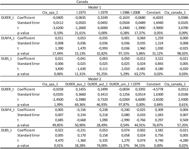
6.2.Results of Strategy 2
The results of a sequence of tests for assessing the existence of interdependence among different countries are reported in the following tables. Two models are estimated. The first one is a multivariate VECM model for each country, expanded with the cointegration vectors and for the remaining countries. Thereafter, I used a simplification algorithm available at Oxmetrics. The second model is a multivariate model that is expanded not only with the error correction mechanisms but also with the first difference of the logarithm of the exchange rate and the ratio of Net Foreign Asset Position (NFA) on GDP, which is the indicator of the Balassa-Samuelson effect. In this case, this second option not only tests the existence of interdependence of misalignments (imbalances) but also tests the short-run dynamics of a specific country in relation to the short-run dynamics of other countries.
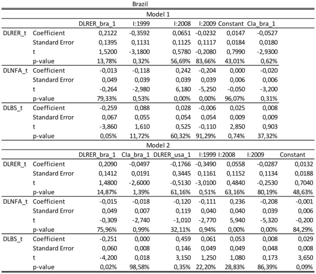
6.2.1.Brazil
Model 2 was obtained from the general model that contained not only the cointegration vectors of all the countries analyzed, but also the first difference from the logarithm of the variables collected for all countries. The final model suggests that the changes in the effective exchange rate in the United States influence the Brazilian economy. Either way, the dynamics of the Brazilian exchange rate do not appear to have been influenced directly by global factors. The only economy that appears to have influenced the Brazilian data is the US economy, and this was widely expected given the extent of trade and financial integration between the two countries.
DLRER_bra_1 I:1999 I:2008 I:2009 Constant CIa_bra_1 DLRER_t Coefficient 0,2122 -0,3592 0,0651 -0,0232 0,0147 -0,0527
Standard Error 0,1395 0,1131 0,1125 0,1117 0,0184 0,0180 t 1,5200 -3,1800 0,5780 -0,2080 0,7990 -2,9300 p-value 13,78% 0,32% 56,69% 83,66% 43,01% 0,62% DLNFA_t Coefficient -0,013 -0,118 0,242 -0,204 0,000 -0,020 Standard Error 0,049 0,039 0,039 0,039 0,006 0,006 t -0,264 -2,980 6,180 -5,250 -0,050 -3,200 p-value 79,33% 0,53% 0,00% 0,00% 96,07% 0,31% DLBS_t Coefficient -0,259 0,088 0,028 -0,006 0,025 0,008 Standard Error 0,067 0,055 0,054 0,054 0,009 0,009 t -3,860 1,610 0,525 -0,110 2,850 0,903 p-value 0,05% 11,72% 60,32% 91,29% 0,74% 37,32%
DLRER_bra_1 CIa_bra_1 DLRER_usa_1 I:1999 I:2008 I:2009 Constant DLRER_t Coefficient 0,2090 -0,0497 -0,1766 -0,3490 0,0558 -0,0287 0,0132
Standard Error 0,1412 0,0191 0,3445 0,1161 0,1152 0,1134 0,0188 t 1,4800 -2,6000 -0,5130 -3,0100 0,4840 -0,2530 0,7040 p-value 14,87% 1,39% 61,16% 0,51% 63,16% 80,19% 48,63% DLNFA_t Coefficient -0,015 -0,018 -0,120 -0,111 0,236 -0,208 -0,001 Standard Error 0,049 0,007 0,119 0,040 0,040 0,039 0,006 t -0,309 -2,740 -1,010 -2,770 5,940 -5,320 -0,200 p-value 75,96% 0,99% 32,11% 0,94% 0,00% 0,00% 84,29% DLBS_t Coefficient -0,251 0,000 0,459 0,061 0,053 0,008 0,029 Standard Error 0,060 0,008 0,146 0,049 0,049 0,048 0,008 t -4,200 0,018 3,150 1,250 1,080 0,173 3,650 p-value 0,02% 98,58% 0,35% 22,20% 28,83% 86,39% 0,09%
Brazil
Model 2 Model 1
Note: Cla denotes the cointegration vector.
6.2.2.The United States
Table 5 presents the results of the tests of interdependence applied to the United States. The results suggest that the misalignment of other countries does not influence the dynamics of the model that contains US series. This result contrasts with the conclusions reported in section 6.1.2. Only the model with an extended information set provides evidence in favor of interdependence. The change in the real exchange rate of the Netherlands appears to be linked to United States data. This result is not intuitive and could have been due to the casual retention of unimportant variables. The results for the United States suggest that the US economy is barely influenced by changes in the economies of the rest of the world.
DLRER_usa_1 I:1974 I:1986 I:2005 I:2008 I:2009 Constant CIa_eua_1 DLRER_t Coefficient 0,5442 0,0502 -0,1537 0,0146 -0,0201 0,0513 -0,2004 0,0121757
Standard Error 0,1269 0,0446 0,0469 0,0429 0,0431 0,0436 0,1036 0,006329
t 4,2900 1,1300 -3,2800 0,3390 -0,4660 1,1800 -1,9300 1,92
p-value 0,02% 26,89% 0,26% 73,68% 64,48% 24,85% 6,22% 0,0636
DLNFA_t Coefficient -0,011 -0,014 0,011 0,078 -0,095 0,061 -0,043 0,002
Standard Error 0,070 0,025 0,026 0,024 0,024 0,024 0,057 0,003
t -0,152 -0,551 0,423 3,270 -3,980 2,530 -0,744 0,626
p-value 87,98% 58,53% 67,50% 0,26% 0,04% 1,68% 46,24% 53,62%
DLBS_t Coefficient -0,175 0,358 0,109 0,038 0,020 -0,060 -0,203 0,012
Standard Error 0,151 0,053 0,056 0,051 0,051 0,052 0,124 0,008
t -1,150 6,720 1,950 0,745 0,386 -1,150 -1,640 1,550
p-value 25,75% 0,00% 5,98% 46,21% 70,20% 26,01% 11,04% 13,24%
DLRER_net_1 I:1974 I:1986 I:2008 Constant CIa_eua_1 DLRER_t Coefficient -0,9557 0,0370 -0,1691 -0,0418 -0,1534 0,0095 Standard Error 0,2112 0,0424 0,0458 0,0413 0,0986 0,0060
t -4,5300 0,8720 -3,7000 -1,0100 -1,5600 1,5900
p-value 0,01% 38,92% 0,08% 31,91% 12,93% 12,18%
DLNFA_t Coefficient 0,301 -0,026 0,022 -0,100 -0,076 0,004 Standard Error 0,136 0,027 0,029 0,027 0,064 0,004
t 2,210 -0,939 0,749 -3,760 -1,200 1,140
p-value 3,39% 35,47% 45,89% 0,07% 23,73% 26,30%
DLBS_t Coefficient 0,085 0,368 0,103 0,028 -0,188 0,011 Standard Error 0,265 0,053 0,057 0,052 0,124 0,008
t 0,322 6,920 1,790 0,548 -1,520 1,430
p-value 74,96% 0,00% 8,31% 58,75% 13,75% 16,30%
United States Model 1
Model 2
Note: Cla denotes the cointegration vector.
Table 4: Final model obtained from the selection made using the Ox algorithm: United States.
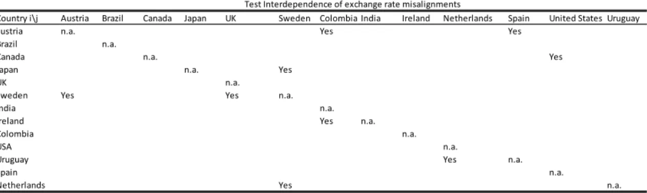
6.2.3.Other Countries
Country i\j Austria Brazil Canada Japan UK Sweden Colombia India Ireland Netherlands Spain United States Uruguay
austria n.a. Yes Yes
Brazil n.a.
Canada n.a. Yes
Japan n.a. Yes
UK n.a.
Sweden Yes Yes n.a.
India n.a.
Ireland Yes n.a.
Colombia n.a.
USA n.a.
Uruguay Yes n.a.
Spain n.a.
Netherlands Yes n.a.
n.a. - not applicable.
Test Interdependence of exchange rate misalignments
Table 5: Summary of the results of evaluating interdependence using exchange rate misalignment.
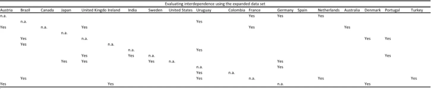
Table 6 presents the results of the strategy that contains the results of a data set that is expanded with not only misalignments but also the first differences of the various variables of other countries. In this case, the evidence for interdependence increases substantially. This finding suggests that in the long run, exchange rates would be simply explained by domestic fundamentals, while in the short run, events in larger economies like the United States or United Kingdom may generate a certain impact on other countries. There is also evidence of a strong regional interconnection among European countries, which was highly expected.
Austria Brazil Canada Japan United KingdomIreland India Sweden United States Uruguay Colombia France Germany Spain Netherlands Australia Denmark Portugal Turkey
n.a. Yes Yes Yes
n.a. Yes
Yes n.a. Yes Yes Yes
n.a.
Yes n.a. Yes Yes
Yes n.a.
n.a. Yes
Yes Yes n.a. Yes
Yes Yes Yes n.a. Yes
n.a. Yes
Yes n.a.
Yes Yes n.a. Yes Yes
Yes Yes n.a. Yes
cable.
Evaluating interdependence using the expanded data set
Table 6: Summary of the results of evaluating interdependence among countries using the Expanded Information data set.
Country i - Dummy 1973 1974 1975 1976 1977 1979 1980 1981 1983 1984 1985 1986 1993 1994 1999 2000 2001 2002 2003 2005 2006 2008 2009 2010
austria X X X X
Brazil X X X
Canada X
Japan X X X X X X
UK X X X X
Sweden X X X X
India
Ireland X X X X X
Colombia X X X X
USA X X X X X X
Uruguay X X X X X
Spain X X X X X
Netherlands X X X X
X - means significance.
Points of Instability in the global model extended by exchange rate misalignment
Table 7: Summary of identified points of instability in the estimated models using exchange rate
misalignment.
Table presents the results for the expanded data set. The results suggest a smaller number of points of instability, particularly in terms of the events after the 2008 crisis. This suggests that the expanded data set is the most appropriate for explaining the data of several countries. Further, the results may also suggest that the spread of events that followed the 2008 crisis follow a traditional mechanism.
Country i - Dummy 1973 1974 1975 1976 1977 1979 1980 1981 1983 1984 1985 1986 1993 1994 1999 2000 2001 2002 2003 2005 2008 2009 2010
Austria X
Brazil X X X
Canada X
Japan X X
UK X
Sweden X X X X
India X X
Ireland X X
Colombia X
USA X X X
Uruguay X X X X
Spain X
Netherlands X X X
X - means significance.
Points of Instability in the global model extended by misalignment and other variables
Table 8: Summary of identified points of instability in the estimated models—expanded by
6.3. Main findings
The following is a summary of the main conclusions of this study:
a) There is some evidence of interdependence among the analyzed countries in terms of exchange rate. The dynamics of the US data appear to affect a large number of countries. This is in line with the importance of this country in the global economy. b) There is evidence of strong interdependence among European nations.
c) A shock can only affect the exchange rates of a specific country if it permanently affects its fundamentals.
d) The mechanism of interdependence is restricted mainly to short-term dynamics. e) Since the error correction mechanisms of a particular country are not important in other countries, there is no reason for not employing Gonzalo and Granger’s decomposition methodology, which is a usual method for estimating exchange rate misalignment.
7.
Comparison with the results of existing literature
Dufrenot et al. (2006, 2008) do not use non-linear models for analyzing exchange rate misalignment, but the data set is restricted to data from the countries themselves. Pesaran and Smith (2006) and Pesaran et al. (2005) attempt to model the phenomena using a global model, although they do not apply the methodology to exchange rate misalignment. The authors seek to identify global factors and assess the extent to which such factors help to improve individual models.
Further, Groen and Kleibergen (2003) conduct a similar analysis to that of Larsson and Lyhagen (2007) and are able to detect interdependence between the dollar and other currencies, as expounded in the monetary approach (Dornbusch (1976) and Mussa (1974)). The hypothesis suggested by the monetary approach is not rejected in models in which panel data is used, which is in contrast with models that do not use panel data. In this regard, the results of the abovementioned studies are very close to those of the present study; the only difference lies in the fundamentals used.
Groen and Lombardelli (2004) is also similar to the current study, but their work is limited to model the relationship between the real exchange rate and the Balassa-Samuelson effect without considering the possible effect of the international investment position on the exchange rate.
8.
Conclusions
The objective of this study was to compare different methodologies for determining exchange rate misalignment and test the hypotheses that the exchange rates of different countries are influenced by their own fundamentals as well variables related to the fundamentals of other countries. The second hypothesis is related to the existence of interdependence among countries.
The methodology applied in this study differs from the traditional methodology of calculating exchange rate misalignment using models containing only variables of the particular country under study in that the methodology used in this study permits the expansion of the set of variables to include information related to other countries.
second strategy was to utilize a long panel data set that includes variables used to estimate exchange rate misalignment and formally test the hypothesis of no interdependence.
The results suggested that in both strategies there is some evidence of the existence of interdependence. The source of interdependence appears to be most related to short-term factors. However, it must be noted that the generation of long-term effects of the competitive devaluations in one country on the exchange rate of other countries would imply changing these fundamentals.
9.
References
Ahmad, Y. and W. D. Craighead (2010). "Temporal aggregation and purchasing power parity persistence." Journal of International Money and Finance, In Press, Accepted Manuscript.
Alberola, E., S. Cervero, et al. (1999). "Global equilibrium exchange rate: Euro, Dollar, 'Ins', 'Outs' and other major currencies in a panel cointegration framework." IMF Working Paper. Washington, IMF, 99-175.
Beveridge, S. and D. B. Nelson (1981). "A new approach to decomposition of economic time series into permanent and transitory components with particular attention to measurement of the business cycle." Journal of Monetary Economics 7(2): 151-174. Bilson, J. F. (1979). "Recent developments in monetary models of exchange rate determination." IMF Staff Paper 26(2): 201-223.
Camarero, M., J. Ordónez, et al. (2002). "The euro-dollar exchange rate: is it fundamental?" CESIFO Working Paper No. 798. Venice, CESIFO.
Cavaliere, G., A. Rahbek, et al. (2008). "Testing for co-Integration in vector autoregressions with non-stationary volatility." Journal of Econometrics 158(10): 23. Clark, P. B. and R. MacDonald (1998). Exchange rates and economic fundamentals: a methodological comparison of BEERs and FEERs, International Monetary Fund.
Dornbusch, R. (1976). "Expectations and exchange rate dynamics." Journal of Political Economy 84(6): 1161-1176.
Dufrenot, G., L. Mathieu, et al. (2006). "Persistent misalignments of the European exchange rates: some evidence from non-linear cointegration." Applied Economics 38: 203-229.
Dufrénot, G., S. Lardic, et al. (2008). "Explaining the European exchange rates deviations: long memory or non-linear adjustment?" Journal of International Financial Markets, Institutions and Money 18(3): 207-215.
Edwards, S. (1987). "Exchange rate misaligment in developing countries." NBER Working Paper No. 442.
Eichengreen, B. and J. D. Sachs (1986). Exchange rates and economic recovery in the 1930s, National Bureau of Economic Research Cambridge, Mass., USA.
Engle, R. F. and C. W. J. Granger (1987). "Co-integration and error correction: representation, estimation and testing." Econometrica 55: 251-276.
Faruqee, H. (1995). "Long-run determinants of the real exchange rate: A stock flow Perspective." IMF Staff Paper 42: 80-107.
Froot, K. A. and K. Rogoff, Eds. (1995). Perspectives on PPP and long-run real exchange rates. Handbook of International Economics. Amsterdam, North-Holland. Glick, R. and A. K. Rose (1998). "Contagion and trade: why are currency crises regional? NBER Working Paper No. 6806, Washington, NBER.
Gonzalo, J. and C. W. J. Granger (1995). "Estimation of common long-memory components in cointegrated systems." Journal of Business and Economics Statistics 13(1).
Gredenhoff, M. and T. Jacobson (2001). "Bootstrap testing linear restrictions on cointegrating vectors." Journal of Business & Economic Statistics 19(1): 63-72.
Groen, J. and C. Lombardelli (2004). "Real exchange rates and the relative prices of non-traded and traded goods: an empirical analysis." Bank of England Working Paper No. 223.
Groen, J. J. J. and F. Kleibergen (2003). "Likelihood-based cointegration analysis in panels of vector error-correction models. 21: 295-318.
Hansen, P. R. (2003). "Structural changes in the cointegrated vector autoregressive model." Journal of Econometrics 114: 261-295.
Hendry, D. and H. M. Krolzig (2005). "The properties of automatic GETS modelling." Economic Journal 115: 32-61.
Hendry, D. F. and J. A. Doornik (2006). Modelling dynamic systems using PcGive. London.
Johansen, S. (1988). "Statistical analysis of cointegration vectors." Journal of Economic Dynamics and Control 12(2): 231-254.
Johansen, S. (1995). Likelihood-based Inference in cointegrated vector autoregressive models. Oxford, Oxford University Press.
Johansen, S. (1999). A Bartlett correction factor for tests on the cointegrating relations. Florence, European University Institute.
Johansen, S. (2000). A small sample correction of the test for cointegrating rank in the vector autoregressive model. Florence, European University Institute.
Juselius, K. (2009). The cointegrated VAR model methodology and applications Oxford, Oxford University Press.
Kubota, M. (2009). "Real exchange rate misalignments: theoretical modelling and empirical evidence." Discussion Papers in Economics, York, University of York.
Kubota, M. (2009). "Real exchange rate misaligments." Department of Economics, York, University of York. Phd: 201.
Lane, P. R. and G. M. Milesi-Ferretti (2007). "The external wealth of nations mark II: revised and extended estimates of foreign assets and liabilities, 1970-2004." Journal of International Economics 73(2): 223-250.
Larsson, R., J. Lyhagen, et al. (2001). "Likelihood-based cointegration tests in heterogeneous panels." Econometric Journal 4: 109-142.
Larsson, R. and J. Lyhagen (2007). "Inference in panel cointegration models with long panels." Journal of Business and Economic Statistics 25(4): 473-483.
Lutkepohl, H. (2007). New introduction to multiple time series analysis, Springer. Meese, R. A. and K. Rogoff (1983). "Empirical exchange models of the seventies: do they fi out of the sample?" Journal of International Economics 14: 3-24.
Mussa, M. (1974). "A monetary approach to balance-of-payments analysis." Journal of Money, Credit and Banking 6(3): 333-351.
Pesaran, M. H., Y. Shin, et al. (1999). "Pooled mean group estimation of dynamic heterogeneous panels." Journal of American Statistical Association 94(446): 621-634. Pesaran, M. H., L. V. Smith, et al. (2005). What if the UK had joined the Euro in 1999? : an empirical evaluation using a global VAR. Cambridge, University of Cambridge Faculty of Economics.
Pesaran, M. H. and R. Smith (2006). Macroeconomic modelling with a global perspective. Cambridge, Faculty of Economics University of Cambridge.
Santos, C., D. Hendry, et al. (2008). "Automatic selection of indicators in a fully saturated regression." Computational Statistics 23(2): 317-335.
Shin, Y. (1994). "A residual-based test of the null of cointegration against the alternative of no cointegration." Econometric Theory 10(1): 91-115.
Stein, J. (1995). "The fundamental determinants of the real exchange rate of the U.S. dollar relative to other G-7 currencies." IMF Working Paper Nos. 95-81.
Swensen, A. R. (2006). "Bootstrap algorithms for testing and determining the cointegration rank in VAR models." Econometrica 74(6): 1699-1714.
Taylor, A. M. (2001). "Potential pitfalls for the purchasing-power-parity puzzle? Sampling and specification biases in mean-reversion tests of the law of one price." Econometrica 69(2): 473-498.
Turnovsky, S. J., T. Basar, et al. (1987). "Dynamic strategic monetary policies and coordination in interdependent economies. NBER Working Paper No. 2467, Washington.
Ugai, H. (2007). "Effects of the quantitative easing policy: A survey of empirical analyses." Monetary and Economic Studies—Bank of Japan 25(1): 1.
Appendix
CIa_spa_1 I:1973 I:1979 I:1986 I:2008 Constant CIa_canada_1
DLRER_t Coefficient -0,0405 -0,0635 0,3249 -0,1633 -0,0680 -6,6033 0,0386
Standard Error 0,0112 0,0503 0,0492 0,0504 0,0489 1,6940 0,0105
t -3,6200 -1,2600 6,6000 -3,2400 -1,3900 -3,9000 3,6700
p-value 0,10% 21,61% 0,00% 0,28% 17,37% 0,05% 0,09%
DLNFA_t Coefficient 0,011 0,053 -0,035 0,001 0,069 1,259 0,000
Standard Error 0,008 0,036 0,036 0,036 0,035 1,224 0,008
t 1,390 1,470 -0,993 0,036 1,960 1,030 -0,025
p-value 17,44% 15,13% 32,82% 97,15% 5,86% 31,12% 98,02%
DLBS_t Coefficient 0,021 -0,041 0,003 0,050 -0,012 3,522 -0,021
Standard Error 0,006 0,025 0,025 0,025 0,024 0,843 0,005
t 3,830 -1,630 0,111 2,010 -0,482 4,180 -4,020
p-value 0,06% 11,31% 91,25% 5,29% 63,27% 0,02% 0,03%
CIa_spa_1 DLRER_aus_1 DLRER_aut_1 DLRER_uni_1 I:1979 Constant CIa_canada_1
DLRER_t Coefficient -0,0258 0,1455 0,2499 -0,0034 0,3392 -4,5778 0,0312
Standard Error 0,0105 0,3660 0,3413 0,1256 0,0514 1,6300 0,0106
t -2,4500 0,3980 0,7320 -0,0269 6,6000 -2,8100 2,9300
p-value 1,99% 69,36% 46,93% 97,87% 0,00% 0,84% 0,61%
DLNFA_t Coefficient 0,005 -0,156 0,238 -0,240 -0,025 0,309 0,004
Standard Error 0,007 0,234 0,218 0,080 0,033 1,043 0,007
t 0,685 -0,668 1,090 -2,990 -0,766 0,297 0,569
p-value 49,85% 50,90% 28,49% 0,54% 44,91% 76,87% 57,35%
DLBS_t Coefficient 0,022 -0,231 0,053 0,074 0,002 3,582 -0,021
Standard Error 0,005 0,170 0,158 0,058 0,024 0,756 0,005
t 4,470 -1,360 0,335 1,270 0,074 4,740 -4,280
p-value 0,01% 18,28% 74,00% 21,37% 94,15% 0,00% 0,02%
Canada Model 1
Model 2
Note: Cla denotes the cointegration vector
CIa_india_1 CIa_uru_1 I:1973 I:1985 I:1986 I:2009 Constant CIa_austria_1 DLRER_t Coefficient -0,0268 -0,0081 0,0712 -0,2013 -0,1515 -0,0859 1,8263 0,0175
Standard Error 0,0088 0,0115 0,0517 0,0582 0,0601 0,0535 0,8268 0,0099
t -3,0600 -0,7050 1,3800 -3,4600 -2,5200 -1,6100 2,2100 1,7700
p-value 0,46% 48,59% 17,84% 0,16% 1,71% 11,85% 3,47% 8,65%
DLNFA_t Coefficient 0,007 -0,002 0,005 -0,033 -0,002 0,087 -1,647 -0,020
Standard Error 0,006 0,008 0,035 0,039 0,041 0,036 0,558 0,007
t 1,130 -0,281 0,157 -0,843 -0,057 2,400 -2,950 -3,050
p-value 26,67% 78,04% 87,64% 40,54% 95,46% 2,25% 0,60% 0,47%
DLBS_t Coefficient -0,003 0,006 -0,071 0,016 -0,015 -0,047 0,537 0,006
Standard Error 0,002 0,002 0,011 0,012 0,012 0,011 0,168 0,002
t -1,970 2,350 -6,740 1,350 -1,190 -4,330 3,190 3,070
p-value 5,83% 2,52% 0,00% 18,54% 24,18% 0,01% 0,32% 0,44%
DLpreco_relativDLRER_net_1 Dnfa_spa_1 I:1973 Constant CIa_austria_1 DLRER_t Coefficient -0,7996 0,8636 -0,4571 0,0417 -0,3130 -0,0042
Standard Error 0,6591 0,2869 0,1603 0,0584 0,7003 0,0095
t -1,2100 3,0100 -2,8500 0,7140 -0,4470 -0,4370
p-value 23,37% 0,50% 0,75% 48,02% 65,79% 66,46%
DLNFA_t Coefficient 0,3231 0,2349 -0,0607 0,0124 -1,1899 -0,0160 Standard Error 0,4181 0,1820 0,1017 0,0370 0,4442 0,0060
t 0,7730 1,2900 -0,5970 0,3350 -2,6800 -2,6600
p-value 44,52% 20,57% 55,45% 74,00% 1,14% 1,19%
DLBS_t Coefficient 0,273 0,060 -0,121 -0,059 0,240 0,003 Standard Error 0,139 0,061 0,034 0,012 0,148 0,002
t 1,960 0,987 -3,570 -4,820 1,620 1,680
p-value 5,82% 33,06% 0,11% 0,00% 11,38% 10,27%
Austria Model 1
Model 2
Note: Cla denotes the cointegration vector
Dnfa_col_1 CIa_uni_1 I:1974 I:1977 I:1986 I:2001 Constante CIa_col_1 DLRER_t Coefficient -0,613 0,013 0,089 0,191 -0,189 -0,009 1,321 -0,042
Standard Error 0,249 0,009 0,058 0,059 0,062 0,061 0,246 0,008
t -2,460 1,430 1,540 3,250 -3,070 -0,152 5,370 -5,400
p-value 0,020 0,163 0,135 0,003 0,004 0,880 0,000 0,000
DLNFA_t Coefficient 0,778 0,011 -0,013 -0,035 0,026 -0,109 -0,423 0,013
Standard Error 0,176 0,007 0,041 0,042 0,044 0,043 0,174 0,005
t 4,410 1,640 -0,313 -0,841 0,606 -2,510 -2,430 2,450
p-value 0,000 0,111 0,756 0,407 0,549 0,018 0,021 0,020
DLBS_t Coefficient 0,024 -0,011 0,069 -0,036 0,018 0,039 -0,379 0,012
Standard Error 0,103 0,004 0,024 0,024 0,026 0,025 0,102 0,003
t 0,228 -2,880 2,860 -1,480 0,722 1,520 -3,710 3,710
p-value 82,08% 0,72% 0,75% 14,77% 47,56% 13,86% 0,08% 0,08%
Dnfa_col_1o_relativo_jap_1 Dnfa_ire_1 Dnfa_net_1 Dnfa_spa_1I:1974 Constante CIa_col_1 DLRER_t Coefficient -0,2543 -0,2278 0,0522 0,1370 -0,3956 0,0687 1,4490 -0,0461
Standard Error 0,2792 0,2027 0,0682 0,1195 0,2023 0,0702 0,2853 0,0089
t -0,9110 -1,1200 0,7650 1,1500 -1,9600 0,9780 5,0800 -5,1800
p-value 36,95% 26,96% 44,99% 26,04% 5,96% 33,56% 0,00% 0,00%
DLNFA_t Coefficient 0,595 -0,276 0,133 0,164 -0,131 -0,025 -0,250 0,008
Standard Error 0,126 0,092 0,031 0,054 0,092 0,032 0,129 0,004
t 4,710 -3,010 4,290 3,030 -1,440 -0,782 -1,940 1,900
p-value 0,00% 0,52% 0,02% 0,49% 16,11% 44,02% 6,21% 6,70%
DLBS_t Coefficient -0,089 -0,066 -0,057 -0,061 0,266 0,066 -0,420 0,013
Standard Error 0,084 0,061 0,021 0,036 0,061 0,021 0,086 0,003
t -1,060 -1,080 -2,740 -1,690 4,360 3,110 -4,880 4,940
p-value 29,88% 28,79% 1,00% 10,09% 0,01% 0,40% 0,00% 0,00%
Colombia Model 1
Model 2
Note: Cla denotes the cointegration vector.
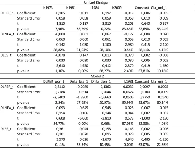
I:1973 I:1981 I:1984 I:2009 Constant CIa_uni_1
DLRER_t Coefficient -0,105 0,011 0,197 -0,012 0,006 0,005
Standard Error 0,058 0,058 0,059 0,058 0,010 0,009
t -1,810 0,187 3,310 -0,205 0,640 0,597
p-value 7,96% 85,29% 0,22% 83,85% 52,69% 55,44%
DLNFA_t Coefficient -0,008 0,061 0,067 -0,177 -0,004 0,020
Standard Error 0,060 0,060 0,061 0,059 0,010 0,009
t -0,142 1,030 1,100 -2,980 -0,415 2,120
p-value 88,82% 31,04% 28,10% 0,54% 68,11% 4,16%
DLBS_t Coefficient -0,078 0,147 0,013 0,070 0,002 -0,008
Standard Error 0,030 0,030 0,030 0,030 0,005 0,005
t -2,610 4,950 0,412 2,370 0,419 -1,680
p-value 1,36% 0,00% 68,27% 2,40% 67,81% 10,16%
DLRER_por_1 Dnfa_bra_1 Dnfa_den_1 I:1981 Constant CIa_uni_1
DLRER_t Coefficient -0,5112 -0,2089 -0,1362 0,0032 0,0097 0,0025
Standard Error 0,2184 0,1514 0,2044 0,0624 0,0100 0,0099
t -2,3400 -1,3800 -0,6660 0,0506 0,9750 0,2540
p-value 2,54% 17,68% 50,97% 95,99% 33,67% 80,14%
DLNFA_t Coefficient 0,093 -0,645 -0,548 0,025 -0,007 0,015
Standard Error 0,154 0,106 0,144 0,044 0,007 0,007
t 0,608 -6,060 -3,810 0,573 -1,000 2,130
p-value 54,77% 0,00% 0,06% 57,05% 32,38% 4,08%
DLBS_t Coefficient 0,361 0,044 -0,158 0,143 0,002 -0,006
Standard Error 0,101 0,070 0,095 0,029 0,005 0,005
t 3,570 0,626 -1,670 4,940 0,485 -1,230
p-value 0,11% 53,54% 10,45% 0,00% 63,07% 22,66%
United Kindgom
Model 2
Note: Cla denotes the cointegration vector.
Table 12: Final model selected using the Ox algorithm: United Kingdom.
Dnfa_ind_1 I:1974 I:1976 I:1993 I:2009 Constant UCIa_india_1 U DLRER_t Coeficiente 0,726 0,135 -0,117 0,124 -0,074 0,539 -0,0284
Erro Padrão 0,435 0,057 0,056 0,061 0,059 0,174 0,0087 t 1,670 2,380 -2,080 2,030 -1,250 3,100 -3,2700 p-valor 10,49% 2,35% 4,60% 5,11% 22,18% 0,40% 0,26% DLNFA_t Coeficiente 0,720 -0,006 0,027 0,063 -0,009 -0,011 0,000 Erro Padrão 0,132 0,017 0,017 0,019 0,018 0,053 0,003 t 5,460 -0,367 1,580 3,380 -0,473 -0,216 0,186 p-valor 0,00% 71,58% 12,47% 0,19% 63,97% 83,07% 85,34% DLBS_t Coeficiente -0,041 -0,074 -0,020 -0,021 0,056 -0,162 0,008 Erro Padrão 0,109 0,014 0,014 0,015 0,015 0,043 0,002 t -0,374 -5,240 -1,410 -1,360 3,790 -3,720 3,880 p-valor 71,08% 0,00% 16,88% 18,31% 0,06% 0,08% 0,05%
Dnfa_ind_1 reco_relativo_usa Dnfa_usa_1 I:1974 I:1976 Constant CIa_india_1 DLRER_t Coeficiente 0,6724 -0,2451 0,4215 0,1345 -0,1429 0,3377 -0,0181
Erro Padrão 0,4217 0,1161 0,2970 0,0560 0,0559 0,1555 0,0078 t 1,5900 -2,1100 1,4200 2,4000 -2,5600 2,1700 -2,3300 p-valor 12,06% 4,27% 16,56% 2,23% 1,55% 3,74% 2,61% DLNFA_t Coeficiente 0,673 -0,049 -0,031 -0,010 0,022 -0,070 0,004 Erro Padrão 0,149 0,041 0,105 0,020 0,020 0,055 0,003 t 4,530 -1,210 -0,297 -0,492 1,120 -1,290 1,290 p-valor 0,01% 23,63% 76,86% 62,59% 26,91% 20,78% 20,78% DLBS_t Coeficiente -0,040 0,071 -0,355 -0,078 -0,008 -0,074 0,004 Erro Padrão 0,082 0,022 0,057 0,011 0,011 0,030 0,002 t -0,486 3,160 -6,180 -7,250 -0,710 -2,460 2,640 p-valor 63,03% 0,34% 0,00% 0,00% 48,27% 1,96% 1,27%
India Modelo 1
Modelo 2
Table 13: Final model selected using the Ox algorithm: India
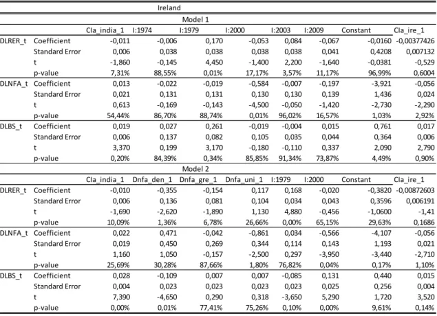
CIa_india_1 I:1974 I:1979 I:2000 I:2003 I:2009 Constant CIa_ire_1 DLRER_t Coefficient -0,011 -0,006 0,170 -0,053 0,084 -0,067 -0,0160 -0,00377426
Standard Error 0,006 0,038 0,038 0,038 0,038 0,041 0,4208 0,007132
t -1,860 -0,145 4,450 -1,400 2,200 -1,640 -0,0381 -0,529
p-value 7,31% 88,55% 0,01% 17,17% 3,57% 11,17% 96,99% 0,6004
DLNFA_t Coefficient 0,013 -0,022 -0,019 -0,584 -0,007 -0,197 -3,921 -0,056
Standard Error 0,021 0,131 0,131 0,130 0,130 0,139 1,436 0,024
t 0,613 -0,169 -0,143 -4,500 -0,050 -1,420 -2,730 -2,290
p-value 54,44% 86,70% 88,74% 0,01% 96,02% 16,57% 1,03% 2,92%
DLBS_t Coefficient 0,019 0,027 0,261 -0,019 -0,004 0,015 0,761 0,017
Standard Error 0,006 0,137 0,082 0,105 0,035 0,044 0,364 0,006
t 3,370 0,199 3,170 -0,180 -0,110 0,337 2,090 2,790
p-value 0,20% 84,39% 0,34% 85,85% 91,34% 73,87% 4,49% 0,90%
CIa_india_1 Dnfa_den_1 Dnfa_gre_1 Dnfa_uni_1 I:1979 I:2000 Constant CIa_ire_1 DLRER_t Coefficient -0,010 -0,355 -0,154 0,117 0,168 -0,020 -0,3820 -0,00872603
Standard Error 0,006 0,136 0,081 0,104 0,034 0,043 0,3596 0,006191
t -1,690 -2,620 -1,890 1,130 4,880 -0,456 -1,0600 -1,41
p-value 10,09% 1,36% 6,78% 26,66% 0,00% 65,15% 29,63% 0,1686
DLNFA_t Coefficient 0,022 0,471 -0,042 -0,861 0,034 -0,566 -4,107 -0,056
Standard Error 0,019 0,450 0,269 0,344 0,114 0,143 1,193 0,021
t 1,160 1,050 -0,157 -2,500 0,297 -3,950 -3,440 -2,710
p-value 25,69% 30,28% 87,66% 1,80% 76,82% 0,04% 0,17% 1,10%
DLBS_t Coefficient 0,028 -0,109 0,007 0,007 -0,085 0,131 0,440 0,015
Standard Error 0,004 0,023 0,023 0,023 0,023 0,025 0,256 0,004
t 7,390 -4,650 0,290 0,318 -3,650 5,290 1,720 3,520
p-value 0,00% 0,01% 77,41% 75,26% 0,10% 0,00% 9,61% 0,14%
Ireland Model 1
Model 2
Note: Cla denotes the cointegration vector.
CIa_swe_1 I:1975 I:1999 I:2005 I:2010 Constant CIa_jap_1
DLRER_t Coefficient 0,0366 -0,0370 0,1298 -0,0916 -0,0024 2,7562 -0,0093
Standard Error 0,0151 0,0938 0,0933 0,0946 0,1027 1,1780 0,0153
t 2,4200 -0,3940 1,3900 -0,9690 -0,0237 2,3400 -0,6050
p-value 2,14% 69,63% 17,38% 33,98% 98,13% 2,57% 54,92%
DLNFA_t Coefficient -0,014 0,045 -0,153 -0,088 -0,083 -0,806 -0,012
Standard Error 0,004 0,024 0,024 0,024 0,027 0,305 0,004
t -3,630 1,860 -6,350 -3,620 -3,120 -2,650 -3,020
p-value 0,10% 7,28% 0,00% 0,10% 0,38% 1,25% 0,49%
DLBS_t Coefficient -0,021 -0,119 -0,087 0,056 0,253 -1,707 0,013
Standard Error 0,008 0,052 0,051 0,052 0,057 0,649 0,008
t -2,510 -2,310 -1,700 1,080 4,470 -2,630 1,520
p-value 1,74% 2,77% 9,95% 28,72% 0,01% 1,30% 13,78%
DLpreco_relativ I:1999 I:2010 Constant CIa_jap_1
DLRER_t Coefficient -0,1842 0,0926 0,0111 -0,0954 0,0073
Standard Error 0,2031 0,0966 0,1069 0,2191 0,0143
t -0,9070 0,9580 0,1030 -0,4350 0,5070
p-value 37,07% 34,48% 91,82% 66,60% 61,57%
DLNFA_t Coefficient 0,033 -0,133 -0,068 0,207 -0,012
Standard Error 0,068 0,032 0,036 0,073 0,005
t 0,480 -4,130 -1,920 2,830 -2,610
p-value 63,40% 0,02% 6,34% 0,77% 1,32%
DLBS_t Coefficient -0,158 -0,067 0,227 -0,043 0,001
Standard Error 0,118 0,056 0,062 0,128 0,008
t -1,330 -1,190 3,640 -0,333 0,103
p-value 19,19% 24,20% 0,09% 74,13% 91,82%
Japan Model 1
Model 2
Note: Cla denotes the cointegration vector.
DLpreco_relativo_net_1 CIa_swe_1 I:1984 I:1985 I:1999 I:2003 Constant UCIa_net_1 DLRER_t Coefficient 0,2716 0,0125 -0,0353 -0,0017 -0,0019 0,0623 0,9294 0,0102378
Standard Error 0,1346 0,0050 0,0263 0,0314 0,0271 0,0268 0,3468 0,004584 t 2,0200 2,4900 -1,3400 -0,0529 -0,0714 2,3200 2,6800 2,23 p-value 5,23% 1,83% 18,93% 95,82% 94,35% 2,68% 1,17% 0,0329 DLNFA_t Coefficient -0,009 0,016 0,033 0,040 0,338 0,278 1,041 -0,020 Standard Error 0,403 0,015 0,079 0,094 0,081 0,080 1,039 0,014
t -0,022 1,070 0,413 0,429 4,170 3,460 1,000 -1,480
p-value 98,30% 29,40% 68,21% 67,06% 0,02% 0,16% 32,43% 14,78% DLBS_t Coefficient 0,236 -0,011 -0,108 0,167 -0,001 -0,003 -0,763 -0,002 Standard Error 0,110 0,004 0,022 0,026 0,022 0,022 0,284 0,004 t 2,140 -2,590 -5,020 6,510 -0,026 -0,124 -2,680 -0,525 p-value 4,02% 1,44% 0,00% 0,00% 97,98% 90,23% 1,16% 60,30% DLRER_por_1 Dnfa_aus_1 Dnfa_swe_1 I:1985 I:1994 I:1999 Constant U CIa_net_1 DLRER_t Coefficient -0,0537 -0,1940 -0,0863 -0,0546 -0,0184 -0,0124 0,0735 0,0169529
Standard Error 0,1103 0,1439 0,0497 0,0315 0,0311 0,0309 0,0204 0,004875 t -0,4870 -1,3500 -1,7400 -1,7300 -0,5920 -0,4020 3,6100 3,48 p-value 62,97% 18,72% 9,23% 9,33% 55,85% 69,04% 0,11% 0,0015 DLNFA_t Coefficient 0,152 1,029 -0,373 0,097 -0,310 0,418 -0,046 -0,0103384 Standard Error 0,172 0,225 0,078 0,049 0,049 0,048 0,032 0,007611
t 0,884 4,580 -4,810 1,970 -6,380 8,650 -1,440 -1,36
p-value 38,35% 0,01% 0,00% 5,78% 0,00% 0,00% 15,91% 0,1841 DLBS_t Coefficient 0,368 -0,391 -0,035 0,123 -0,006 0,005 -0,053 -0,0129943 Standard Error 0,093 0,121 0,042 0,027 0,026 0,026 0,017 0,004114
t 3,960 -3,220 -0,841 4,610 -0,245 0,206 -3,100 -3,16
p-value 0,04% 0,30% 40,70% 0,01% 80,77% 83,78% 0,41% 0,35% Netherlands
Model 1
Model 2
Note: Cla denotes the cointegration vector.