❊♥s❛✐♦s ❊❝♦♥ô♠✐❝♦s
❊s❝♦❧❛ ❞❡
Pós✲●r❛❞✉❛çã♦
❡♠ ❊❝♦♥♦♠✐❛
❞❛ ❋✉♥❞❛çã♦
●❡t✉❧✐♦ ❱❛r❣❛s
◆◦ ✹✼✵ ■❙❙◆ ✵✶✵✹✲✽✾✶✵
❚❤❡ ❆❧✐❛s✐♥❣ ❊✛❡❝t✱ t❤❡ ❋❡❥❡r ❑❡r♥❡❧ ❛♥❞
❚❡♠♣♦r❛❧❧② ❆❣❣r❡❣❛t❡❞ ▲♦♥❣ ▼❡♠♦r② Pr♦✲
❝❡ss❡s
▲❡♦♥❛r❞♦ ❘♦❝❤❛ ❙♦✉③❛
❖s ❛rt✐❣♦s ♣✉❜❧✐❝❛❞♦s sã♦ ❞❡ ✐♥t❡✐r❛ r❡s♣♦♥s❛❜✐❧✐❞❛❞❡ ❞❡ s❡✉s ❛✉t♦r❡s✳ ❆s
♦♣✐♥✐õ❡s ♥❡❧❡s ❡♠✐t✐❞❛s ♥ã♦ ❡①♣r✐♠❡♠✱ ♥❡❝❡ss❛r✐❛♠❡♥t❡✱ ♦ ♣♦♥t♦ ❞❡ ✈✐st❛ ❞❛
❋✉♥❞❛çã♦ ●❡t✉❧✐♦ ❱❛r❣❛s✳
❊❙❈❖▲❆ ❉❊ PÓ❙✲●❘❆❉❯❆➬➹❖ ❊▼ ❊❈❖◆❖▼■❆ ❉✐r❡t♦r ●❡r❛❧✿ ❘❡♥❛t♦ ❋r❛❣❡❧❧✐ ❈❛r❞♦s♦
❉✐r❡t♦r ❞❡ ❊♥s✐♥♦✿ ▲✉✐s ❍❡♥r✐q✉❡ ❇❡rt♦❧✐♥♦ ❇r❛✐❞♦ ❉✐r❡t♦r ❞❡ P❡sq✉✐s❛✿ ❏♦ã♦ ❱✐❝t♦r ■ss❧❡r
❉✐r❡t♦r ❞❡ P✉❜❧✐❝❛çõ❡s ❈✐❡♥tí✜❝❛s✿ ❘✐❝❛r❞♦ ❞❡ ❖❧✐✈❡✐r❛ ❈❛✈❛❧❝❛♥t✐
❘♦❝❤❛ ❙♦✉③❛✱ ▲❡♦♥❛r❞♦
❚❤❡ ❆❧✐❛s✐♥❣ ❊❢❢❡❝t✱ t❤❡ ❋❡❥❡r ❑❡r♥❡❧ ❛♥❞ ❚❡♠♣♦r❛❧❧② ❆❣❣r❡❣❛t❡❞ ▲♦♥❣ ▼❡♠♦r② Pr♦❝❡ss❡s✴ ▲❡♦♥❛r❞♦ ❘♦❝❤❛ ❙♦✉③❛ ✕ ❘✐♦ ❞❡ ❏❛♥❡✐r♦ ✿ ❋●❱✱❊P●❊✱ ✷✵✶✵
✭❊♥s❛✐♦s ❊❝♦♥ô♠✐❝♦s❀ ✹✼✵✮ ■♥❝❧✉✐ ❜✐❜❧✐♦❣r❛❢✐❛✳
The Aliasing Effect, the Fejer Kernel and Temporally Aggregated Long
Memory Processes
Leonardo R. Souza EPGE – Fundação Getúlio Vargas
January 2003
Abstract
This paper derives the spectral density function of aggregated long memory processes in light of the aliasing effect. The results are different from previous analyses in the literature and a small simulation exercise provides evidence in our favour. The main result point to that flow aggregates from long memory processes shall be less biased than stock ones, although both retain the degree of long memory. This result is illustrated with the daily US Dollar/ French Franc exchange rate series.
Keywords: TemporalAggregation, Long Memory, Aliasing, Fejer Kernel JEL classification: C14, C22, C43
1 - Introduction
Temporally aggregated time series data appear frequently in Economics, either because the collecting process implicitly aggregates data from different time periods or because the econometrician wants to work on a time frequency different (lower) than that of the collected data. Temporal aggregation has distinct interpretations depending on the underlying variable be a stock or a flow variable. A stock variable is aggregated through skip-sampling while a flow variable is aggregated by summing subsequent observations letting no overlap in the sums.
example. If the time unit is small, high frequency data are collected and the sample size usually remains big after aggregation. However, if the original data are, e.g., monthly and aggregated to quarterly series, a small aggregated series is usually obtained. An example of high frequency series whose memory parameter (or alternatively integration order) is estimated across different levels of aggregation is the French Franc/German Mark exchange rate that appears in Bisaglia and Guégan (1998). As to low frequency data, Diebold and Rudebusch (1989) use annual and quarterly data in their (long memory) study of real US GNP and Chambers (1998) uses quarterly and annual flow data to estimate the memory parameter of a number of UK macroeconomic series. Tschernig (1995), in turn, uses daily, weekly, monthly and quarterly data to investigate the long memory in many exchange rates.
Specification (and identification) of aggregated long memory processes is important since it can shed a light on the question of which data (aggregated or disaggregated) is preferable to use. Tschernig (1995) and Teles, Wei and Crato (1999) studied the effects of temporal aggregation (the latter only for the flow type) on AutoRegressive Fractionally Integrated Moving Average (ARFIMA) models. They conclude that an ARFIMA(p,d,q) turns out to be an ARFIMA(p,d,∞) when aggregated. They do not provide, however, the MA polynomial form for non-overlapping aggregates1. Crato and Ray (2002) provide the spectral density function of aggregated (flow) ARFIMA processes, but it depends on the MA(∞) polynomial that is not derived completely in Tschernig (1995) and Teles, Wei and Crato (1999). Chambers (1998) investigates the spectral density function of stock and flow aggregated long memory processes, as well as continuous-time long memory processes observed at discrete-time intervals and cross-sectionally aggregated long memory processes. For the temporal aggregation of discrete-time processes, however, he does not take into account the aliasing effect as he does in the case of the continuous-time processes. All these papers agree that neither type of aggregation changes the memory parameter.
and relates it to the aliasing effect. In contrast, the latter finds that temporal aggregation of flow processes generally does not induce any significant bias.
The issue of forecasting aggregated versus disaggregated long memory series is investigated in Souza and Smith (2002b). They compare the forecasting performance of aggregated (flow) ARFIMA series against the cumulative forecasts from the original series. They conclude that in general disaggregated models forecast better for d>0 and worse for d<0, comparing with aggregated models. This latter finding contrasts with the results from ARIMA models, where forecasts from the aggregated series are, at best, not much worse than aggregated forecasts from the underlying series (see Amemiya and Wu (1972), Lütkepohl (1986), Wei (1989) and Hotta and Neto (1993) to name a few).
The present paper is inserted among those on the issues of identification and estimation. It derives the spectral density function (alternatively speaking, spectral function, spectral density or spectrum) of aggregated stock and flow long memory processes in light of the Aliasing Theorem, unlike the previous works of Chambers (1998) and Crato and Ray (2002). The result is a completely different formula which a simulation study brings evidence in favour, as it matches with the periodogram averaged across 100 realizations of each process. The Aliasing Theorem is adapted to the case a discrete-time process is observed at a slower sampling rate. One may infer from the formulas that flow aggregates from long memory processes shall be less biased than stock ones. This result is illustrated with the daily US Dollar/ French Franc exchange rate from October 20, 1977 to October 23, 2002. In a long memory stochastic volatility model framework, the logarithm of the squared returns are analysed and the absence of long memory is rejected by the Lo’s (1991) modified R/S test. The series is aggregated as flow and stock variables and flow aggregates yield estimates of the same order as the original series, while stock aggregates yields estimates somewhat lower. This result is also consistent with the aforementioned works of Souza and Smith (2002a, b).
A secondary result is related with two conditions usually taken as equivalent; the time-domain condition:
∞ →
− ask
) (
~ 2d 1
k cρ k k
ρ (1)
1 They provide the MA(∞) polynomial (or an insight to it) for the overlapping type of aggregation,
and the frequency-domain condition: 0
as )
( ~ )
(λ cf λ λ −2d λ→
f (2)
where ρk and f(λ) are respectively the k-th order autocorrelation and the spectral density function of the process; c kρ( ) and cf(λ) are functions slowly varying as k tends to infinity and λ to zero, c kρ( ) having the same sign as d and cf(λ)being always positive; λ∈(−π,π]; and d is a real number. Stationarity holds for d < 0.5 so that it must apply in (1) and (2) in order to ρk and f(λ) have the usual meaning. The result is that a negative memory parameter d, according to its frequency-domain condition, changes with the aggregation of stock variables while remains unchanged if taken as to the time-domain condition. This proves the non-equivalence for d < 0 of the time- and frequency-domain conditions usually considered in the literature to define the memory parameter, given respectively by equations (1) and (2). On the other hand, aggregating a flow variable does not change the memory parameter according to either definition.
The plan of the paper is as follows. Section 2 defines long memory and ARFIMA models. Section 3 derives the autocovariances and the spectral density function of aggregated long memory processes, while Section 4 provides a small Monte Carlo simulation. An example with the daily US Dollar/ French Franc exchange rate series illustrates the results in Section 5. Section 6 offers a final consideration. All technical details and proofs are relegated to the Appendix.
2 – Long Memory Models
Long memory in stationary processes has traditionally two alternative definitions, one in the frequency-domain and the other in the time-domain2. Although there are some works in the literature that state they are equivalent, Robinson (1995, p.1632) argues that this is true only if the autocovariances are quasimonotonically convergent to zero. The time- and frequency-domain definitions of stationary long memory processes are respectively as follows:
Definition 1: Let Xt be a stationary process such that (1) holds for a real number d ∈
Definition 2: Let Xt be a stationary process such that (2) holds for a real number d ∈
(0, 0.5). Then Xt is a stationary process with long memory and d is the memory
parameter.
In a broader context, allowing d outside (0, 0.5), Xt is said to be antipersistent
if d ∈ (-0.5, 0); while if d > 0.5 the process is non-stationary (and still long memory); and if d < 0.5 the process is non-invertible. Short memory processes are those for which d = 0. The first long memory model to appear in the literature is the Fractional Gaussian Noise (Mandelbrot, 1965, Mandelbrot and Van Ness, 1968), while the most popular class of models is the ARFIMA (Hosking, 1981, Granger and Joyeux, 1980), which is a generalization of the ARIMA models allowing a non-integer integration parameter. Xt follows an ARFIMA(p,d,q) model if Φ( )(B 1−B X)d t =Θ( )B εt, where
εt is a mean-zero, constant variance (σε2) white noise process, B is the backward shift operator such that BXt = Xt-1, and Φ(B)= 1-φ1B-…-φpBp and Θ(B)=1+θ1B+…+θqBq
are the short-run autoregressive and moving-average polynomials, respectively. If the roots of Φ(B) are outside the unit circle, the process is stationary and if the roots of
Θ(B) are outside the unity circle the process is invertible. A non-integer difference can be expanded into an infinite autoregressive or moving average polynomial using the binomial theorem:
∑
∞=
−
= −
0
) ( )
1 (
k
k d
B k d
B , (3)
where
) 1 (
) 1 (
) 1 (
+ − Γ + Γ
+ Γ =
k d k
d k
d
and Γ(.) is the gamma function.
The Wold representation of an ARFIMA model is obtained through inverting the non-integer difference and the AR polynomials as follows:
t d
t B B B
X =(1− )− Φ−1( )Θ( )ε (4)
The term (1-B)-d is computed using equation (3), replacing d by –d. The AR polynomial can be inverted more easily if it is first factored in smaller terms (1-ciB), i
= 1, …, p, inverted and then convoluted back. The ARFIMA spectral density function is given by:
2
π
λ
π
π
σ
λ
λ λ λ
ε − < ≤
Φ Θ −
=
− − −
−
, ) (
) ( 1
2 )
( 2
2 2
2
j j d
j
e e e
f , (5)
where j2 = -1 and λ is the frequency (Hosking, 1981). The spectral density function of ARFIMA processes has a pole in the frequency zero if d > 0, whereas if d < 0 it is bound to zero in that frequency. An ARFIMA model satisfies Definitions 1 and 2 if 0 < d < 0.5, having thus long memory while being stationary. An extensive overview of the long memory literature up to is given in Beran (1994).
3 – Aggregation of Long Memory Models
By temporal aggregation we mean that a process is observed at a frequency slower than that it is generated at. Let n be level of aggregation. If the variable is a stock variable it is observed every n-th period while if it is a flow variable a sum of the n-th and the n-1 preceding periods is observed every n-th period.
Definition 3: The aggregated variable Yt is observed as follows:
3a) If Xt is a stock variable, then Yt= Xnt, t = 1, …, T. 3b) If Xt is a flow variable, then
∑
∑
−
=
−
= − =
= 1
0
1 0
n
i
n
i
nt i i
nt
t X B X
Y , t = 1, …, T.
The difference between both is that a moving average filter
∑
−=
1 0
n
i i
B = (1 + B + … + Bn-1) is applied to Xt in the case of a flow variable before skip-sampling while
the stock variable is simply “skip-sampled”. The term skip-sampling is used in Otero and Smith (2000) and Souza and Smith (2002a), while Brewer (1973) and Weiss (1984) use the term systematic sampling for the action of producing Yt as in
Definition 3a. In some of these works these terms contrast with (temporal) aggregation, used for the action of producing Yt as in Definition 3b. Teles and Wei
(2002) as well as Teles, Wei and Crato (1999) use the term temporal aggregation solely to describe Definition 3b. We follow the nomenclature found in Tschernig (1995) and Chambers (1998), which address temporal aggregation for both actions, discerning between them by the series type, stock or flow.
Temporal aggregation as defined includes at some part the act of skip-sampling. This causes the aliasing phenomenon, well known in the signal processing literature for continuous-time processes observed at discrete-time intervals. The literature seems to give little heed, however, to the fact that the same causes for the aliasing to appear when observing a continuous process at discrete-time are also present in the act of skip-sampling. In fact, a number of signal processing and time series books (e.g. Priestley, 1981, Oppenheim and Schafer, 1989, Hamilton, 1994) explain the aliasing effect only as a phenomenon which arises when observing continuous-time processes at discrete intervals. Koopmans (1974), although hinting that aliasing would appear when sampling discrete-time processes at a lower sampling rate (p. 70, figure), states (p. 71): “The aliasing problem arises when the spectrum of interest is that of the original, continuous-time series.”. However, the explanation of this phenomenon and the derivation of its effects when observing a discrete process at a lower sampling rate are almost identical. The difference lies in that the spectral density function of discrete-time processes is defined only over the range (-π, π] while that of continuous-time processes is defined over the real line ℜ.
An intuitive explanation of the phenomenon occurring in discrete processes observed at a lower sampling frequency is the following. When the sampling frequency is lower than that of the underlying process by a factor n, a component with frequency ω in the original process will have frequency nω in the newly sampled series, possibly falling outside (-π, π]. Alternatively, the frequency interval (-π, π] in the spectrum of the aggregated process is equivalent to (-π/n, π/n] in the original process. Clearly some frequencies of the original process will not be directly observed in the aggregated process (and therefore will not appear in its spectrum), for they will complete more than an entire cycle between two subsequent observations, since their respective periods are smaller than the sampling period. Instead, components with these frequencies will have an apparent (lower) frequency in the aggregated process, different from the “real” frequency. All frequencies under the same apparent frequency will be observed together. This is, loosely speaking, the aliasing effect and is equivalent to folding the spectrum n times into the interval (-π/n, π/n].
Theorem 1: Let Xt be a covariance stationary discrete-time process with spectral
density function fx(ω) and Yt = Xnt. The spectral density function of Yt, fy(λ), is given by:
1a) If n is an odd number:
π λ π π
λ
λ − < ≤
+ =
∑
− − − = , 2 1 ) ( 2 1 2 1 n n i x y n i n f n f (6)1b) If n is an even number:
≤ < + ≤ < − + =
∑
∑
− − = − = π λ π λ λ π π λ λ 0 , 2 1 0 , 2 1 ) ( 1 2 2 2 2 1 n n i x n n i x y n i n f n n i n f n f (7)Theorem 1 gives the relationship between the spectra of the original and the aggregated stock process. To have the general formula for the spectrum of aggregated flow processes given further in Corollary 1, however, one needs an additional result. This result is given in Theorem 2 as follows.
Theorem 2: Let Xt be a covariance stationary discrete-time process with spectral
density function fx(ω) and
∑
∑
− = − = − = = 1 0 1 0 n i n i t i i t
t X B X
Z its overlapping aggregated process. The spectral density function of Zt, fz(λ), is given by:
π λ π λ λ π
λ)=2 . ( ). ( ), − < ≤
( n x
z nF f
f (8) where ) 2 / ( ) 2 / ( lim 2 1 ) ( 2 2 θθ π λ λ θ sin n sin n Fn →
= is the Fejer Kernel.
The Fejer Kernel is periodic with period equal to 2π. For λ restricted to the interval (-π, π], it has the highest peak at the frequency zero (far higher than the subsidiary peaks) and zeros at frequencies that are nonzero multiples of 2π/n as shown in Figure 1 for n = 6. The frequency 2π/n is called the Nyquist frequency if the process will be further “skip-sampled” as in a flow aggregation. This mean that after applying a moving average filter (1+B+…+Bn-1), the low frequencies predominate. Furthermore, the Fejer kernel first derivative is zero at all (zero and nonzero) multiples of the Nyquist frequency and the nonzero multiples will be folded into the frequency zero after a further skip-sampling. These properties will be explored ahead in Sections 3.2 and 3.3 in respect to flow temporal aggregation. The relationship between the spectra of the original and the aggregated flow process follows directly from Theorems 1 and 2 and is given in Corollary 1 below.
Corollary 1: Let Xt be a covariance stationary discrete-time process with spectral
density function fx(ω) and
∑
∑
−
=
−
= − =
= 1
0
1 0
n
i
n
i
nt i i
nt
t X B X
2a) If n is an odd number: π λ π π λ π λ π
λ − < ≤
+ + =
∑
− − − = , 2 . 2 2 ) ( 2 1 2 1 n n i x n y n i n f n i n F f (9)2b) If n is an even number:
≤ < + + ≤ < − + + =
∑
∑
− − = − = π λ π λ π λ π λ π π λ π λ π λ 0 , 2 . 2 2 0 , 2 . 2 2 ) ( 1 2 2 2 2 1 n n i x n n n i x n y n i n f n i n F n i n f n i n F f (10)The proof of Theorem 1 (see Appendix) is adapted from the proof of the Aliasing Theorem for continuous-time processes observed at discrete-time intervals, easily found in the Spectral Analysis books, e.g. Priestley (1981) and Oppenheim and Schafer (1989). The term aliasing is due to John W. Tukey (Priestley, 1981 p. 505) and its motivation is that the energy in the frequencies λ such that |λ| > π are not observed directly in the spectrum but as aliases of lower frequencies. The proof of Theorem 2 (see Appendix) follows from the moving average filter representation of (1 + B + … + Bn-1) after some trigonometric manipulation.
Whether the underlying process is discrete-time or continuous-time determines if the sums in the RHS of (6-7) and (9-10) are respectively finite or infinite, for the spectrum of a continuous process is defined over the real line and the spectrum of a discrete process is defined only over the range (-π, π]. Besides, the multiplicative term 1/n is the Jacobian of the frequency transformation λ = nω.
The aliasing phenomenon will then be present in the spectral function of aggregated processes and fractionally integrated processes are not an exception. To formalize our results in respect to long memory processes, let assume that the underlying variable Xt is fractionally integrated, having the following Wold
representation.
Assumption 1. Xt is covariance stationary and has the Wold representation given by:
∑
∞ = − = = − 0 ) ( ) 1 ( i i t i t t d w B W Xwhere d < 0.5; εt is a white noise with variance σε2; w0 = 1, and
∑
∞ = ∞ < 0 2 i i w .For a fractionally integrated process Zt with d > 0.5, one can always difference
Ztδ times to obtain Xt following Assumption 1 such that Xt = (1-B)δ Zt, where δ is an
integer. Covariance stationarity is required for the autocovariances to be defined as a function of the lag in time and the spectral function to take its usual definition (given by equation (A1) in the Appendix).
3.1 – Autocovariances
In this section the general form for the autocovariances of aggregated fractionally integrated processes is derived. Although this paper emphasizes frequency-domain behaviour, its time-domain counterpart is also important as the reader can note by the two alternative definitions for long memory. In fact there are a number of both time- and frequency-domain estimators for the integration order d.
Note that if Xt is a stock variable then the autocovariances of the aggregated
process are γky = γnkx and if Xt is a flow variable then (for k≥0)
∑
− − = + − = = − 1 1 |) | ( n n i x i nk y k yk γ n i γ
γ . The variance of the aggregated process Yt is hence
obtained by making k = 0: γ0y = γ0x for stock variables and, for flow variables,
∑
∑
− = − − = − + = − = 1 1 0 1 10 ( | |) 2 ( )
n i x i x n n i x i y i n n i
n γ γ γ
γ . It is easier to use these relationships to
obtain the autocovariances of the aggregated process if those of the original process are known. However, if only the model specification is available, the autocovariances of the aggregated processes can be obtained from the Wold representation of the original process (given by Equation (4) for ARFIMA processes) and are expressed in terms of infinite sums. Whether they converge, these infinite sums can (almost) always be approximated using numerical methods. The result for fractionally integrated processes is formulated in the following proposition.
Proposition 1: Let Assumption 1 hold so that Xt has the Wold representation
∑
∑
∞ = − − ∞ = − − = = 0 0 ) 1 ( i i t i d i i t it a B w
1a) If Xt is a stock variable, the autocovariances of the aggregated process Yt are
given by:
∑
∞ = + = = 0 | | 2 i nk i i x nk y
k γ σε aa
γ . (12)
The k-th order autocorrelation of Yt is given by:
∑
∑
∞ = ∞ = + = = 0 2 0 | | i i i nk i i x nk y k a a a ρ ρ (13)1b) If Xt is a flow variable, the autocovariances of the aggregated process Yt are given
by:
∑
∞ = + = 0 2 i nk i i y
k σε bb
γ . (14)
The k-th order autocorrelation of Yt is given by:
∑
∑
∞ = ∞ = + = 0 2 0 i i i nk i i y k b b bρ , (15)
where
∑
+ − = = i n i k k i a b 1and ak = 0 for k < 0.
The question of identifying the aggregated process from the disaggregated one, however, is more difficult to address. Tschernig (1995) and Teles, Wei and Crato (1999) found that a temporally aggregated ARFIMA(p,d,q) process turns out to be an ARFIMA(p,d,∞) when aggregated. The result is not complete, however, as they leave the MA(∞) polynomial in the original process time unit while the AR(p) and the I(d) polynomials are in the aggregated time unit. Beran and Ocker (2000), in turn, show that an aggregated ARFIMA(p,d,q) process tends to an I(d) process as the level of aggregation n tends to infinity. The exact ARFIMA polynomial form of a general aggregated ARFIMA process, if any, remains undiscovered to the author knowledge.
3.2 – Spectral Density Function
many existing memory parameter estimators, the most popular3 are in the frequency-domain, as they do not suffer from the need to estimate the mean of the process since it influences only the spectrum at very low frequencies, which are commonly discarded. It is well known that the low rate of convergence of the mean of long memory processes turns its estimation imprecise for small to medium samples (a comprehensive discussion on the matter is found in Beran, 1994). The importance of the spectral density in the long memory estimation is thus central. The spectral density function of aggregated long memory models is given in the following lemma:
Lemma 1: Let Assumption 1 hold so that Xt has the Wold representation
∑
∞ = − − − = 0 ) 1 ( i i t i dt B w
X ε . Then, for –π < λ≤π:
2a) If Xt is a stock variable, the spectral density function of the aggregated variable Yt
is given by:
∑
− = + + − − + − − = 1 0 / ) 2 ( / ) 2 ( 2 / ) 2 ( 2 ) ( ) ( 1 2 ) ( n i n i j n i j d n i jy e W e W e
n
f ε λ π λ π λ π
π σ
λ (16)
where W(.) is defined in equation (11).
2b) If Xt is a flow variable, the spectral density function of the aggregated variable Yt
is given by:
∑
− = + + − − + − − + = 1 0 / ) 2 ( / ) 2 ( 2 / ) 2 ( 2 ) / ) 2 (( ) ( ) ( 1 ) ( n i n n i j n i j d n i jy e W e W e F i n
f λ σε λ π λ π λ π λ π
(17)
Lemma 1 follows directly from Theorems 1 and 2 and Corollary 1 and gives the relationship between the spectral densities of the aggregated and the underlying processes. Note that the difference between aggregated stock and flow processes, apart from a multiplicative constant, is the Fejer kernel multiplying the spectral density of flow processes. As commented before in Section 3, it has a major peak at the frequency zero and zeros at all nonzero multiples of the Nyquist frequency (2π/n). Furthermore, it has the first derivative equal to zero at all (zero and nonzero) multiples of the Nyquist frequency. These frequencies will “alias” right onto the frequency zero.
3
This ensures that the aliasing effect in the neighbourhood of the frequency zero is offset if aggregating a flow variable. On the other hand, if the process is a stock variable, the aliasing effect is felt in its full. Even so, for d > 0 the pole at the frequency zero still dominates the terms4 that are due to aliasing, keeping the same parameter d.
Even though the aggregation of stock variables retain the spectrum behaviour in a small neighbourhood of zero, the aggregation of flow variables do it in a far wider neighbourhood. These different frequency-domain behaviours of stock and flow variables will affect the (semiparametric) estimation of aggregated fractionally differenced processes based on the low-frequency periodogram ordinates. If the process is a flow variable, less bias is likely to be induced by aggregation, while if it is a stock variable, it is likely that aggregation will incur some bias. In particular, if d is negative, the aggregation of stock fractionally differenced processes, with its consequent aliasing effect will destroy condition (2).
These findings are largely consistent with Souza and Smith (2002a) and Souza and Smith (2002b). The former shows that aggregation as in Definition 3a does induce a non-negligible bias towards zero in the estimation of the integration order for –0.5 < d < 0.5. For d < 0 this bias has almost the same absolute value as d, turning it (almost) impossible to detect d < 0 after temporal aggregation of stock variables. They conjecture that this bias is due to the aliasing effect and provide a heuristic formula for it. The latter shows that aggregation as in Definition 3b does not induce any considerable bias in the long memory estimation.
The next section formalizes some implications of Lemma 1, namely the invariance (or not) of the memory parameter with respect to aggregation.
3.3 – Invariance of the memory parameter to aggregation
Chambers (1998) argues that the main implication of his Theorem 1, given in his Proposition 1, is that aggregation of fractionally integrated processes does not change the integration order. Even though I argue here that Chambers’s (1998) Theorem 1 is wrong, its implications are still valid under certain conditions. If d is taken from the frequency-domain definition, for a negative d the invariance applies only for the flow type of aggregation, whereas for a positive d this applies for both
4
types. On the other hand, if d is taken from the time-domain definition, the memory parameter remains unchanged after aggregation of either type. These results prove that the time- and frequency-domain conditions are not equivalent if d < 0, more specifically (1) does not imply (2) for d < 0, otherwise as stated by Robinson (1995, p.1632) for -0.5 < d < 0.
Although our results are valid only for covariance stationary processes, it is likely that the integration order remains untouched after aggregation of non-stationary ones, as it does in the case of unit root processes (d = 1). The results are given in the following propositions.
Proposition 2:
2a) If Xt satisfies equation (1) with d < 0.5 then its aggregated process Yt also satisfies
equation (1) with the same integration order d.
2b) If Xt is covariance stationary and satisfies equation (2) with d > 0 and has its
spectral function finite and with finite first derivative in the neighbourhood of nonzero multiples of the Nyquist frequency (2π/n), then Yt also satisfies equation (2) with the
same integration order d.
2c) If Xt satisfies equation (2) with d < 0 and has its spectral function positive and
finite and with finite first derivative in the neighbourhood of nonzero multiples of the Nyquist frequency, then Yt satisfies equation (2) with the same integration order d if
Xt is a flow variable but not if Xt is a stock variable.
Propositions 2a and 2c imply a secondary result for the study of long memory since it refers to negative values of d. It is given in Proposition 3 below.
Proposition 3:
Condition (1) does not imply (2) for negative values of d.
Proposition 2 says that covariance stationary fractionally integrated processes, when aggregated, should retain the integration order if d is positive or Xt is a flow
variable. If d is negative and Xt a stock variable, the invariance in the memory
rise to Proposition 3, stating the non-equivalence of (1) and (2) for negative values of d. This result is of lesser practical importance because a negative d is rarely observed empirically, but arises frequently from overdifferencing a process. As practitioners usually aggregate series before differencing them and not otherwise, it is unlikely that a (stock) process with negative d will be aggregated.
4 – Simulation
In this Section a small simulation is carried out to compare the spectral density function derived here in Lemma 1 for aggregated long memory processes with that given by Theorem 1 of Chambers (1998). I argue here that in his paper Chambers (1998) did not take into account the aliasing effect for discrete processes5 and that is why the formula derived here is different. A formula for the spectral function of aggregated (flow) ARFIMA processes is also given in Crato and Ray (2002). It is based on Tschernig (1995) and Teles, Wei and Crato (1999) results on aggregated ARFIMA models, basically that a flow ARFIMA(p,d,q) turns out to be an ARFIMA(p,d,∞) when aggregated. However, the MA(∞) polynomial is derived incompletely (the AR and I(d) polynomials are derived for non-overlapping aggregated processes while the MA polynomial given is that of an overlapping aggregated process), making the result of little use.
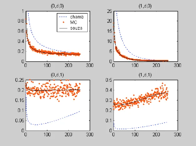
Figure 2 shows the spectral function derived in this paper for aggregated stock ARFIMA processes and the one derived in Chambers (1998), together with the periodogram ordinates averaged across 100 realizations of the process. The X axis shows the indices i = 1, 2, …, T/2 representing the Fourier frequencies i2π/T. Figure 3 does the same as Figure 2, but for flow processes. The processes are aggregated from ARFIMA(0,0.3,0), with n = 3; ARFIMA(1,0.3,0) with φ = 0.8 and n = 4; ARFIMA(0,0.3,1) with θ = -0.8 and n = 4; ARFIMA(1,0.3,1) with φ = -0.4, θ = -0.8 and n = 3. The aggregated series length is 512 observations and the error variance is taken as σε2 = 1.
Figure 2: Comparison between Chambers’s (1998) and this paper’s theoretical spectral
functions for aggregated stock ARFIMA processes, respectively the dashed and the continuous lines. The dots are the periodogram ordinates averaged across 100 realizations of the processes.
5 He did take it into account to derive the spectral function of a continuous ARFIMA process observed
As we can see for both stock and flow aggregated ARFIMA processes the averaged periodogram ordinates (dots) are scattered around the solid line, which represents the formula derived in this paper. The formula derived in Chambers (1998), represented by a dashed line, yields values somewhat different from the observed in the simulation experiment.
5 – Real example
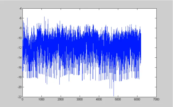
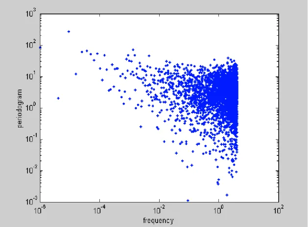
Chambers (1998) studies a number of UK macroeconomic flow series. He finds that the estimation using semiparametric methods is consistent with that the memory parameter remains unchanged after aggregation. The development of the theoretical results derived here suggests that his empirical results might be different if the variables were of the stock type. To verify the findings of the present paper, the daily US Dollar/ French Franc (US$/FF) exchange rate series is considered from October 20, 1977 to October 23, 2002 (25 years). More specifically, the natural logarithm of the squared returns is analysed. There are 68 (approximately 1.09%) zero returns existent in the 6264 workdays which were simply skipped, as well as the holidays. The series, its autocorrelation function (ACF) up to lag 1000 and its periodogram are shown in Figures 4-6, where the reader can notice the apparent long memory features such as persistently positive ACF (up to lag 250), and the periodogram scattered around a frequency power near the frequency zero.
return of exchange rates, the present analysis is consistent with the Long Memory Stochastic Volatility (LMSV) model of Breidt, Crato and Lima (1998), in which the returns are uncorrelated6 and are given by the following relation:
t t
t Y
R =σexp( /2)ε , (18)
where Yt is a stationary Gaussian long memory process independent of εt, mean zero
iid white noise. The analysed series is then:
t t t
t R Y v
Z ≡log( 2)=µ + + , (19)
where µ = (log σ2 + E[log εt2]) and vt = (log ε2 – E[log εt2]) is iid mean zero. Zt
is then a sum of a Gaussian long memory process and a white noise. The kurtosis of the series in study is approximately 3.68 and the skewness –0.79, so that the Jarque-Bera test rejects the hypothesis of Gaussianity at 1% confidence level. This does not mean that the Gaussianity of Yt is rejected since it is contaminated by the noise vt in
the observed Zt.
For the long memory study of the series, we shall utilize some semiparametric estimation methods. These are more adequate for the study than parametric methods, since it aims at the spectrum behaviour in the vicinity of the frequency zero as the arguments developed in Section 3.2 refer only to low frequency behaviour. The first method (GPH) was proposed by Geweke and Porter-Hudak (1983) and estimates d
using property (2). Taking the log of (2) on both sides,
j j f
j c d
I(λ )=log (λ)−2 [logλ ]+ε
log (20)
for frequencies near zero, where I(λj) is the periodogram. Defining j = 1, …, g(T), where g(T) = Tα and α∈ (0, 1), ordinary least squares regression on the set of Fourier frequencies λj gives the estimate of d. Hurvich, Deo and Brodsky (1998) provide the conditions which ensure the consistency of this estimator and Deo and Hurvich (2001) prove that the asymptotic distribution of this estimator for Zt is identical as for Yt provided a restriction in the bandwidth choice is observed.
The second method, denoted here by SMGPH, was proposed by Hassler (1993) and is similar to the GPH but uses a smoothed estimator for the spectrum
6
If one wants to allow the returns to exhibit serial correlation, one may relax the assumption that εt is
iid white noise in the model, but in this case the noise vt is not iid. For example, one may imagine that
(smoothed periodogram) instead of the raw periodogram. The third and last method, denoted by GSPR, is referred to as the Gaussian semi-parametric approach of Robinson (1995). This method is based on maximising the approximate form of the frequency domain Gaussian likelihood, where discrete averaging is carried out over a neighbourhood of zero frequency:
∑
∑
= =
−
= m
1 j
j m
1 j
j d 2
j log( )
m d 2 I m
1 log ) d (
R λ λ (21)
where m=Tα and α ∈ (0, 1). Robinson (1995) outlines the conditions under which the estimator is consistent.
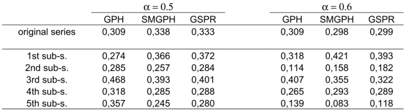
The series Zt displays long memory, as the modified R/S test of Lo (1991) rejects the hypothesis of short memory at a 0.5% level. Moreover, breaking up the series in five smaller sub-series of 1240 days7 yields estimates of the memory parameter consistent with the presence of long memory, as shown in Table 1.
Table 1: Estimates of the memory parameter with the three semiparametric estimators for the whole series Zt and for its sub-series, considering the bandwidth parameter α = 0.5 and 0.6.
α = 0.5 α = 0.6
GPH SMGPH GSPR GPH SMGPH GSPR original series 0,309 0,338 0,333 0,309 0,298 0,299
1st sub-s. 0,274 0,366 0,372 0,318 0,421 0,393 2nd sub-s. 0,285 0,257 0,284 0,114 0,158 0,182 3rd sub-s. 0,468 0,393 0,401 0,407 0,355 0,322 4th sub-s. 0,318 0,285 0,288 0,265 0,293 0,289 5th sub-s. 0,357 0,245 0,280 0,139 0,083 0,118
The series Zt is of stock type and is related to the instant volatility of the
returns, so that its aggregation would give a picture of this volatility measure once in a pre-determined period, say, a week. Note that this measure of volatility is not the usual squared returns8 but the log of it. Also, as proposed by Crato and Ray (2002), one might aggregate the series Zt as a flow variable so as to decrease the
signal-to-noise ratio with estimation purposes. Remember that Zt is a long memory process with
added noise. Table 2 compares the estimates for the original and the aggregated series
7
The five series correspond respectively to observations 1-1240; 1241-2480; 2481-3720; 3721-4960; and 4961-6196
8
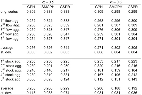
considering n = 5, with the aggregated time unit roughly corresponding to one week. There are n possible (different) aggregated series for each case (stock or flow), corresponding to the original series commencing at time t = 1, 2,…, n. All five are shown for each case and the same bandwidth choices as in Table 1, α = 0.5, 0.6. It is also shown their average and standard deviation across different commencing times in the original series.
Table 2: Estimates of the memory parameter with the three semiparametric estimators for the whole series Zt and for the aggregated flow and stock series, considering the bandwidth parameter α = 0.5 and 0.6.
α = 0.5 α = 0.6
GPH SMGPH GSPR GPH SMGPH GSPR orig. series 0,309 0,338 0,333 0,309 0,298 0,299
1st flow agg. 0,252 0,324 0,338 0,268 0,296 0,300 2nd flow agg. 0,260 0,325 0,339 0,281 0,307 0,309 3rd flow agg. 0,259 0,328 0,347 0,276 0,306 0,309 4th flow agg. 0,256 0,326 0,347 0,259 0,301 0,304 5th flow agg. 0,254 0,327 0,347 0,271 0,301 0,304
average 0,256 0,326 0,344 0,271 0,302 0,305 st. dev. 0,003 0,002 0,005 0,008 0,004 0,004
1st stock agg. 0,255 0,250 0,225 0,253 0,217 0,223 2nd stock agg. 0,280 0,201 0,250 0,320 0,216 0,216 3rd stock agg. 0,240 0,146 0,217 0,181 0,159 0,164 4th stock agg. 0,239 0,310 0,331 0,167 0,196 0,212 5th stock agg. 0,000 0,093 0,124 0,112 0,151 0,143
average 0,203 0,200 0,229 0,206 0,188 0,192 st. dev. 0,115 0,085 0,074 0,081 0,031 0,036
The example is very illustrative of a result proposed in this paper, namely that stock aggregates should be more biased in respect to long memory than flow aggregates, although the stock and flow aggregation of the same series may seem arbitrary. The clear picture of the result was made possible mainly because of the large amount of observations in the original series.
6 – Concluding Remarks
This paper derives the spectral density function of temporally aggregated long memory processes in light of the aliasing effect. The aggregation process is considered here the fact of observing the process at a slower sampling rate, giving rise to distinct interpretations: if the process is a stock variable, every n-th observation is considered, while if it is a flow variable, a sum of every n-th and their n-1 preceding observations is considered. Temporal aggregation is shown to maintain the integration order (the memory parameter d), with the exception of stock aggregates when d < 0 in the original series if the frequency-domain definition of d is considered (the integration order is always retained in the time-domain definition). A small Monte Carlo experiment is run, showing that the formulas for the spectral density function derived here match with the periodogram of synthetic series averaged across series, whereas some previous papers that addressed the subject do not provide accurate formulas.
From the spectral function of aggregated process derived here, I infer that flow aggregates from long memory processes shall have the estimates of d less biased than stock aggregates. This result is consistent with Souza and Smith (2002a, b) Monte Carlo results and is illustrated in Section 5 by an example with the daily US Dollar/ French Franc exchange rate series.
Acknowledgements
The author would like to thank FAPERJ for the financial support, EPGE for its kind hospitality and Marcelo Fernandes for helpful comments on previous versions of this work.
References
Andersen, T.G. and Bollerlev, T., “Answering the skeptics: yes, standard volatility models do provide accurate forecasts”, Int. Economic Review, 39, 885-905. Beran, J. (1994), Statistics for Long Memory Processes, Chapman & Hall.
Beran, J. and Ocker, D. (2000), “Temporal aggregation of stationary and nonstationary FARIMA(p,d,0) models”, working paper.
Bisaglia, L. & Guégan, D. (1998), “A comparison of techniques of estimation in long-memory processes”. Computational Statistics & Data Analysis, 27, 61-81. Booth, G.G., Kaen, F.R. and Koveos, P.E. (1982), “R/S analysis of foreign exchange
rates under two international monetary regimes”, Journal of Monetary Economics, 10, 407-15.
Breidt, F.J., Crato, N. and Lima, P. (1998), “The detection and estimation of long memory in stochastic volatility”, J. of Econometrics, 83, 325-348.
Brewer, K.R.W. (1973), "Some consequences of temporal aggregation and systematic sampling for ARMA and ARMAX models", J. of Econometrics, 1, 133-154. Chambers, M. J. (1998), “Long memory and aggregation in macroeconomic time
series”, Int. Economic Review, 39, 1053-1072.
Cheung, Y-W (1993), “Long memory in foreign exchange rates”, Journal of Business and Economic Statistics, 11, 93-101.
Crato, N. and Ray, B. K. (2002), “Semi-parametric smoothing estimators for long-memory processes with noise”, Journal of Statistical Planning and Inference, 105, 2, 283-97.
Deo, R. S. and Hurvich, C. M. (2001), “On the log periodogram regression estimator of the memory parameter in long memory stochastic volatility models”,
Econometric Theory, 17, 4, 686-710.
Diebold, F. X. and Rudebusch, G. D. (1989), "Long Memory and Persistence in Aggregate Output", Journal of Monetary Economics, 24, 189-209.
Granger, C. W. G. and Joyeux, R. (1980), “An introduction to long memory time series models and fractional differencing”. Journal of Time Series Analysis, 1, 15-29.
Geweke, J. & Porter-Hudak, S. (1983), “The estimation and application of long memory time series models”, Journal of Time Series Analysis, 4, 221-237. Hamilton, J. D. (1994), Time Series Analysis, Princeton Univ. Press, New Jersey. Hassler, U. (1993). “Regression of spectral estimators with fractionally integrated
Hosking, J. (1981), “Fractional differencing”. Biometrika, Vol. 68, No. 1, 165-176. Hotta, L. K. and Neto, J. C. (1993), "The effect of aggregation on prediction in
autoregressive integrated moving-average models", Journal of Time Series Analysis, 14, 261-269.
Hurvich, C. M., Deo, R. & Brodsky, J. (1998), “The mean square error of Geweke and Porter-Hudak’s estimator of the memory parameter of a long-memory time series”, Journal of Time Series Analysis, 19, 19-46.
Koopmans, L.H. (1974), The Spectral Analysis of Time Series, New York: Academic Press.
Lo, A.W. (1991), “Long-term memory in stock market prices”, Econometrica, 59, 5, 1279-1313.
Lütkepohl, H. (1986), “Comparison of predictors for temporally and contemporaneously aggregated time series”, International Journal of Forecasting, 2, 461-475.
Mandelbrot, B. B. (1965), “Une classe de processus stochastiques homothétiques à soi; application à la loi climatologique de H. E. Hurst”, Comptes Rendus Acad. Sci. Paris, 260, 3274-7.
Mandelbrot, B. B. and Van Ness, J. W. (1968), “Fractional Brownian motion, fractional noises and applications”, SIAM Review, 10, 422-437.
McLeod, A.I. and Hipel, K.W. (1978), “Preservation of the rescaled range I. A reassessment of the Hurst phenomenon”, Water Resources Research, 14, 491-508.
Oppenheim, A. V. and Schafer, R. W. (1989), Discrete-Time Signal Processing. New Jersey: Prentice-Hall
Otero, J. and Smith, J. (2000), “Testing for cointegration: power versus frequency of observation - further Monte Carlo results”, Economics Letters, 67, 1, 5-9. Priestley, M. B. (1981), Spectral Analysis and Time Series. London: Academic Press. Robinson, P. M. (1995). Gaussian semi-parametric estimation of long range
dependence. Annals of Statistics, 23, 5, 1630-1661.
Robinson, P. M. And Zaffaroni, P. (1998). “Nonlinear time series with long memory: a model for stochastic volatility”, Journal of Statistical Planning and
Inference, 68, 359-371.
Souza, L. R. and Smith, J. (2002b), “Temporal aggregation and fractional integration: a Monte Carlo study”, submitted to the International Journal of Forecasting. Teles, P. and Wei, W. W. S. (2002), “The use of aggregate time series in testing for
Gaussianity”, Journal of Time Series Analysis, 23, 1, 95-116.
Teles, P., Wei, W. W. S., and Crato, N. (1999), “The use of aggregate series in testing for long memory”, Bulletin of the International Statistical Institute, 52nd Session Book 3, 341-342.
Tschernig, R. (1995), “Long memory in foreign exchange rates revisited”, Journal of International Financial Markets, Institutions and Money, 5, 53-78.
Vilasuso, J. (2002), “Forecasting exchange rate volatility”, Econ. Letters, 76, 59-64. Wei, W. W. S. (1989), Time series analysis: univariate and multivariate methods,
Addison-Wesley.
Weiss, A. A. (1984), “Systematic sampling and temporal aggregation in time series models”, Journal of Econometrics, 26, 271-281.
Appendix
Proof of Theorem 1
The spectral density function of a covariance stationary discrete-time process Xt is
defined by:
∑
∞ −∞ = − = k jk x k x ef γ ω
π ω
2 1 )
( , -π < ω ≤ π (A1)
where γkx is the k-th order autocovariance of Xt. As the autocovariance function of
real valued processes is an even function, (A1) reduces to:
∑
∞ −∞ = = k x k x kf γ ω
π
ω cos
2 1 )
( , -π < ω ≤ π (A2)
fx(ω) is then defined as a Fourier cosine series whose coefficients are the
autocovariances of Xt. As cos kω, k = 0, 1, 2, ..., is a complete orthogonal set over the
interval (–π, π] for even functions (and the spectral density is an even function) the relation given by (A2) is equivalent to:
,... 2 , 1 , 0 ), ( cos cos ) ( = = ± ± =
∫
∫
− − k ω dF k dω kfx x
x k π π π π ω ω ω γ (A3)
where Fx(ω) is the spectral distribution function of Xt. The autocovariances of Yt =
Xnt are given thus by:
,... 2 , 1 , 0 ), ( cos cos ) ( = = ± ± = =
∫
∫
− − k ω dF nk dω nkfx x
x nk y k π π π π ω ω ω γ γ (A4)
First take the simpler case where n is an odd number. The integral in (A4) can be split into:
∑ ∫
∑
∫
− − − = − − − − = + − + + = = = 2 1 2 1 / / 2 1 2 1 / ) 1 2 ( / ) 1 2 ( ) / 2 ( ) 2 cos( ) ( cos n n i n n x n n i n i n i x y k n i ω dF ik nk ω dF nk π π π π π π ω ω γ (A5)Since cos(a + 2iπ) = cos(a), where i is an integer number, (A5) rewrites to:
∑ ∫
− − − = − + = 2 1 2 1 / / ) / 2 ( ) cos( n n i n n x yk nk dF ω i n
π
π
π ω
γ (A6)
Making λ= nωwhere λ is the frequency measured in the same time unit as Yt, we can
∑ ∫
− − − = − + = 2 1 2 1 ) / 2 / ( 1 ) cos( n n i x yk dF n i n
n k π π π λ λ γ (A7)
However, by (A3) we can write the k-th order autovariance of Yt as:
,... 2 , 1 , 0 ), ( cos cos ) ( = = ± ± =
∫
∫
− − k dF k d kfy y
y k π π π π λ λ λ λ λ γ (A8)
The fact that cos kλ, k = 0, 1, 2, ..., is a complete orthogonal set over the interval (–
π, π] for even functions, together with (A7) and (A8) imply (6). Now if n is an even number (A5) rewrites to:
∑ ∫
∑ ∫
− − = − = − + + + + + + = 1 2 2 / 0 2 2 1 0 / ) / 2 ( ) 2 cos( ) / 2 ( ) 2 cos( n n i n x n n i n x y k n i ω dF ik nk n i ω dF ik nk π π π π ω π π ω γ (A9)and the rest of the proof follows as in the case n is odd.
Proof of Theorem 2
Let
∑
− = = 1 0 n i t it B X
Z be the overlapping aggregated process of Xt. The moving average
representation of (1 + B + … + Bn-1) straightforwardly gives the following relationship between the spectra of Zt and Xt:
2 1 0 ) ( ) (
∑
− = − = n k jk xz f e
f λ λ λ , -π < λ ≤ π (A10)
The quantity 2 1 0
∑
− = − n k jke λ rewrites as:
= + = − =
∑
∑
∑
∑
− = − = − = − = − 2 1 0 2 1 0 2 1 0 2 1 0 sin cos sin cos n k n k n k n k jk k k k j ke λ λ λ λ λ
(
)
∑ ∑
(
)
∑
− = − + = − = + + + = 1 0 1 1 1 0 2 2 sin sin cos cos 2 sin cos n k n k i n k iλ kλ i k kkλ λ λ λ (A11)
∑
∑ ∑
∑
− − = − = − + = − =− = + − = 1 −
1 1 0 1 1 2 1 0 cos ) ( ] ) cos[( 2 n n k n k n k i n k jk k k n k i n
e λ λ λ (A12)
Using equation (6.1.43) of Priestley (1981, p. 400), which is based on further trigonometric manipulation, in (A12) and correcting for the case λ = 0, gives
) ( . 2 ) 2 / ( ) 2 / ( lim 2 2 2 1 0 λ π θ θ λ θ λ n n k jk F n sin n sin
e = =
→ −
= −
∑
, (A13)where Fn(λ) is the Fejer kernel. Equations (A10) and (A13) imply equation (8) and the proof is complete.
Proof of Proposition 1
The proof of 1a) is straightforward since Assumption 1 assures that Xt is covariance
stationary and hence
∑
∞ = ∞ < 0 2 i ia . Requiring the covariance stationarity of Xt in
Assumption 1 is necessary because if, for example, (1-B)d* Xt = εt, where 1 > d* >
0.5, the representation d t
i i t i t d B w X
B ε */2ε
0 2 / * ) 1 ( ) 1 ( − ∞ = − − = =
−
∑
would satisfy theWold representation in (11) but
∑
∞=0 2
i i
a would diverge.
Proof of 1b): By the Definition 3b)
∑
== n
i
nt i
t B X
Y 1
. Let
∑
== n
i
t i
t B X
Z 1
so that Yt = Znt.
Since
∑
∞ = − = 0 i i t i t aX ε then
∑
∑
∑
∞ = − ∞ = − − = = = 0 0 1 0 i i t i i i t i n k k
t B a b
Z ε ε , where
∑
+ − = = i n i k k i a b 1
and ak
= 0 for k < 0. It remains to prove that
∑
<∞ ∞=0 2
i i
b and then the proof of 1b) is similar the proof of 1a). This condition is equivalent to say that the variance of Zt is finite.
Since Xt has finite variance, VAR(Zt) ≤ n2 VAR(Xt) and is finite. The proof is
complete.
Proof of Lemma 1
summations have n different terms. Suppose n is even. For example, e-j(λ−(n/2)2π)/n is indistinguishable from e-j(λ+(n/2)2π)/n , that is, the results for i = -n/2 and i = n/2 are the same.
2b) The proof of 2b follows directly from Corollary 1, using the same change in the summation indices as in 2a.
Proof of Proposition 2
2a) If Xt is a stock variable, the autocorrelations of the aggregated process behave like
1 2 1 2 ) ( ) )( ( ~ − = − = d y d x x nk y
k ρ cρ nk nk cρ k k
ρ as k tends to infinity, which satisfies (1). If Xt is a flow variable, we only need to prove that the overlapping aggregated
variable
∑
== n
i
t i
t B X
Z 1
satisfies (1). Hence, using the fact that Yt = Znt, the remaining
of the proof is identical to the proof for a stock variable. By equation (1), γkx ~ σx2 cρ(k)k2d-1 as k →∞. For the sake of simplicity assume E[Xt] = 0. So, γkx =E
[
XtXt+k]
.The autocovariances of Zt (k≥0) are given then by
[
]
xi k n n i n i i k t n i i t k t t z k z
k E Z Z E X X n i +
− + − = − = + − − = − + −
∑
∑
=∑
− = ==γ γ
γ 1 1 1 0 1 0 |) |
( . (A14)
Take the Taylor series expansion of (k+i)2d-1 around k2d-1:
(k+i)2d-1 = k2d-1 + i.(2d-1) k2d-2 + (i2/2)(2d-1)(2d-2) k2d-3 + O(k2d-4). (A15)
If the right hand side of equation (A14), substituting (1) for γk+ix, is expanded in Taylor series of this type (A15), the series second terms cancel out in the summation and hence γkz ~ n2σx2cρ(k)k2d-1+ O(k2d-3) as k →∞, and consequently ρkz ~ cρz(k)k2d-1. The proof of 2a is complete.
2b) If Xt is a covariance stationary stock variable and λ ≥ 0, Theorem 1 says that
( )
∑
− − = + = =− 1/2
2 / ) / ] 2 ([ 1 ) ( ) ( n n i x y
y f i n
n f
f λ λ λ π , where . is the integer operator. As
fx(i2π/n), i ≠ 0, is finite and has finite neighbourhood, and Xt satisfies Definition (2),
the term in the summation corresponding to i = 0 dominates the others as λ→ 0. The spectral function of Yt thus satisfies:
Now if Xt is a flow variable, then
[
]
( )
∑
−− =
+ +
= 1/2
2 /
) / ] 2 ([ ). / ] 2 ([ 2
) (
n
n i
n x
y f i n F i n
f λ π λ π λ π
as stated in Corollary 1. The Fejer kernel Fn(.) and its first derivative are zero valued in the nonzero multiples of the Nyquist frequency 2π/n and hence the term
corresponding to i = 0 in the summation dominates the others however value d takes. Furthermore Fn(0) = n/2π so that the spectrum of Yt behaves like: fy(λ) ~ n.fx(λ/n) ~ n2d+1.cfx(λ/n) |λ|-2d as λ→ 0, satisfying (2) with the same integration order d. The proof of 2b is complete.
2c) The proof that condition (2) with a negative memory parameter d still holds after flow aggregation is given in the proof of 2b. It does not apply for stock aggregation because if d < 0, the term corresponding to i = 0 in the summation in (16) is
dominated by the other positive terms, as limλ→0 |λ|-2d = 0 and condition (2) is thus
violated. The proof of 2c is complete.
Proof of Proposition 3
Suppose (1) and (2) hold for a stock variable Xt with d < 0, for example Xt might be
an ARFIMA(0,d,0), d < 0. Take the aggregated variable Yt. By Proposition 2a
condition (1) still holds for Yt while by 2c condition (2) does not hold for Yt. Hence
Figure 4: US$/FF exchange rate, logarithm of the squared returns from October 20, 1977 to October 23, 2002. The series.
![Figure 1: The Fejer kernel for n = 6, restricted to (- π , π ]](https://thumb-eu.123doks.com/thumbv2/123dok_br/15628490.109029/10.892.134.726.203.522/figure-fejer-kernel-n-restricted-π-π.webp)