On Superstatistical Multiplicative-Noise Processes
S´ılvio M. Duarte Queir´os∗
Centro Brasileiro de Pesquisas F´ısicas, Rua Dr. Xavier Sigaud, 150, 22250-250 Rio de Janeiro - RJ, Brazil
Received on 28 September, 2007
In this article we analyse the long-term probability density function of non-stationary dynamical processes with time varying multiplicative noise exponents which are enclosed inwards the Feller class of processes. The update in the value of the exponent occurs in the same conditions as presented by BECKand COHENfor superstatistics. Moreover, we are able to provide a dynamical scenario for the emergence of a generalisation of the Weibull distribution previously introduced.
Keywords: Multiplicative noise; Superstatistics; Generalized Weibull distribution
I. INTRODUCTION
The description within a physical context of driven non-equilibrium complex systems has frequently been made by considering that their dynamical behaviour is characterised by spatial-temporal fluctuations of some parameter, ˜β. Usually, this parameter has been considered to be the (inverse) temper-ature, the dissipation of energy in turbulent flows, the ampli-tude of Gaussian white noise, thelocalmean-reverting value or thelocalvariance. As an example, we mention the stan-dard case of a Brownian particle diffusing along an inhomo-geneous medium in which temperature (hence diffusion “con-stant”) fluctuates in both space and time. In this approach, as it can be understood, there are two important time scales: the scale in which the dynamics is able to reach a stationary state (assuming a fixed value for parameter ˜β), and the scale at which the fluctuating parameter evolves. A particular case to consider is when these two time scales are clearly separated, specifically, when the time needed for the system to reach sta-tionarity (considering a predetermined ˜β) is much smaller than the scale at which that parameter changes. In the long-term, the non-equilibrium system is described by the superposition of different local dynamics at different time intervals that was coined by BECKand COHENassuperstatisticsor “statistics of statistics” [1, 2]. Frequently, systems that are characterised as “superstatistical” exhibit non-Gaussian distributions with kur-tosis excess, or distributions with non-exponential decay. In addition, superstatistical systems present a parameter, ˜β, that fluctuates on a large scale,T, and follows a time-independent distribution, p(β˜). The superstatistical framework has suc-cessfully been applied on a widespread of problems like: in-teractions between hadrons from cosmic rays [4], fluid tur-bulence [3, 5, 6], granular material [7], electronics [8], eco-nomics [9–12], among many others [13]. Furthermore, it has been regarded as a possible foundation for non-extensive sta-tistical mechanics [3] based on Tsallis entropy [14] as we show later on. In this manuscript we introduce a different analysis of differential stochastic dynamics in which the
ex-∗Present address: Unilever R & D, Port Sunlight, Quarry Road East ,
Be-bington, Wirral CH63 3JW, United Kingdom; Electronic address:sdqueiro@ cbpf.br,[email protected]
ponent of a Feller process is assumed as the superstatistical parameter. The main advantage of this proposal is that it per-mits the evolution of the functional form of the second-order Kramers-Moyal moment in opposition to previous presenta-tions.
II. SUPERSTATISTICS
Consider an inhomogeneous system composed by a large set of cells that have different values of some parameter ˜βas we have referred to here above. Within each cell, local equi-librium is reached very promptly. The parameter ˜βis taken as constant throughout a period of timeT after which it changes into a new value. This update occurs always in accordance with a distribution p(β˜)for the parameter. Taking into con-sideration that each cell is in local equilibrium, thus present-ing a Boltzmann factor,e−βE,1the long-term stationary dis-tribution2of the non-equilibrium system is obtained from a weighted average oflocalBoltzmann factors, withβ≡β³β˜´,
P(E) = Z
p³β˜´ρ(E)e−
βE
Z(β)dβ˜, (1)
whereρ(E)represents the density of states, andZ(β)the nor-malisation constant. Going back to the example of a Brown-ian particle moving across a medium treated in Ref. [3], we get that its velocity,~v, is obtained from the local Langevin equation,
d~v=−γ~v dt+σdW~t. (2) Seeing that the medium is inhomogeneous, eitherγ[15] orσ vary from cell to cell on a large time scaleT 3. Therefore, local Boltzmann factor has,
β= 2γ
mσ2, (3)
1Eis the effective energy in each cell. 2The observation timet≫T.
3Ifγis the random parameter then, ˜β=γ, else ifσis the random parameter
which is random. From Eq. (3), the parameterβ can also fluctuate for the case of a particle with varying mass [16].
Within time scale T, and according to Eq. (2), the local stationary distribution of velocities is a Gaussian conditioned to valueβ,
p′(~v|β) =
µ β
2π ¶d/2
exp ·
−1 2βm~v
2 ¸
. (4)
If the system is able to reach some local equilibrium before an update of ˜βtakes place, i.e.,T ≫γ−1=τ, then, we can determine the marginal velocities probability distribution of the long-term behaviour of the Brownian particle,
P(~v) =
Z ∞
0
p(β)p′(~v|β)dβ. (5) Hence, it is straightforward to verify that the form of P(~v)
depends explicitly on the functional form of p(β). Specif-ically, it was verified in Ref. [3] that, when p(β) is the χ2−distribution withndegrees of freedom, Eq. (5) yields,
P(~v) = 1
Z £
1+ (1−q)β0~v2 ¤1/(1−q)
, (6)
whereq=1+ 2
n+d,Z is the normalisation factor, andβ0the average inverse temperature (see Ref. [1] for details). Such a distributionP(~v)maximises Tsallis entropy [14],
Sq=1− R
[p(x)]qdx
q−1 (q∈ℜ). (7)
This fact has turned out superstatistics into the first dynami-cal scenario for the emergence of non-extensive statistidynami-cal me-chanics [17].
III. THE MODEL
Consider the following one-dimensional stochastic differ-ential equation,
dv=−γv dt+ω£
v2¤αdWt, (v6=0 if α<0), (8) whereWt is a regular Wiener stochastic process,i.e.,hdWti= 0, and hdWtdWt′i = dtδ(t−t′) 4. Stochastic equation (8) belongs to the Feller class of (multiplicative noise) processes [18] withγ≥0,α<1
4 for a (time-dependent) nor-malisable probability density function (PDF) f(v,t). The as-sociated Fokker-Plank Equation of Eq. (8) is
∂f(v,t)
∂t = ∂
∂v[γv f(v,t)] + 1 2
∂2 ∂v2
h ω2£
v2¤2α f(v,t)i, (9)
4The main advantage of writing£
v2¤α
instead of|v|α′withα′=2αis that
of analyticity for allvwhenα>0.
whose solution f(v,t)relaxes exponentially with a character-istic time,τ, into the stationary solution,
p(v) = 1
Zexp ·
− γ
ω2(1−2α)v
2(1−2α)¸¡
v2¢−2α, (10)
i.e., a Weibull-like distribution,
W
(v).Zis the normalisation constant,Rp(v) dv,
Z= 2
1−4α
· γ
ω2(1−2α) ¸14−α−4α2
Γ ·
2+ 1
4α−2 ¸
. (11)
Forα=0, Eq. (8) becomes the standard Langevin equation, andp(v)the Gaussian distribution,
G
(v) = 1Zexp h
−ωγ2v2i, (12)
withZ=qπ ωγ2.
After the transient, f(v,t)≈p(v). The mean value of v, ¯
v≡R
v p(v)dv, is equal to zero as well as all odd moments of p(v). Regarding the second-order moment,v2≡R
v2p(v)dv, we have got
v2= ω2
2γ if α=0
4α−1 4α−3
hω2(1−2α) γ
i1−12α Γ[5−8α
2−4α] Γ[2+ 1
4α−2]
if α6=0
. (13)
If we considervas the velocity of a particle of unitary mass which does a 1D random walk, using equipartition theo-rem we are able to determine the inverse temperature, β≡
(k T)−1 5, yielding
β=v2. (14)
Evaluating the kurtosis
κ≡³v2´−2
Z
v4p(v)dv, (15) we have obtained
κ=
3 if α=0
(3−4α)2 (4α−5)(4α−1)
Γ[7−8α
2−4α]Γ[2+4α1−2]
{Γ[5−8α 2−4α]}
2 if α6=0
. (16)
As it is visible from Fig. 1, distribution (10) is platykurtic for α<0, and leptokurtic forα>0.
Moving on, we shall now consider thatexponentαinstead of constant, varies according to superstatistical requirements. In other words, let us consider an inhomogeneous system which is composed by a large set of cells that have differ-ent values ofα. Within each cell, the value ofαis updated at
-4 -3 -2 -1 0 1
1.5 2 2.5 3
-5
k
a
0.05 0.1 0.15 0.2 0.25
5 10 50 100 500 1000
0 1
a
k
FIG. 1: Kurtosis,κ, vs. α. Upper panel: Non-positive values of
α which lead into platykurtic distributions. In the limitα→ −∞,
κ=1. Lower panel: Non-negative values ofαleading into leptokur-tic distributions which hasα= 14 as upper bound. The dashed line corresponds to the kurtosis of a Gaussianκ=3.
every elapsed time intervalℓ, in agreement with a certain PDF ρ(α). The update scale, ℓ, is much greater than relaxation time scale τ. Noticing that each cell is in local equilibrium, the long-term stationary distribution of the non-equilibrium system is obtained performing the integral,
P(v) = Z
ρ(α)p(v)dα. (17) As possible applications of such a model we name: descrip-tion of velocities in granular material (particularly see figures of Ref. [19]) and unconventional turbulent fluids, or even the dynamics of financial observables. Explicitly, systems which undergo through different phases during their time evolution or situations where different stages are measured when obser-vations are made at the same point of space. In a thermody-namic context, the fluctuations inαcorrespond to fluctuations in temperature, but obtained through a completely different way from the proposal presented in Ref. [3]. Specifically, fluc-tuations inαinduce a modification of the functional form of the 2ndorder Kramers-Moyal coefficient, while in Ref. [3] its functional form is always preserved.
A. Some examples
1. Dichotomous case
This case represents the simplest form to introduce fluctua-tions inα, and for which a full analytical treatment is possible.
Its probability density function is simply,
ρ(α) =1
2δ(α−α0) + 1
2δ(α−α1), (α06=α1). (18)
Amongst all endless possibilities forα0andα1, let us firstly consider cases for which one of the exponents is equal to zero. The long-term distribution is thus given by
P(v) =1
2
G
(x) + 12
W
α(x). (19)For small values of|v|, andα<0,P(v)approaches the limit q γ
4π ω2 as
£ v2¤−2α.
In Fig. 2 we exhibit the resulting probability density func-tion,P(v), forα0=0, andα1=−1, α1=−12, andα=15. The valuev2
e f,
v2e f ≡
Z
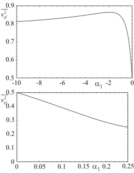
v2P(v)dv, (20) is presented in Fig. 3 for several values ofα1.
-3 -2 -1 0 1 2 3 4
0.1 0.2 0.3 0.4 0.5
-4 0 0.6
P( )v
v
0.1 0.2 0.5 1 2 5 10
10 -13 10 10
-10 -7 10 -4
P( )v
10 -1
10 -16
v
FIG. 2: Probability density functionP(v)vs. vfor the case of su-perstatistical processes with a dichotomous distribution (18) where
γ=ω=1. Upper panel: In both casesα0=0, andα1=−1 for the full line, andα1=−12for the dashed line. Lower panel:P(v)vs.v for a dichotomous case withα0=0 andα=15 (γ=ω=1) in a log-log scale. For this case, the variancev2
e f =0.2860. . .and kurtosis
κ=11.953. . ..
2. Uniform distribution case
-8 -6 -4 -2 0 0.6
0.7 0.8 0.9
-10 0.5
a
1vef 2
0.05 0.1 0.15 0.2 0.25
0.1 0.2 0.3 0.4 0.5
0 0 vef
2
a
1FIG. 3: Standard deviation,v2e f,vs. dynamical exponentα1for su-perstatistical process with a dichotomous PDF (18) whereα0=0, andγ=ω=1. Forα1=0,v2e f =
1
2, and forα1=−∞the value ofv2e f tends to 34 (upper panel). For positive values ofα1,v2e f is a
monotonically decreasing function ofα1withv2e f=
1
4forα1= 14.
evolves according to a uniform distribution betweenα0eα1,
ρ(α) =
1
α0−α1 if α1≤α≤α0
0 otherwise
. (21)
However, it is possible to evaluate numerically the form of the long-term distribution as we present for two particular cases in Fig. 4. Computing the kurtosis,κ, for both cases we have verified that the two examples are platykurtic.
Another possibility is to consider just non-negative values forα. This situation is more likely to be experimentally veri-fied, since kurtosis excess is quite ubiquitous. In this case, and since we are considering leptokurtic distributions,P(v)is also leptokurtic. An illustration of this sort of example is presented in Fig. 5 whereαuniformly varies between 0 and 15.
Moreover, extending our range of values for exponent α, we can consider positive and negative values as we present in Fig. 6. For this last case, in the long-term, the system endures both platykurtic and leptokurtic regimes.
3. Theχ2-distribution
Another distribution that appears in various phenomena is theχ2-distribution,
ρ(α) = ν
ν
¯ α Γ[ν]
µ |α|
¯ α
¶ν−1
exph−ν ¯ α|α|
i
. (22)
FIG. 4: Numerically obtained probability density functionP(v)vs. vfor the case of superstatistical processes with uniform distribution, Eq. (21) whereγ=ω=1. The black line corresponds toα0=0, and
α1=−12, withv2e f =0.833. . ., and kurtosis,κ=1.755. . .. The grey line corresponds to a uniform distribution withα0=−12 α1=−32
yieldingv2e f=1.169. . ., and kurtosis,κ=1.179. . ..
For this case an analytical form is not, in principle, possible to obtain. Nonetheless, we obtain the numerical solution for P(v)as we show in Fig. 7.
B. A generalised Weibull distribution
In this subsection we treat, the standard case where in Eq. (8)ωevolves on a superstatistical fashion rather thanα. For this particular case, whenΩ≡ω−2follows aχ2-distribution,
ρ(Ω) = 1
Ω0Γ£ν2¤ µ ν
2Ω0 ¶ν2
Ω2+ν2exp·−ν
2 Ω Ω0
¸
, (23)
the long-term stationary distribution,P(v), that corresponds to a weighted average of p(v)over all possible values ofΩ, yields
q
W
(v) = 1 Z′expq" −
¡ v2¢a
˜ v
# ¡
v2¢b, (24)
where,
q=4+ν−6α−2ν α
2+ν−2α−2ν α, v˜=
ν(1−2α)2Ω0
(2+ν−2α(1+ν))γ, (25)
and
FIG. 5: Left panel: The full line represents the numerically obtained probability density functionP(v)vs. vfor the case of superstatistical processes with uniform distribution, Eq. (21), whereα0=0, andα1= 15(γ=100,ω=10). The dashed line represents the PDF of the upper boundα=15, and the dotted line the PDF of the lower boundα=0 (a Gaussian). The long-term PDF decays slower than the Gaussian. The grey symbols represent the PDF obtained from the numerical simulation of a superstatistical system with the same parametersγandωand PDFρ(α). In the inset we showρ(α)of that process. Right panels: Excerpt of a superstatistical time series ofvwhich evolves according to Eq. (8) withγ=100,ω=10, andαassociated with a uniform distribution betweenα=0 andα= 15. The time scale of updatingαis 1 time unit which is rather larger than 10−2that is the time scale of relaxation towards stationarity. For this caseα
0=0, andα1= 15, with v2e f=0.285. . ., and kurtosis,κ=5.272. . .. A fair similar distribution, namely Fig. 6(b), has been obtained in Ref. [20] for the velocities PDF of a long-range Hamiltonian system at a quasi-stationary state.
FIG. 6: Numerically obtained probability density functionP(v)vs. vfor the case of superstatistical process with uniform distribution, Eq. (21), whereα0=−15, andα1= 15 (γ=ω=1). In this case v2
e f =0.476. . ., and kurtosis,κ=3.129. . .. Interestingly, this ex-ample suggests the existence of, at least, one distributionρ(α)with
α06=α16=0 for whichP(v)is mesokurtic.
Eq. (24) goes to zero as a power law with exponentb, and for large|v|, the same distribution also vanishes as a power law but with exponent a/(1−q) +b. For this case, it is possi-ble to evaluate even moments of ordermwhen the following conditions are verified,
a>0, b>−m+1 2 ,
a
q−1−b> m+1
2 . (27)
Whenb=0,i.e.,α=0,P(v)turns into aq-Gaussian distrib-ution recovering the scenario of Ref. [3]. In Fig. 8 we depict
FIG. 7: Numerically obtained probability density functionP(v)vs. vfor the case of superstatistical processes with aχ2-distribution, Eq. (22) whereν=5, andα=γ=ω=1. For this example we have v2e f=1.150. . ., and kurtosis,κ=1.999.
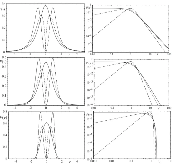
examples ofq
W
(v)for some values ofa,b, andq.IV. REMARKS AND PERSPECTIVES
-4 -2 0 2 4 0.1
0.2 0.3 0.4
0 P( )v
v 10 -60.01 0.1 1 10 100 10
10 10 10 1
-5 -4 10 -3 -2 -1
P( )v
v
-4 -2 0 2 4
0.1 0.2 0.3 0.4 0.5
0
P( )v
v 10 -60.01 0.1 1 10 100
10 10 10 10 1
-5 -4 10 -3 -2 -1 P( )v
v
-4 -2 0 2 4
0.2 0.4 0.6 0.8
0
P( )v
v 10 -60.001 0.01 0.1 1 10
10 10 10 10 1
-5 -4 10 -3 -2 -1
P( )v
v
FIG. 8: Representation ofqW(v)vs. vfor several values of parametersa,b,q, and ˜v=1. Left panels contain linear-linear representations,
whereas right panels exhibit the sameqW(v)but in a log-log scale. For long dashed lines(a=2,b=1); short dashed lines
³
a=5 4,b=
1 4
´
;
and for the full lines(a=1,b=0)which correspond to aq-Gaussian PDF. In upper panels we haveq=74. Because of conditions (27), the
(a=2,b=1)case is the only one to have a finitev2e f . Explicitly,v2e f=6.424. . .. Midst panels:q= 3
2. Both of the three cases have a finite v2e f. Specifically,v2e f =√2 for(a=2,b=1),ve f2 =2 for(a=1,b=0), andv2e f =24/5for
³
a=54,b=14´. Curiously, case(a=2,b=1)
hasκ=3 just like a Gaussian distribution,i.e., a mesokurtic distribution. Lower panels: q=3
4. In this case, distributions present a compact
support,[−vc,vc], by reason of Tsallis cut-off, wherevc=
³
1 1−q
´21a
.
one that is equivalent to the evolution of the noise width in the stochastic term of the corresponding differential equation. The main advantage of the former is the possibility of mim-icking systems which hold a rather complex dynamics that goes through a (random) sequence of dynamical regimes. We have determined either analytically or numerically the long-term probability density function which can assume all types of kurtosis. Concerning the latter superstatistical approach, we have verified that it allows the emergence of a generalisa-tion of the Weibull distribugeneralisa-tion within the framework of Tsal-lis non-additive entropy. This distribution has proved to be valid for numerical adjustments in a large variety of systems. For theq-Weibull, we have also been able to obtain platykur-tic, mesokurplatykur-tic, and leptokurtic distributions. In respect of is actual implementation to the analysis of experimental data
we must refer that it requires the development of techniques to capture both ofρ(α)andT as it was introduced for cases with fluctuations inω[5][24]. The solution for this non-trivial challenge either on an experimental or theoretical level is cer-tainly welcomed.
Acknowledgments
I am deeply grateful to Professor Constantino Tsallis who has always stimulated my scientific curiosity with his observa-tions, comments, and endless incentive. I thank D. O. Soares-Pinto for calling my attention to the work of Ref. [19], and to E.M.F Curado and F.D. Nobre for their ever useful comments. This work benefited from financial support from Fundac¸˜ao para a Ciˆencia e Tecnologia (Portuguese Agency), and also in-frastructural support from PRONEX (Brazilian agency). The present piece of work pays homage to Brasil and its
flamboy-ant people where and with whom I have had the best times of my life.
Note after acceptance- During a talk given in November 2007 at Queen Mary University of London based on this work I took knowledge by Prof. C. Beck of an article on turbu-lence, namely, Ref. [25], in which are presented probability density functions with an aspect very similar to some of the distributions presented herein. This underlines the surmised application of the our theoretical model to turbulence models.
[1] C. Beck and E. G. D. Cohen, Physica A322, 267 (2003). [2] S. Abe, C. Beck, and E.G.D. Cohen, Phys. Rev. E76, 031102
(2007).
[3] C. Beck, Phys. Rev. Lett.87, 180601 (2001).
[4] G. Wilk, Z. Włodarczyk, Phys. Rev. Lett.84, 2770 (2000). [5] C. Beck, E. G. D Cohen, and H.L. Swinney, Phys. Rev. E72,
056133 (2005).
[6] S. Rizzo and A. Rapisarda,Proceedings of the 8th Experimental Chaos Conference, Florence, AIP Conf. Proc. No. 742 (AIP, Melville 200), 176; C. Beck, E. G. D. Cohen, and S. Rizzo, Europhys. News36, (6) 189 (2005); C. Beck, Phys. Rev. Lett.
98, 064502 (2007).
[7] C. Beck, Physica A365, 96 (2006).
[8] F. Sattin and L. Salasnich, Phys. Rev. E65, (R)035106 (2002). [9] J.P. Bouchaud and M. Potters,Theory of Financial Risks: From Statistical Physics to Risk Management, (Cambridge University Press, Cambridge, 2000); M. Ausloos and K. Ivanova, Phys. Rev. E68, 046122 (2003).
[10] S. M. Duarte Queir´os and C. Tsallis, 2005 Europhys. Lett.69, 893 (2005); S. M. Duarte Queir´os, Physica A344, 619 (2004); S. M. Duarte Queir´os and C. Tsallis, 2005 Eur. Phys. J. B48, 139 (2005).
[11] S. M. Duarte Queir´os, Europhys. Lett.71, 339 (2005). [12] J. de Souza, L. G. Moyano, and S.M. Duarte Queir ´os, Eur. Phys.
J. B50, 165 (2006).
[13] C. Beck, Europhys. Lett.64, 151 (2003); A. M. Reynolds, Phys.
Rev. Lett.91, 084503 (2003); N. Mordant, A. M. Crawford, and E. Bodenschatz, Physica D193, 245 (2004); S. Jung and H. L. Swinney, Phys. Rev. E72, 026304 (2005); C. Beck, Physica D193, 195 (2004); K. E. Daniels, C. Beck, and E. Boden-schatz, Physica D193, 208 (2004); C. Beck, Physica A331, 173 (2004); S. Abe and S. Thurner, Phys. Rev. E72, 036102 (2005).
[14] C. Tsallis, J. Stat. Phys.52, 479 (1988).
[15] J. Łuczka, P. Talkner, and P. H¨anggi, Physica A278, 18 (2000). [16] M. Ausloos and R. Lambiotte, Phys. Rev. E73, 011105 (2006). [17] E. G. D. Cohen, Pramana, J. Phys.64, 635 (2005).
[18] W. Feller, Ann. Math.54, 173 (1951).
[19] W. A. M. Morgado and E. R. Mucciolo, Physica A311, 150 (2002).
[20] A. Pluchino, A. Rapisarda, and C. Tsallis, EPL 80, 26002 (2007).
[21] S. Picoli Jr., R. S. Mendes, and L. C. Malacarne, Physica A324, 678 (2003).
[22] I. W. Burr, Ann. Math. Stat.13, 215 (1942); S. Nadarajah and S. Kotz, Physica A377, 465 (2007).
[23] G. A. Tsekouras and C. Tsallis, Phys. Rev. E71, 046144 (2005). [24] S. M. Duarte Queir´os, Physica A385, 191 (2007).