HESSD
8, 8203–8229, 2011Analysis of parameter uncertainty in
hydrological
Z. Y. Shen et al.
Title Page
Abstract Introduction
Conclusions References
Tables Figures
◭ ◮
◭ ◮
Back Close
Full Screen / Esc
Printer-friendly Version Interactive Discussion
Discussion
P
a
per
|
Dis
cussion
P
a
per
|
Discussion
P
a
per
|
Discussio
n
P
a
per
|
Hydrol. Earth Syst. Sci. Discuss., 8, 8203–8229, 2011 www.hydrol-earth-syst-sci-discuss.net/8/8203/2011/ doi:10.5194/hessd-8-8203-2011
© Author(s) 2011. CC Attribution 3.0 License.
Hydrology and Earth System Sciences Discussions
This discussion paper is/has been under review for the journal Hydrology and Earth System Sciences (HESS). Please refer to the corresponding final paper in HESS if available.
Analysis of parameter uncertainty in
hydrological modeling using GLUE
method: a case study of SWAT model
applied to Three Gorges Reservoir
Region, China
Z. Y. Shen1, L. Chen1, and T. Chen1
1
State Key Laboratory of Water Environment Simulation, School of Environment, Beijing Normal University, Beijing 100875, China
Received: 17 August 2011 – Accepted: 19 August 2011 – Published: 31 August 2011
Correspondence to: Z. Y. Shen ([email protected])
HESSD
8, 8203–8229, 2011Analysis of parameter uncertainty in
hydrological
Z. Y. Shen et al.
Title Page
Abstract Introduction
Conclusions References
Tables Figures
◭ ◮
◭ ◮
Back Close
Full Screen / Esc
Printer-friendly Version Interactive Discussion
Discussion
P
a
per
|
Dis
cussion
P
a
per
|
Discussion
P
a
per
|
Discussio
n
P
a
per
Abstract
The calibration of hydrologic models is a worldwide difficulty due to the uncertainty involved in the large number of parameters. The difficulty even increases in the re-gion with high seasonal variation of precipitation, where the results exhibit high het-eroscedasticity and autocorrelation. In this study, the Generalized Likelihood
Uncer-5
tainty Estimation (GLUE) method was combined with Soil and Water Assessment Tool (SWAT) to quantify the parameter uncertainty of the stream flow and sediment simu-lation in the Daning River Watershed of the Three Gorges Reservoir Region (TGRA), China. Based on this study, only a few parameters affected the final simulation output significantly. The results showed that sediment simulation presented greater
uncer-10
tainty than stream flow, and uncertainty even increased in high precipitation condition than dry season. The main uncertainty sources of stream flow mainly came from the catchment process while channel process impacts the sediment simulation greatly. It should be noted that identifiable parameters such as CANMX, ALPHA BNK, SOL K
could be obtained optimal parameter range using calibration method. However,
equi-15
finality was also observed in hydrologic modeling in TGRA. This paper demonstrated that care must be taken when calibrating the SWAT with non-identifiable parameters as these may lead to equifinality of the parameter values. It is anticipated this study would provide useful information for hydrology modeling related to policy development in the Three Gorges Reservoir Region (TGRA) and other similar areas.
20
1 Introduction
Watershed hydrology and river water quality models are important tools for watershed management for both operational and research programs (Quilbe and Rousseau, 2007; Van et al., 2008; Sudheer and Lakshmi, 2011). However, due to spatial variability in the processes, many of the physical models are highly complex and generally
character-25
HESSD
8, 8203–8229, 2011Analysis of parameter uncertainty in
hydrological
Z. Y. Shen et al.
Title Page
Abstract Introduction
Conclusions References
Tables Figures
◭ ◮
◭ ◮
Back Close
Full Screen / Esc
Printer-friendly Version Interactive Discussion
Discussion
P
a
per
|
Dis
cussion
P
a
per
|
Discussion
P
a
per
|
Discussio
n
P
a
per
|
parameter values reveals a high degree of uncertainty. Overestimation of uncertainty may lead to consumptive expend and overdesign of watershed management. Con-versely, underestimation of uncertainty may result in little effect of Pollution abatement (Zhang et al., 2009). In order to apply hydrological models in the practical water re-source investigation, careful calibration and uncertainty analysis are required (Beven
5
and Binley, 1992; Vrugt et al., 2003; Yang et al., 2008).
Much attention has been paid to uncertainty issues in hydrological modeling due to their great effects on prediction and further on decision-making (Van et al., 2008; Sud-heer and Lakshmi, 2011). Uncertainty estimates are routinely incorporated into Total Maximum Daily Load (TMDL) (Quilbe and Rousseau, 2007). Usually, the uncertainty
10
in hydrological modeling is from model structural, input data and parameter (Linden-schmidt et al., 2007). In general, structural uncertainty could be improved by comparing and modifying the diverse model components (Hejberg and Refsguard, 2005). The un-certainty of model input occurs because of changes in natural conditions, limitations of measurement, and lack of data (Berk, 1987). One way to deal with this issue is to use
15
random variables as the input data, rather than the conventional form of fixed values. Currently, parameter uncertainty is a hot topic in uncertainty research field (Shen et al., 2008; Sudheer et al., 2011).
The model parameters could be divided into the conceptual group and physical group (Gong et al., 2011). The conceptual parameters such as CN2in the SCS curve method
20
are defined as the conceptualization of non-quantifiable process, and determined by the process of model calibration. Conversely, physical parameters could be measured or estimated based on watershed characteristic when intensive data collection is pos-sible (Vertessy et al., 1993; Nandakumar and Mein, 1997). As the unknown spatial heterogeneity of studied area and expensive experiments involved, the physical
pa-25
HESSD
8, 8203–8229, 2011Analysis of parameter uncertainty in
hydrological
Z. Y. Shen et al.
Title Page
Abstract Introduction
Conclusions References
Tables Figures
◭ ◮
◭ ◮
Back Close
Full Screen / Esc
Printer-friendly Version Interactive Discussion
Discussion
P
a
per
|
Dis
cussion
P
a
per
|
Discussion
P
a
per
|
Discussio
n
P
a
per
1994; Sorooshian and Gupta, 1995). It has been proved that parameter uncertainty is inevitable in hydrological modeling and the corresponding assessment should be conducted before model prediction in the decision making process. Studies of param-eter uncertainty have been conducted in area of integrated watershed management (Zacharias et al., 2005), peak flow forecasting (Jorgeson and Julien, 2005), soil loss
5
prediction (Cochrane and Flanagan, 2005), nutrient fluxes analysis (Murdoch et al., 2005; Miller et al., 2006), assessment of the effect of land use change (Eckhardt et al., 2003; Shen et al., 2010; Xu et al., 2011) and climate change impact assessment (Kingston and Taylor, 2010) among many others. Nevertheless, parameter identifica-tion is a complex, non-linear problem and there might be numerous possible soluidentifica-tions
10
obtained by optimization algorithms (Nandakumar and Mein, 1997). Thus, the param-eters could not be identified easily. Additionally, different parameter sets may result in similar prediction known as the phenomenon of equifinality (Beven and Binley, 1992). However, to the best of our knowledge, there are few studies about parameter identifi-ability based on uncertainty analysis in hydrological modeling.
15
There are several calibration and uncertainty analysis techniques applied in previous researches, such as the first-order error analysis (FOEA) (Melching and Yoon, 1996), the Monte Carlo method (Kao and Hong, 1996) and the Generalized Likelihood Un-certainty Estimation method (GLUE) (Beven and Binley, 1992). The FOEA method is based on linear-relationship and fails to deal with the complex models (Melching and
20
Yoon, 1996). The Monte Carlo method requires repeating model simulation according to the parameter sampling, resulting in tremendous computational time and human ef-fort (Gong et al., 2011). However, the GLUE methodology determines the performance of the model focus on the parameter set, not on the individual parameter (Beven and Binley, 1992). The GLUE method could also handle the parameter interactions and
25
HESSD
8, 8203–8229, 2011Analysis of parameter uncertainty in
hydrological
Z. Y. Shen et al.
Title Page
Abstract Introduction
Conclusions References
Tables Figures
◭ ◮
◭ ◮
Back Close
Full Screen / Esc
Printer-friendly Version Interactive Discussion
Discussion
P
a
per
|
Dis
cussion
P
a
per
|
Discussion
P
a
per
|
Discussio
n
P
a
per
|
The Three Gorges Project-the largest hydropower project in the world-is situated at Sandoupin in Yichang City, Hubei Province, China. It is composed mainly of the dam, the hydropower station, the two-lane, five-stage navigation locks, and the single-lane vertical ship lift. While the Three Gorges Project makes great use for flood control, power generation, and navigation, it also has a profound impact on the hydrology and
5
environment, such as river interruption and ecosystem degradation. Hydrological mod-els have been used in this region to study the impact of the project (Lu and Higgitt, 2001; Yang et al., 2002; Wang et al., 2007; Shen et al., 2010). However, research on the uncertainty of hydrological models in such important watershed is lacking. Due to the vary geographical locations and water systems (Xu et al., 2011), it is of great
impor-10
tance to study the uncertainty of model parameter that affects hydrological modeling process. Previously we had conducted parameter uncertainty analysis for nonpoint source pollution modeling in this region. In the present study, a further study was further developed in hydrological modeling.
Hence, the main objective of this study was to identify the degree of uncertainty and
15
uncertainty parameter for prediction of stream flow and sediment in a typical watershed of the Three Gorges Reservoir Region, China. In this study, a semi- distributed hy-drological model, Soil and Water Assessment tool (SWAT) was combined with GLUE (Generalized likelihood uncertainty estimation) method to quantify the uncertainty of parameter to provide necessary reference for hydrological modeling in the entire Three
20
Gorges Reservoir region.
The paper was organized as follows: (1) a description of study area and a brief intro-duction of the hydrological model and GLUE method; (2) both the impact of parameter uncertainty on model output and parameter identifiability were analyzed in the part of result and discussion; (3) conclusion was provided.
HESSD
8, 8203–8229, 2011Analysis of parameter uncertainty in
hydrological
Z. Y. Shen et al.
Title Page
Abstract Introduction
Conclusions References
Tables Figures
◭ ◮
◭ ◮
Back Close
Full Screen / Esc
Printer-friendly Version Interactive Discussion
Discussion
P
a
per
|
Dis
cussion
P
a
per
|
Discussion
P
a
per
|
Discussio
n
P
a
per
2 Methods and materials
2.1 Site description
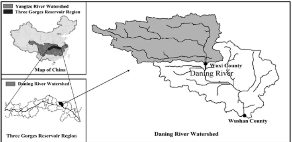
The Daning River Watershed (108◦44′–110◦11′E, 31◦04′–31◦44′N), lies in the cen-tral part of the Three Gorges Reservoir Area (TGRA) (Fig. 1), located in Wushan and Wuxi County, in the city of Chongqing, China, covering an area of 4426 km2. Mountain
5
makes up 95 % of the total area and low hills contributes the other 5 %. The aver-age altitude was 1197 m. The main landuse in the watershed include 22.2 % cropland, 11.4 % grassland, and 65.8 % forest. And zonal yellow soil is the dominant soil of the watershed. This area is characterized by the tropical monsoon and subtropical climate of Northern Asia. A humid subtropical monsoon climate covers this area, featuring
dis-10
tinct seasons with adequate illumination (an annual mean temperature of 16.6◦C) and abundant precipitation (an annual mean precipitation of 1124.5 mm). A hydrological station is located in Wuxi County, and this study focused on the watershed controlled by the Wuxi hydrological station, comprising of approximately 2027 km2(Fig. 1).
2.2 SWAT model
15
The SWAT (Arnold et al., 1998) model is a hydrologic/water quality tool developed by the United States Department of Agriculture-Agriculture Research Service (US-DAARS). The SWAT model is also available within the BASINS as one of the mod-els that the USEPA supports and recommends for state and federal agencies to use to address point and nonpoint source pollution control. The hydrological processes
20
HESSD
8, 8203–8229, 2011Analysis of parameter uncertainty in
hydrological
Z. Y. Shen et al.
Title Page
Abstract Introduction
Conclusions References
Tables Figures
◭ ◮
◭ ◮
Back Close
Full Screen / Esc
Printer-friendly Version Interactive Discussion
Discussion
P
a
per
|
Dis
cussion
P
a
per
|
Discussion
P
a
per
|
Discussio
n
P
a
per
|
Qsurf= Rday−Ia
2
Rday−Ia+S (1)
whereQsurf is the accumulated runoff or rainfall excess (mm H2O); Rday is the rain-fall depth for the day (mm H2O); Ia is the initial abstractions, which includes surface
storage, interception, and infiltration prior to runoff (mm H2O); andS is the retention parameter (mm H2O). The retention parameter varies spatially due to changes in soil,
5
land use, management, and slope and temporally due to changes in soil water content. The retention parameter is defined as:
S=25 400
CN −254 (2)
where CN is the curve number for the day.
The SWAT model uses the Modified Universal Soil Loss Equation (MUSLE) to
esti-10
mate sediment yield at HRU level. The MUSLE is defined as:
Qsed=11.8(Qsurf·qpeak·Ahru)0.56·Kusle·Cusle·Pusle·Lusle·FCFRG (3) whereQsedis the sediment yield on a given day (metric tons);Qsurfis the surface runoff
volume (mm H2O/ha);qpeakis the peak runoffrate (m3s−1);A
hruis the area of the HRU (Hydrological response units) (ha);Kusle is the USLE soil erodibility factor;Cusle is the
15
USLE cover and management factor;Pusle is the USLE support practice factor;Lusleis the USLE topographic factor; andFCFEG is the coarse fragment factor.
In order to efficiently and effectively apply the SWAT model, different calibration and uncertainty analysis methods have been developed and applied to improve the pre-diction reliability and quantify prepre-diction uncertainty of SWAT simulations (Arabi et al.,
20
HESSD
8, 8203–8229, 2011Analysis of parameter uncertainty in
hydrological
Z. Y. Shen et al.
Title Page
Abstract Introduction
Conclusions References
Tables Figures
◭ ◮
◭ ◮
Back Close
Full Screen / Esc
Printer-friendly Version Interactive Discussion
Discussion
P
a
per
|
Dis
cussion
P
a
per
|
Discussion
P
a
per
|
Discussio
n
P
a
per
the GLUE method. For modeling accurately, parameters were calibrated and validated using the highly efficient Sequential Uncertainty Fitting version-2 (SUFI-2) procedure (Abbaspour et al., 2007). The initial parameter range was recommended from SWAT manual. This calibration method is an inverse optimization approach that uses the Latin Hypercube Sampling (LHS) procedure along with a global search algorithm to
exam-5
ine the behavior of objective functions. The procedure has been incorporated into the SWAT-CUP software, which can be downloaded for free from the EAWAG website (Ab-baspour et al., 2009). For the runoff, the Nash-Sutcliffe coefficients during calibration period and validation period were 0.94 and 0.78. For the sediment yield, the Nash-Sutcliffe coefficients in calibration period and validation period were 0.80 and 0.70,
10
respectively. More details could be found in the study of Shen et al. (2008) and Gong et al. (2011).
2.3 GLUE method
The GLUE method (Beven and Freer, 2001) is an uncertainty analysis technique inspired by importance sampling and regional sensitivity analysis (Hornberger and
15
Spear, 1981). In GLUE, parameter uncertainty accounts for all sources of uncertainty, i.e., input uncertainty, structural uncertainty, parameter uncertainty and response un-certainty. Therefore, this method has been widely used in many areas as an effective and general strategy for model calibration and uncertainty estimation associated with complex models. In this study, the GLUE analysis process consists of the following
20
three steps:
Step 1: Definition of likelihood function
The likelihood function was used to evaluate SWAT outputs against observed values. In our study, Nash-Sutcliffe coefficient (NS) was picked because it’s the most frequently used likelihood measure for GLUE based on literature (Beven and Freer, 2001; Freer
HESSD
8, 8203–8229, 2011Analysis of parameter uncertainty in
hydrological
Z. Y. Shen et al.
Title Page
Abstract Introduction
Conclusions References
Tables Figures
◭ ◮
◭ ◮
Back Close
Full Screen / Esc
Printer-friendly Version Interactive Discussion
Discussion
P
a
per
|
Dis
cussion
P
a
per
|
Discussion
P
a
per
|
Discussio
n
P
a
per
|
et al., 1996; Arabi et al., 2007).
ENS=1−
n
P
i=1
Qsim,i−Qmea,i2
n
P
i=1
Qmea,i−Qmea2
(4)
Where Xi represents the outputs of time i, n represents the times, Qmea,i is the ob-served data,Qsim,i is the simulated data,Qmeais the mean value of the observed data, andnis the simulation time.
5
Step 2: Sampling parameter sets
Due to the lack of prior distribution of parameter, uniform distribution was chosen due to its simplicity (Lenhart et al., 2002; Muleta and Nicklow, 2005; Migliaccio and Chaubey, 2008). The range of each parameter was divided intonoverlapping intervals based on equal probability (Table 1) and parameters were identically chosen from spanning the
10
feasible parameter range. The drawback of typical GLUE approach was its prohibitive computational burden imposed by its random sampling strategy. Therefore in this study, an improved sampling method was introduced by combing Latin hypercube sampling (LHS). Compared to random sampling, LHS can reduce sampling times and provide 10-fold greater computing efficiency (Vachaud and Chen, 2002). Therefore, LHS was
15
used for random parameter sampling to enhance the simulation efficiency of the GLUE simulation. Values then were randomly selected from each interval.
If the initial sampling of the parameter space was not dense enough, GLUE sampling scheme probably could not ensure a sufficient precision of the statistics inferred from the retained solutions (Bates and Campbell, 2001). Hence, a large number of sampling
20
HESSD
8, 8203–8229, 2011Analysis of parameter uncertainty in
hydrological
Z. Y. Shen et al.
Title Page
Abstract Introduction
Conclusions References
Tables Figures
◭ ◮
◭ ◮
Back Close
Full Screen / Esc
Printer-friendly Version Interactive Discussion
Discussion
P
a
per
|
Dis
cussion
P
a
per
|
Discussion
P
a
per
|
Discussio
n
P
a
per
Step 3: Threshold definition and results analysis.
Compared to other applications (Gassman et al., 2007), 0.5 was judged as a reason-ableENSvalue for SWAT simulation. This study set 0.5 as threshold value ofENSand if the acceptability is below a certain subjective threshold, the run was considered to be “non-behavioral” and that parameter combination is removed from further analysis. In
5
this study, SWAT model was performed 10000 times with different parameter sample sets. For each output, the dotty plot, cumulative parameter frequency and 95CI were analyzed.
3 Results and discussion
3.1 Uncertainty of outputs
10
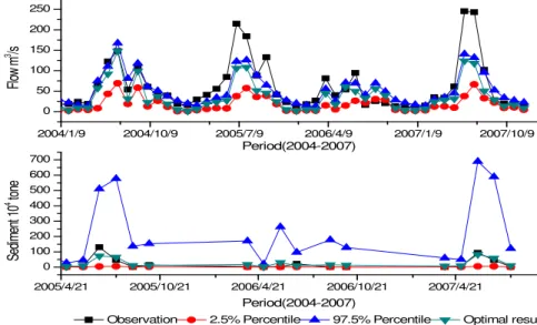
For the purpose of determining the extent to which parameter uncertainty affects model simulation, the degree of uncertainty of outputs was expressed by 95CI, which was derived by ordering the 10 000 outputs and then identifying the 2.5 % and 97.5 % threshold values. The 95CI for both stream flow and sediment period were shown in Fig. 2. It was evident that the 95CI of stream flow and sediment was 1∼53 m3s−1and
15
2000∼7 657 800 t, respectively. In addition, sediment simulation presented greater
un-certainty than stream flow, which might be due to the fact that sediment was affected and dominated by both stream flow processes as well as other factors such as land use variability (Shen et al., 2008; Migliaccio and Chaubey, 2008).
From Fig. 2, the temporal variation of outputs was presented in which it was evident
20
to obtain the clear relationship between the amount of the rainfall and the width of confidence interval. This result highlighted an increased model uncertainty in high precipitation condition. The variability in the uncertainty of sediment was the same as that for runoff, because runoff affects both factors. This could be explained by that uncertainty was inherent in precipitation due to variability in time of occurrence,
HESSD
8, 8203–8229, 2011Analysis of parameter uncertainty in
hydrological
Z. Y. Shen et al.
Title Page
Abstract Introduction
Conclusions References
Tables Figures
◭ ◮
◭ ◮
Back Close
Full Screen / Esc
Printer-friendly Version Interactive Discussion
Discussion
P
a
per
|
Dis
cussion
P
a
per
|
Discussion
P
a
per
|
Discussio
n
P
a
per
|
location, intensity, and tempo-spatial distribution (Shen et al., 2008). In hydrology model such as SWAT, although a rainfall event may affect only a small portion of the basin, the model assumes it affects the entire basin, which may cause a larger runoff
event was observed in simulation although little precipitation was recorded due to the limited local extent of certain precipitation event. In Three Gorges Reservoir area,
5
the daily stream flow changes frequently and widely, thus the monthly mean value of runoffmight not represent the actual change very well and the discrepancy between the measured mean value and simulated mean value would be high. Hence, daily precipitation data might be invalid in TGRA and more detailed precipitation data and stations should be obtained for hydrology modeling in TGRA.
10
From Fig. 2, it was clear that most of observation values were bracketed by the 95 CI, 54 % for stream flow outputs and 95 % for sediment. However, several stream flow observations were demonstrated above the 97.5 % threshold values (such as March, April, November in 2004; March, April, May, June, July, August and October in 2005; February, March, April, May and July in 2006; March, May, June, July and August in
15
2007). Conversely, only one observation (October in 2006) was observed below the 2.5 % threshold of sediment output. Measured value was not entirely in the range of 95CI, indicating that the SWAT model could not fully simulate the flow and sediment processes. However, it was acknowledged that from the parameter, model structure and data input also caused uncertainty in model simulation (Bates and Campbell, 2001;
20
Yang et al., 2007). Based on the results presented in this study, it was not possible to tell the extent to which the errors in the input and model structure contribute on the total simulation uncertainty. However, as parameter uncertainty was only able to account for a small part of whole uncertainty in hydrological modeling, this study suggested further studies on model structure and input in TGRA.
25
HESSD
8, 8203–8229, 2011Analysis of parameter uncertainty in
hydrological
Z. Y. Shen et al.
Title Page
Abstract Introduction
Conclusions References
Tables Figures
◭ ◮
◭ ◮
Back Close
Full Screen / Esc
Printer-friendly Version Interactive Discussion
Discussion
P
a
per
|
Dis
cussion
P
a
per
|
Discussion
P
a
per
|
Discussio
n
P
a
per
uncertainty in the estimated parameters in TGRA was obvious. This result agreed well with many other studies (Beven and Binley, 1992; Gupta and Sorooshian, 2005). This may due to the fact that parameters obtained from calibration were affected by several factors such as correlations amongst parameters, sensitivity or insensitivity in parame-ters, spatial and temporal scales and statistical features of model residuals (Wagener
5
et al., 2003; Wagener and Kollat, 2007). It could be inferred that the identifiability of optimal parameter obtained from calibration should also be evaluated. For an already gauged catchment, a virtual study can provide a point of reference for the minimum un-certainty associated with a model application. This study highlighted the importance of monitoring task for several important physical parameters to determine more credible
10
results for watershed management.
3.2 Uncertainty of parameters
Fig. 3 and Fig. 5 illustrated the variation ofENSfor Daing River watershed as a function of variation in each of the 20 parameters considered in this study. By observing the dotty plot from Fig. 3, it was evident that the main sources of streamflow uncertainty
15
were initial SCS CN II value (CN2), available water capacity of the layer (SOL AWC), maximum canopy storage (CANMX), base flow alpha factor for bank storage ( AL-PHA BNK), saturated hydraulic conductivity (SOL K), and soil evaporation compen-sation factor (ESCO). Among the above six parameters,SOL AWCandCANMX were the most identifiable parameters for Daing River watershed. This could be explained by
20
thatSOL AWCrepresented soil moisture characteristics or plant available water. This parameter played an important role in evaporation, which was associated with runoff
(Burba and Verma, 2005). It had also been suggested that the soil water capacity had an inverse relationship with various water balance components (Kannan et al., 2007). Therefore, an increase in theSOL AWC value would result in a decreased estimate
25
HESSD
8, 8203–8229, 2011Analysis of parameter uncertainty in
hydrological
Z. Y. Shen et al.
Title Page
Abstract Introduction
Conclusions References
Tables Figures
◭ ◮
◭ ◮
Back Close
Full Screen / Esc
Printer-friendly Version Interactive Discussion
Discussion
P
a
per
|
Dis
cussion
P
a
per
|
Discussion
P
a
per
|
Discussio
n
P
a
per
|
SOL K [80, 300] ) could also be obtained optimal parameter range using calibration method without much difficulties. However, presence of multiple peaks in the Nash-Sutcliffe model efficiency for CN2 and ESCO indicated that estimation of these pa-rameters might not be feasible.
However, it should be noted that non-identifiability of a parameter did not indicate that
5
the model was not sensitive to these parameters. Generally,CN2 was considered as the primary source of uncertainty when dealing with stream flow simulation (Eckhardt and Arnold, 2001; Lenhart et al., 2002). In this study, it showed that CN2 exhibited non-identifiability in stream flow simulation. This is similar to the study proposed by Kannan et al. (2006). The potential cause would be that there was an explicit
provi-10
sion in the SWAT model to update theCN2 value for each day of simulation based on available water content in the soil profile. Therefore, a change in the initialCN2 value would not greatly affect water balance components. Estimation of non-identifiable pa-rameters, such as CN2 and ESCO for Daning River watershed, would be difficult as there may be many combinations of these parameters that would result in similar model
15
performance.
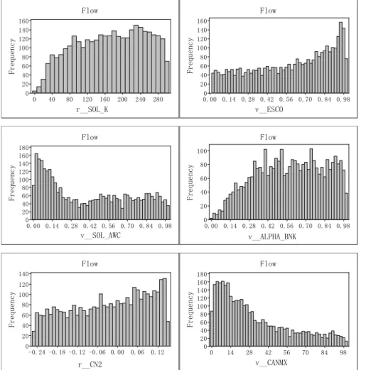
Figures 4 and 6 illustrated the cumulative parameter frequency for both stream flow and sediment in Daing River watershed. As shown in Fig. 4, the parameters were not uniformly or normally distributed, especially SOL AWC,CANMX and ESCO. ESCO
represented the influence of capillarity and soil cranny on soil evaporation in each
20
layer, a change in theESCO value therefore affected the entire water balance compo-nent. When there were higherESCOvalues, the estimated base flow, tile drainage and surface runoffincreased. The greater uncertainty of this parameter indicated that the soil evaporation probably played a greater role in the whole evaporation process, pos-sibly due to the high air temperature in TGRA. In comparison, other parameters such
25
HESSD
8, 8203–8229, 2011Analysis of parameter uncertainty in
hydrological
Z. Y. Shen et al.
Title Page
Abstract Introduction
Conclusions References
Tables Figures
◭ ◮
◭ ◮
Back Close
Full Screen / Esc
Printer-friendly Version Interactive Discussion
Discussion
P
a
per
|
Dis
cussion
P
a
per
|
Discussion
P
a
per
|
Discussio
n
P
a
per
important opinion that the model output was influenced by the set of parameter than a single parameter (Beven and Binley, 1992).
Similar to stream flow simulation, even though many of the parameters were sensi-tive and affected the sediment simulation, only a small number of the sensitive param-eters were identifiable. As shown in Fig. 5, the factors of uncertainty for sediment were
5
CN2, Manning’s value for main channel (CH N2), maximum canopy storage (CANMX), base flow alpha factor for bank storage (ALPHA BNK), exp.Re-entrainment parame-ter for channel sediment routing (SPEXP), lin.re-entrainment parameparame-ter for channel sediment routing (SPCON), channel cover factor (CH COV), channel erodibility factor (CH EROD). Clearly, the parameter samples were very dense around the maximum
10
limit (Fig. 6). From Figs. 3, 4, 5 and 6, it could be summarized that the parame-ters with greater uncertainty of stream flow mainly came from surface corresponding process and the parameters with greater uncertainty of sediment focused on channel response process. The results matched well with those of Yang et al. (2011) and Shen et al. (2010).
15
4 Conclusions
In this study, the GLUE method was employed to assess the parameter uncertainty in SWAT model applied in the Daning River Watershed of the Three Gorges Reservoir Region (TGRA), China. The results indicated that only a few of the parameters were sensitive and affected the stream flow and sediment simulation. It should be noted that
20
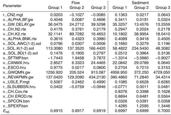
identifiable parameters such asCANMX,ALPHA BNK,SOL K could be obtained op-timal parameter range using calibration method without much difficulties. Conversely, presence of multiple peaks in non-identifiability parameters (CN2andESCO)indicated that calibration of these parameters might be feasible. In addition, multiple combina-tions of parameters contributed the same ENS during hydrologic modeling in TGRA.
25
HESSD
8, 8203–8229, 2011Analysis of parameter uncertainty in
hydrological
Z. Y. Shen et al.
Title Page
Abstract Introduction
Conclusions References
Tables Figures
◭ ◮
◭ ◮
Back Close
Full Screen / Esc
Printer-friendly Version Interactive Discussion
Discussion
P
a
per
|
Dis
cussion
P
a
per
|
Discussion
P
a
per
|
Discussio
n
P
a
per
|
should check if the final parameter values correspond to the watershed characteristics and its underlying hydrologic processes. It was anticipated this study would provide a practical and flexible implication for hydrology modeling related to policy development in the Three Gorges Reservoir Region (TGRA) and other similar areas.
It is suggested that more detailed measured data and more precipitation stations
5
should be obtained in the future for hydrology modeling in TGRA. And also further studies should be continued in the field of model structure and input to quantify hydrol-ogy model uncertainty in TGRA.
Acknowledgements. The study was supported by National Science Foundation for Distin-guished Young Scholars (No. 51025933), Program for Changjiang Scholars and Innovative 10
Research Team in University (No. IRT0809) and the Nonprofit Environment Protection Specific Project (No. 200709024).
References
Abbaspour, K. C., Yang, J., Maximov, I., Siber, R., Bogner, K., Mieleitner, J., Zobrist, J. and Srinivasan, R.: Modelling hydrology and water quality in the pre-alpine/alpine Thur watershed 15
using SWAT, J. Hydrol., 333, 413–430, 2007.
Arabi, M., Govindaraju, R. S., and Hantush M. M.: A probabilistic approach for analysis of uncertainty in the evaluation of watershed management practices., J. Hydrol., 333, 459–471, 2007.
Arnold, J. G., Srinivasan, R., Muttiah, R. S., and Williams, J. R.: Large area hydrologic modeling 20
and assessment part I: model development, J Am. Water Resour. As., 34, 73–89, 1998. Bates, B. C. and Campbell, E. P.: A Markov chain Monte Carlo scheme for parameter estimation
and inference in conceptual rainfall-runoffmodeling, Water Resour. Manag., 37, 937–947, 2001.
Beck, M. B.: Water quality modeling: A review of the analysis of uncertainty, Water Resour. 25
Manag., 23, 1393–1442, 1987.
HESSD
8, 8203–8229, 2011Analysis of parameter uncertainty in
hydrological
Z. Y. Shen et al.
Title Page
Abstract Introduction
Conclusions References
Tables Figures
◭ ◮
◭ ◮
Back Close
Full Screen / Esc
Printer-friendly Version Interactive Discussion
Discussion
P
a
per
|
Dis
cussion
P
a
per
|
Discussion
P
a
per
|
Discussio
n
P
a
per
Beven, K. J. and Freer, J.: Equifinality, data assimilation, and uncertainty estimation in mecha-nistic modeling of complex environmental systems, J. Hydrol., 249, 11–29, 2001.
Burba, G. G. and Verma, S. B.: Seasonal and interannual variability in evapotranspiration of native tallgrass prairie and cultivated wheat ecosystems, Agric. For. Meteorol., 135, 190–201, 2005.
5
Catari1, G., Latron, J., and Gallart, F.: Assessing the sources of uncertainty associated with the calculation of rainfall kinetic energy and erosivity – application to the Upper Llobregat Basin, NE Spain, Hydrol. Earth Syst. Sci., 15, 679–688, doi:10.5194/hess-15-679-2011, 2011. Cochrane, T. A. and Flanagan, D. C.: Effect of DEM resolutions in the runoff and soil loss
predictions of the WEPP watershed model, T ASAE, 48, 109–120, 2005. 10
Eckhardt, K. and Arnold, J. G.: Automatic calibration of a distributed catchment model, J. Hydrol., 251, 103–109, 2001.
Eckhardt, K., Breue, L. and Frede, H. G.: arameter uncertainty and the significance of simulated land use change effects, J. Hydrol., 273, 164–176, 2003.
Freer, J., Beven, K. and Ambroise, B.: Bayesian estimation of uncertainty in runoffprediction 15
and the value of data: an application of the GLUE approach, Water Resour. Res., 32, 2161– 2173, 1996.
Gassman, P. W., Reyes, M., Green, C. H., and Arnold J. G.: The soil and water assessment tool: historical development, applications, and future directions, T. ASAE, 50, 1212–1250, 2007.
20
Gong, Y. W., Shen, Z. Y., Hong, Q., Liu, R. M., and Liao, Q.: Parameter uncertainty analysis in watershed total phosphorus modeling using the GLUE methodology, Agr. Ecosyst. Environ., 142, 246–255, 2011.
Gupta, H. V., Beven, K. J., and Wagener, T.: Model calibration and uncertainty estimation. In: Anderson, M.G. (Ed.), Encyclopedia of Hydrological Sciences, John Wiley, New York, 25
2015–2031, 2005.
Hejberg, A. L. and Refsguard, J. C.: Model uncertainty-parameter uncertainty versus concep-tual models, Water Sci. Technol., 52, 177–186, 2005.
Hornberger, G. M. and Spear, R. C.: An approach to the preliminary analysis of environmental systems, J. Environ. Manage., 12, 7–18, 1981.
30
Jorgeson, J. and Julien, P.: Peak flow forecasting with radar precipitation and the distributed model CASC2D, Water Inter., 30, 40–49, 2005.
HESSD
8, 8203–8229, 2011Analysis of parameter uncertainty in
hydrological
Z. Y. Shen et al.
Title Page
Abstract Introduction
Conclusions References
Tables Figures
◭ ◮
◭ ◮
Back Close
Full Screen / Esc
Printer-friendly Version Interactive Discussion
Discussion
P
a
per
|
Dis
cussion
P
a
per
|
Discussion
P
a
per
|
Discussio
n
P
a
per
|
of the best evapotranspiration and runoffoptions for hydrological modelling in SWAT-2000, J. Hydrol., 332, 456–466, 2007.
Kao, J. J. and Hong, H. J.: NPS model parameter uncertainty analysis for an off-stream reser-voir, J. Hydrol., 32, 1067–1079, 1996.
Kingston, D. G. and Taylor, R. G.: Sources of uncertainty in climate change impacts on river 5
discharge and groundwater in a headwater catchment of the Upper Nile Basin, Uganda, Hydrol. Earth Syst. Sci., 14, 1297–1308, doi:10.5194/hess-14-1297-2010, 2010.
Lindenschmidt, K. E., Fleischbein, K., and Baborowski, M.: Structural uncertainty in a river water quality modelling system. Ecol. model., 204, 289–300, 2007.
Lenhart, T., Eckhardt, K., Fohrer, N., and Frede, H. G. Comparison of two different approaches 10
of sensitivity analysis, Phys. Chem. Earth, 27, 645-6-54, 2007.
Lu, X. X. and Higgitt, D. L.: Sediment delivery to the Three Gorges 2: Local response, Geo-morphology, 41, 157–169, 2001.
Melching, C. S. and Yoon, C. G.: Key sources of uncertainty in QUAL2E model of Passaic River, J Water Res. Pl.-ASCE, 122, 105–113, 1996.
15
Migliaccio, K. W. and Chaubey, I.: Spatial distributions and stochastic parameter influences on SWAT flow and sediment predictions, J Hydrol. Eng., 13, 258–269, 2008.
Miller, S. A. and Landisn A. E.: Theis TLUse of Monte Carlo analysis to characterize nitrogen fluxes in agroecosystems, Environ. Sci. Technol., 40, 2324–2332, 2006.
Muleta, M. K. and Nicklow, J. W.: Sensitivity and uncertainty analysis coupled with automatic 20
calibration for a distributed watershed model, J. Hydrol., 306, 127–145, 2005.
Murdoch, E. G. and Whelan, M. J.: Incorporating uncertainty into predictions of diffuse-source phosphorus transfers (using readily available data), Water Sci. Tech., 51, 339–346, 2005. Nandakumar, N. and Mein, R. G.: Uncertainty in rainfall-runoffmodel simulations and the
im-plications for predicting the hydrologic effects of land-use change, J Hydrol., 192, 211–232, 25
1997.
Quilbe, R., and Rousseau, A. N.: an integrated modelling system for watershed management – sample applications and current developments, Hydrol. Earth Syst. Sc., 11, 1785–1795, 2007.
Raat,K. J., Vrugt,J. A., Bouten, W., and Tietema, A.: Towards reduced uncertainty in catchment 30
nitrogen modelling: quantifying the effect of field observation uncertainty on model calibra-tion, Hydrol. Earth Syst. Sci., 8, 751–763, doi:10.5194/hess-8-751-2004, 2004.
HESSD
8, 8203–8229, 2011Analysis of parameter uncertainty in
hydrological
Z. Y. Shen et al.
Title Page
Abstract Introduction
Conclusions References
Tables Figures
◭ ◮
◭ ◮
Back Close
Full Screen / Esc
Printer-friendly Version Interactive Discussion
Discussion
P
a
per
|
Dis
cussion
P
a
per
|
Discussion
P
a
per
|
Discussio
n
P
a
per
Distributed Hydrology, Rosso R Peano A Becchi I, Bemporad GA (eds). Water Resources Publications: Fort Collins; 3–30, 1994.
Shen, Z. Y., Hong, Q., and Yu, H.: Parameter uncertainty analysis of the non-point source pollution in the Daning River watershed of the Three Gorges Reservoir Region, China, Sci. Total Environ., 405, 195–205, 2008.
5
Shen, Z. Y., Hong, Q., and Yu, H.: Parameter uncertainty analysis of non-point source pollution from different land use types, Sci. Total Environ., 408, 1971–1978, 2010.
Sohrabi, T. M., Shirmohammadi, A., Chu, T. W., Montas, H., and Nejadhashem, A. P.: Un-certainty Analysis of Hydrologic and Water Quality Predictions for a Small Watershed Using SWAT2000, Environ. Fore., 4, 229–238, 2003.
10
Sorooshian, S. and Gupta, V. K.: Model calibration. In Computer Models of Watershed Hy-drology, Singh VP (ed). Water Resources Publications: Highlands Ranch, Colorado, USA, 23–63, 1995.
Sudheer, K. P., Lakshmi, G., and Chaubey, I.: Application of a pseudo simulator to evaluate the sensitivity of parameters in complex watershed models, Environ. Modell. Softw., 26, 135– 15
143, 2011.
Van, G. A., Meixner, T., Srinivasan, R., and Grunwals, S.: Fit-for-purpose analysis of uncertainty using split-sampling evaluations, Hydrolog. Sci. J., 53, 1090–1103, 2008.
Vertessy, R. A., Hatton, T. J., Shaughnessy, P. J., and Jayasuriya, M. D.: Predicting water yield from a mountain ash forest catchment using a terrain analysis based catchment model, J. 20
Hydrol., 150, 665–700, 1993.
Vachaud, G. and Chen, T.: Sensitivity of a large-scale hydrologic model to quality of input data obtained at different scales; distributed versus stochastic non-distributed modeling, J. Hydrol., 264, 101–112, 2002.
Vazquez, R. F., Beven, K. and Feyen, J.: GLUE based assessment on the overall pre-dictions 25
of a MIKE SHE application, Water Resour. Manage., 23, 1325–1349, 2009.
Vrugt, J. A., Gupta, H. V., Bouten, W., and Sorooshian, S.: A shuffled complex evolution metropolis algorithm for optimization and uncertainty assessment of hydrologic model pa-rameters, Water Resour. Res., 39, 1201–1216, 2003.
Wagener, T. and Kollat, J.: Visual and numerical evaluation of hydrologic and environmental 30
models using the Monte Carlo Analysis Toolbox (MCAT), Environ. Modell. Softw., 22, 1021– 1033, 2007.
HESSD
8, 8203–8229, 2011Analysis of parameter uncertainty in
hydrological
Z. Y. Shen et al.
Title Page
Abstract Introduction
Conclusions References
Tables Figures
◭ ◮
◭ ◮
Back Close
Full Screen / Esc
Printer-friendly Version Interactive Discussion
Discussion
P
a
per
|
Dis
cussion
P
a
per
|
Discussion
P
a
per
|
Discussio
n
P
a
per
|
uncertainty in conceptual rainfall-runoff modeling: dynamic identifiability analysis, Hydrol. Process., 17, 455–476, 2003.
Wang, H. J., Yang, Z. S., Wang, Y., Saitom, Y., and Liu, J. P.: Reconstruction of sediment flux from the Changjiang (Yangtze River) to the sea since the 1860s, J. Hydrol., 349, 318–332, 2008.
5
Xu, H., Taylor, R. G., and Xu, Y.: Quantifying uncertainty in the impacts of climate change on river discharge in sub-catchments of the Yangtze and Yellow River Basins, China, Hydrol. Earth Syst. Sci., 15, 333–344, doi:10.5194/hess-15-333-2011, 2011.
Xuan, Y., Cluckie, I. D., and Wang, Y.: Uncertainty analysis of hydrological ensemble forecasts in a distributed model utilising short-range rainfall prediction, Hydrol. Earth Syst. Sci., 13, 10
293–303, doi:10.5194/hess-13-293-2009, 2009.
Yang, J., Reichert, P., and Abbaspour K. C., Xia, J. and Yang, H.: Comparing uncertainty analysis techniques for a SWAT application to the Chaohe Basin in China, J. Hydrol., 358, 1–23, 2008.
Yang, S. L., Zhao, Q. Y., Belkin, I. M.: Temporal variation in the sediment load of the Yangtze 15
River and the influences of human activities. J. Hydrol., 263, 56–71, 2002.
Zacharias, I., Dimitrio, E., and Koussouris, T. Integrated water management scenarios for wet-land protection: application in Trichonis Lake, Environ. Modell. Softw., 20, 177–185, 2005. Zhang, X.S., Raghavan, S., and David, B.: Calibration and uncertainty analysis of the SWAT
model using Genetic Algorithms and Bayesian Model Averaging, J. Hydrol.,374, 307–317, 20
HESSD
8, 8203–8229, 2011Analysis of parameter uncertainty in
hydrological
Z. Y. Shen et al.
Title Page
Abstract Introduction
Conclusions References
Tables Figures
◭ ◮
◭ ◮
Back Close
Full Screen / Esc
Printer-friendly Version Interactive Discussion
Discussion
P
a
per
|
Dis
cussion
P
a
per
|
Discussion
P
a
per
|
Discussio
n
P
a
per
Table 1.The range and optimal value of model parameter.
Name Lower limit Upper limit Optimal value
1 r CN2.mgt −0.25 0.15 −0.2143
2 v ALPHA BF.gw 0 1 0.6075
3 v GW DELAY.gw 1 45 13.4854
4 v CH N2.rte 0 0.5 0.2870
5 v CH K2.rte 0 150 36.1563
6 v ALPHA BNK.rte 0 1 0.1572
7 v SOL AWC.sol 0 1 0.0038
8 r SOL K.sol −0.2 300 251.4728
9 a SOL BD.sol 0.1 0.6 0.4442
10 v SFTMP.bsn −5 5 0.0499
11 v CANMX.hru 0 100 2.68
12 v ESCO.hru 0.01 1 0.5637
13 v GWQMN.gw 0 5000 3023.488
14 v REVAPMN.gw 0 500 380.7558
15 v USLE P.mgt 0.1 1 0.6443
16 v CH COV.rte 0 1 0.8124
17 v CH EROD.rte 0 1 0.0350
18 v SPCON.bsn 0 0.05 0.0210
19 v SPEXP.bsn 1 1.5 1.1924
HESSD
8, 8203–8229, 2011Analysis of parameter uncertainty in
hydrological
Z. Y. Shen et al.
Title Page
Abstract Introduction
Conclusions References
Tables Figures
◭ ◮
◭ ◮
Back Close
Full Screen / Esc
Printer-friendly Version Interactive Discussion
Discussion
P
a
per
|
Dis
cussion
P
a
per
|
Discussion
P
a
per
|
Discussio
n
P
a
per
|
Table 2.The equifinality of model parameters.
Parameter Group 1 Group 2Flow Group 3 Group 1 SedimentGroup 2 Group 3
r CN2.mgt 0.0203 −0.1027 −0.0085 0.1363 0.0217 0.0643
v ALPHA BF.gw 0.4048 0.0087 0.4896 0.3411 0.0191 0.0324
v GW DELAY.gw 36.0475 24.2712 39.5298 35.3257 13.4576 13.2559
v CH N2.rte 0.4176 0.3761 0.2179 0.2947 0.2024 0.2178
v CH K2.rte 32.1141 89.7282 16.4653 10.1802 38.9954 18.0410
v ALPHA BNK.rte 0.3616 0.4323 0.3980 0.4089 0.9418 0.4505
v SOL AWC(1-2).sol 0.0796 0.0307 0.0006 0.1660 0.3279 0.1196 r SOL K(1-2).sol 113.3080 137.3520 166.4420 58.4822 234.5450 48.3082 a SOL BD(1-2).sol 0.1476 0.1905 0.2797 0.2512 0.3964 0.3136 v SFTMP.bsn −1.7443 1.9458 3.7872 −1.3314 −3.5880 −0.9027
v CANMX.hru 2.8527 6.3323 24.4465 22.0842 29.0789 6.0640
v ESCO.hru 0.9775 0.0217 0.0800 0.2704 0.7215 0.3153
v GWQMN.gw 1256.920 205.524 913.087 4958.950 372.250 4729.050 v REVAPMN.gw 137.0420 129.2090 434.2130 390.4860 71.2840 34.4314
v USLE P.mgt 0.5067 0.2462 0.4990 0.1085 0.6628 0.6285
r SLSUBBSN.hru 0.0402 −0.0759 −0.0946 −0.0771 0.0011 0.0481
v CH Cov.rte 0.8376 0.3398 0.1628
v CH EROD.rte 0.8894 0.6481 0.5564
v SPCON.bsn 0.0326 0.0391 0.0358
v SPEXP.bsn 1.4285 1.2595 1.3446
HESSD
8, 8203–8229, 2011Analysis of parameter uncertainty in
hydrological
Z. Y. Shen et al.
Title Page
Abstract Introduction
Conclusions References
Tables Figures
◭ ◮
◭ ◮
Back Close
Full Screen / Esc
Printer-friendly Version Interactive Discussion
Discussion
P
a
per
|
Dis
cussion
P
a
per
|
Discussion
P
a
per
|
Discussio
n
P
a
per
|
2004/1/9 2004/10/9 2005/7/9 2006/4/9 2007/1/9 2007/10/9
0 50 100 150 200 250
2005/4/21 2005/10/21 2006/4/21 2006/10/21 2007/4/21
0 100 200 300 400 500 600 700
Fl
ow m
3 /s
Period(2004-2007)
Observation 2.5% Percentile 97.5% Percentile Optimal result
Sedi
m
ent
10
4 tone
Period(2004-2007)
HESSD
8, 8203–8229, 2011Analysis of parameter uncertainty in
hydrological
Z. Y. Shen et al.
Title Page Abstract Introduction Conclusions References Tables Figures ◭ ◮ ◭ ◮ Back Close
Full Screen / Esc
Printer-friendly Version Interactive Discussion Discussion P a per | Dis cussion P a per | Discussion P a per | Discussio n P a per 100 80 60 40 20 0 0.75 0.70 0.65 0.60 0.55 0.50 v__CANMX ENS Flow 5000 4000 3000 2000 1000 0 0.75 0.70 0.65 0.60 0.55 0.50 v__GWQMN EN S Flow 500 400 300 200 100 0 0.8 0.7 0.6 0.5 0.4 0.3 0.2 0.1 0.0
v _ _ R E V A P M N . g w _ 1
EN S Fl ow 100 80 60 40 20 0 0.8 0.7 0.6 0.5 0.4 0.3 0.2 0.1 0.0
v _ _ C A N M X . h r u _ _ _ _ _ _ _ _ 1 - 2 2
EN
S
F lo w
1.0 0.8 0.6 0.4 0.2 0.0 0.8 0.7 0.6 0.5 0.4 0.3 0.2 0.1 0.0
v _ _ S O L _ A W C ( 1 - 2 ) . s o l _ 1
EN S Fl ow 0.2 0.1 0.0 -0.1 -0.2 -0.3 0.75 0.70 0.65 0.60 0.55 0.50
r _ _ C N 2 . m g t
EN S Fl ow 500 400 300 200 100 0 0.75 0.70 0.65 0.60 0.55 0.50 v__REVAPMN EN S Flow 1.0 0.8 0.6 0.4 0.2 0.0 0.75 0.70 0.65 0.60 0.55 0.50 v__ALPHA_BNK EN S Flow 1.0 0.8 0.6 0.4 0.2 0.0 0.75 0.70 0.65 0.60 0.55 0.50 v__USLE_P EN S Flow 1.0 0.8 0.6 0.4 0.2 0.0 0.75 0.70 0.65 0.60 0.55 0.50 v_ALPHA_BF ENS Flow 160 140 120 100 80 60 40 20 0 0.75 0.70 0.65 0.60 0.55 0.50
v _ _ C H _ K 2 . r t e
EN S Fl ow 0.5 0.4 0.3 0.2 0.1 0.0 0.75 0.70 0.65 0.60 0.55 0.50
v _ _ C H _ N 2 . r t e
EN S Fl ow 300 250 200 150 100 50 0 0.75 0.70 0.65 0.60 0.55 0.50 r__SOL_K EN S Flow 0.6 0.5 0.4 0.3 0.2 0.1 0.75 0.70 0.65 0.60 0.55 0.50 a__SOL_BD EN S Flow 5.0 2.5 0.0 -2.5 -5.0 0.75 0.70 0.65 0.60 0.55 0.50 v__SFTMP EN S Flow 1.0 0.8 0.6 0.4 0.2 0.0 0.75 0.70 0.65 0.60 0.55 0.50 v__ESCO EN S Flow 0.5 0.4 0.3 0.2 0.1 0.0 0.75 0.70 0.65 0.60 0.55 0.50 v_CH_N2 EN S Flow 0.5 0.4 0.3 0.2 0.1 0.0 0.75 0.70 0.65 0.60 0.55 0.50 v_CH_N2 EN S Flow 50 40 30 20 10 0 0.75 0.70 0.65 0.60 0.55 0.50 v_GW_DELAY EN S Flow 1.0 0.8 0.6 0.4 0.2 0.0 0.75 0.70 0.65 0.60 0.55 0.50 v_SOL_AWC EN S Flow 0.2 0.1 0.0 -0.1 -0.2 -0.3 0.75 0.70 0.65 0.60 0.55 0.50 r_CN2 EN S Flow
HESSD
8, 8203–8229, 2011Analysis of parameter uncertainty in
hydrological
Z. Y. Shen et al.
Title Page Abstract Introduction Conclusions References Tables Figures ◭ ◮ ◭ ◮ Back Close
Full Screen / Esc
Printer-friendly Version Interactive Discussion Discussion P a per | Dis cussion P a per | Discussion P a per | Discussio n P a per | 280 240 200 160 120 80 40 0 160 140 120 100 80 60 40 20 0 r__SOL_K Frequency Flow 0.98 0.84 0.70 0.56 0.42 0.28 0.14 0.00 160 140 120 100 80 60 40 20 0 v__ESCO Frequency Flow 0.98 0.84 0.70 0.56 0.42 0.28 0.14 0.00 180 160 140 120 100 80 60 40 20 0 v__SOL_AWC Frequency Flow 0.98 0.84 0.70 0.56 0.42 0.28 0.14 0.00 100 80 60 40 20 0 v__ALPHA_BNK Frequency Flow 0.12 0.06 0.00 -0.06 -0.12 -0.18 -0.24 140 120 100 80 60 40 20 0 r__CN2 Frequency Flow 98 84 70 56 42 28 14 0 180 160 140 120 100 80 60 40 20 0 v__CANMX Frequency Flow
HESSD
8, 8203–8229, 2011Analysis of parameter uncertainty in
hydrological
Z. Y. Shen et al.
Title Page Abstract Introduction Conclusions References Tables Figures ◭ ◮ ◭ ◮ Back Close
Full Screen / Esc
Printer-friendly Version Interactive Discussion Discussion P a per | Dis cussion P a per | Discussion P a per | Discussio n P a per 0.2 0.1 0.0 -0.1 -0.2 -0.3 0.80 0.75 0.70 0.65 0.60 0.55 0.50 r__CN2 ENS Sediment 50 40 30 20 10 0 0.80 0.75 0.70 0.65 0.60 0.55 0.50 v__GW_DELAY ENS Sediment 160 140 120 100 80 60 40 20 0 0.80 0.75 0.70 0.65 0.60 0.55 0.50 v__CH_K2 ENS Sediment 1.0 0.8 0.6 0.4 0.2 0.0 0.80 0.75 0.70 0.65 0.60 0.55 0.50 v__SOL_AWC ENS Sediment 0.6 0.5 0.4 0.3 0.2 0.1 0.80 0.75 0.70 0.65 0.60 0.55 0.50 a__SOL_BD ENS Sediment 5.0 2.5 0.0 -2.5 -5.0 0.80 0.75 0.70 0.65 0.60 0.55 0.50 v__SFTMP ENS Sediment 1.0 0.8 0.6 0.4 0.2 0.0 0.80 0.75 0.70 0.65 0.60 0.55 0.50 v__ESCO ENS Sediment 500 400 300 200 100 0 0.80 0.75 0.70 0.65 0.60 0.55 0.50 v__REVAPMN ENS Sediment 1.0 0.8 0.6 0.4 0.2 0.0 0.80 0.75 0.70 0.65 0.60 0.55 0.50 v__CH_COV ENS Sediment 0.05 0.04 0.03 0.02 0.01 0.00 0.80 0.75 0.70 0.65 0.60 0.55 0.50 v__SPCON ENS Sediment 0.10 0.05 0.00 -0.05 -0.10 0.80 0.75 0.70 0.65 0.60 0.55 0.50 r__SLSUBBSN ENS Sediment 300 250 200 150 100 50 0 0.80 0.75 0.70 0.65 0.60 0.55 0.50 r__SOL_K ENS Sediment
HESSD
8, 8203–8229, 2011Analysis of parameter uncertainty in
hydrological
Z. Y. Shen et al.
Title Page Abstract Introduction Conclusions References Tables Figures ◭ ◮ ◭ ◮ Back Close
Full Screen / Esc
Printer-friendly Version Interactive Discussion Discussion P a per | Dis cussion P a per | Discussion P a per | Discussio n P a per | 0.12 0.06 0.00 -0.06 -0.12 -0.18 -0.24 100 80 60 40 20 0 r__CN2 Frequency Sediment 140 120 100 80 60 40 20 0 160 140 120 100 80 60 40 20 0 v__CH_K2 Frequency Sediment 0.98 0.84 0.70 0.56 0.42 0.28 0.14 0.00 80 70 60 50 40 30 20 10 0 v__SOL_AWC Frequency Sediment 98 84 70 56 42 28 14 0 70 60 50 40 30 20 10 0 v__CANMX Frequency Sediment 0.98 0.84 0.70 0.56 0.42 0.28 0.14 0.00 90 80 70 60 50 40 30 20 10 0 v__CH_COV Frequency Sediment 0.98 0.84 0.70 0.56 0.42 0.28 0.14 0.00 80 70 60 50 40 30 20 10 0 v__CH_EROD Frequency Sediment 0.049 0.042 0.035 0.028 0.021 0.014 0.007 0.000 90 80 70 60 50 40 30 20 10 0 v__SPCON Frequency Sediment 1.47 1.40 1.33 1.26 1.19 1.12 1.05 80 70 60 50 40 30 20 10 0 v__SPEXP Frequency Sediment