www.ocean-sci.net/6/285/2010/
© Author(s) 2010. This work is distributed under the Creative Commons Attribution 3.0 License.
Ocean Science
On contribution of horizontal and intra-layer convection to the
formation of the Baltic Sea cold intermediate layer
I. Chubarenko and N. Demchenko
P. P. Shirshov Institute of Oceanology RAS, Atlantic Branch, 236 000 Prospect Mira, 1, Kaliningrad, Russia Received: 7 October 2008 – Published in Ocean Sci. Discuss.: 24 November 2008
Revised: 11 January 2010 – Accepted: 11 February 2010 – Published: 26 February 2010
Abstract. Seasonal cascades down the coastal slopes and intra-layer convection are considered as the two additional mechanisms contributing to the Baltic Sea cold intermediate layer (CIL) formation along with conventional seasonal ver-tical mixing. Field measurements are presented, reporting for the first time the possibility of denser water formation and cascading from the Baltic Sea underwater slopes, which take place under fall and winter cooling conditions and deliver waters into intermediate layer of salinity stratified deep-sea area. The presence in spring within the CIL of water with temperature below that of maximum density (Tmd) and that at the local surface in winter time allows tracing its forma-tion: it is argued that the source of the coldest waters of the Baltic CIL is early spring (March–April) cascading, arising due to heating of water before reaching the Tmd. Fast in-crease of the open water heat content during further spring heating indicates that horizontal exchange rather than direct solar heating is responsible for that. When the surface is cov-ered with water, heated above the Tmd, the conditions within the CIL become favorable for intralayer convection due to the presence of waters of Tmd in intermediate layer, which can explain its well-known features – the observed increase of its salinity and deepening with time.
1 Introduction
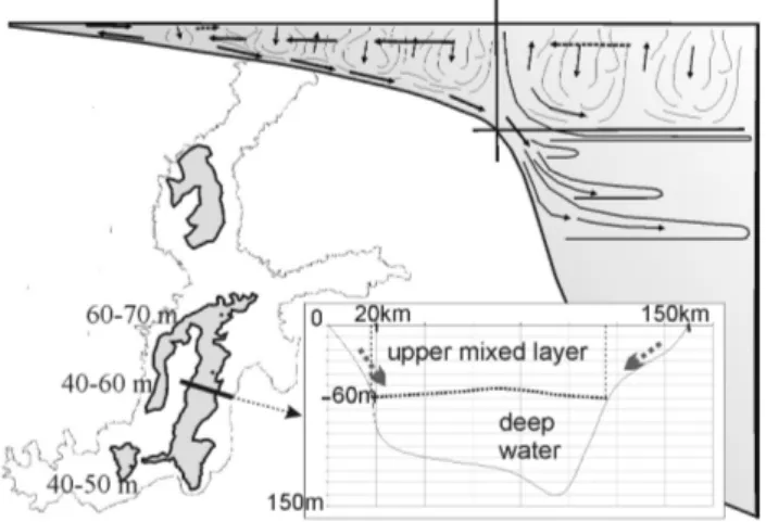
In the Baltic Sea, with its mean depth of about 50 m (Hy-drometeorology and hydrochemistry. . . , 1992; hereinafter – HH92), seasonal vertical convection in winter reaches the depths of 40 m (at the SW) to 60 m (at the NE). This means, that over ca. 60% of the area it reaches the bottom (Fig. 1). Over variable bottom topography, shallow areas cool faster
Correspondence to: I. Chubarenko (irina [email protected])
than deeper ones, resulting in more or less permanent hori-zontal gradients of temperature/density and subsequent cool down-slope currents. In the beginning of the cooling process in autumn, the flow follows day/night rhythm and is intermit-tent, characterized by “slugs” of colder water, moving one-by-one from the shore, and plunging underneath the upper mixed layer, into the thermocline – to meet the level of the corresponding density (see, for example, Fer et al., 2002a). This seasonal horizontal convective exchange is shown to be a very efficient mechanism of mixing in lakes and oceans (Farrow, 2004; Fer et al., 2002b; Imboden and W¨uest, 1995; Sturman et al., 1999; Killworth, 1977; Bennett, 1971; Thom-sen et al., 2001); however, to the authors’ knowledge, it was not yet observed in or applied for the conditions of the Baltic Sea. Being physically similar to the cascading in lakes, the process in sea environment is influenced by vertical and hori-zontal haline stratification. Sharing features with the oceanic “winter cascading from the shelf” (e.g., Killworth, 1977; Ja-cobs and Ivey, 1998), the cascading in the Baltic Sea is more complicated because twice per year the water temperature crosses the temperature of maximum density (Tmd), which never happens in saline oceanic water. At the same time, similar to fresh-water Lake Baikal, deep waters in the Baltic remain always above the Tmd due to their higher salinity, whilst the upper layer is cooled down to the freezing point (Shimaraev and Granin, 1991; W¨uest et al., 2005). In spite of all the differences, application of knowledge about oceanic and lake processes can shed some light onto the situation in the Baltic Sea.
Fig. 1. Map of the Baltic Sea, showing the regions (in dark), where winter vertical convection does not reach bottom (numbers show the maximum depth of the upper mixed layer, (HH92). Upper right scheme illustrates the mechanism of seasonal horizontal convective exchange between littoral area, where vertical convection reaches the bottom, and the open sea. The inset shows the bathymetry cross-section from Liepaja to Gotland with two 20–30 km long littoral slopes, where vertical convection reaches the bottom, separated by about 100 km-long deep-water portion.
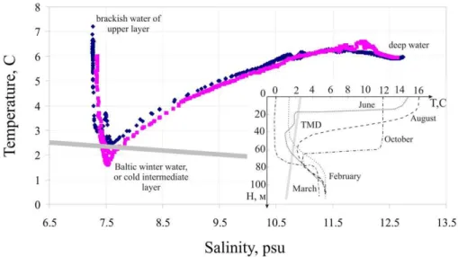
Feistel, 2007), is a water mass, located between the surface and the deep waters, typically at depths of about 40–60 m. It is easily identifiable in summer time by its low temperature (Fig. 2). The CIL is not a permanent feature. It is assumed (HH92; SEBS2008), that CIL develops in spring (March) with the formation of a seasonal thermocline, is most pro-nounced in summer time, and vanishes by the end of Novem-ber, together with the seasonal thermocline (Fig. 2). CIL reaches its maximum thickness (of about 30–40 m) in spring, when it is observed all over the Baltic area where the water depth is more than 60 m. The axis of the CIL (defined by the depth of the minimum water temperature; HH92) in spring is located at the depth of about 40–50 m. In summer, thickness of the layer somewhat decreases (to 20–30 m), and the axis deepens down to the 50–60 m. In autumn, thickness of the CIL is not more than 20 m, and the axis reaches it maximum depth (at about 60 m) (HH92).
Along with the lower temperature, high oxygen content and homogeneous salinity (0.1–0.4 higher than that of the upper layer) are typical features of the CIL (HH92). TS-diagram of Fig. 2 shows CIL as a water mass distinguished from the surface and bottom waters. Thus, the CIL can not be formed as a simple mixture of the latter two: the points representing such mixtures (at any proportion) should lie on a straight line between the surface and the deep water end members (Mamaev, 1975). An additional mechanism is re-quired to explain the formation of the CIL.
Two opinions are commonly expressed in this regard: (i) CIL is the remnant of the autumn-winter vertical
con-vection, capped by heated lighter water in summer; (ii) CIL is advected horizontally to deep parts of the Baltic Proper from its northern areas – the Bothnian Sea or the Bay of Finland. The first hypothesis explains why CIL is so fresh (oxygenated), however, does not explain why it is colder than the winter surface (e.g., monthly mean temperature – averaged over 30 years – in the Bornholm basin in March is 1.53◦C at the surface and only 1.5◦C at the depth of 30 m;
HH92), and why it is 0.1–0.4 saltier than the surface water (HH92). The second point of view, explaining the fact of coldness, fails to provide any reasons for heightened oxygen and salt content. Indeed, waters in the northern Baltic are less saline than in the Baltic Proper, and their way from so dis-tant regions (many hundreds of kilometres) with the speed of about 6–9 cm s−1(reported for the intermediate layer; HH92)
should last for about a year, so that the oxygenation would be much lower and at least its gradual decrease from north-east to south-west would be formed. But it is definitely not observed: waters of CIL in the Bornholm deep are as oxy-genated as in Gotland deep or everywhere further north. This indicates that these waters were at the surface roughly at the same time. We consider here the possibility of generation of these waters at the bottom slopes of neighbouring shal-low areas, as a result of seasonal differential cooling/heating process.
Fig. 2. Temperature-Salinity (TS) diagram derived using the IOW monitoring data for May of 2005 (blue) and 2006 (pink) at the Gotland deep. The Baltic Sea Cold Intermediate Layer (CIL) is identified. The inset shows the vertical temperature profiles for different months (HH92; after Piechura with changes, the Gulf of Gdansk). TS-diagram shows three principal water masses of the Baltic sea as the most distant points of the diagram, whilst quasi-linear portions correspond to waters formed by their mixing (see also Mamayev, 1975; Hagen and Feistel, 2007).
2 Autumn cooling and cascading down slopes in the Baltic Sea conditions
The cascading process is typically not believed to signifi-cantly influence the CIL formation because of several rea-sons. Before the all, coastal waters are usually more fresh, so that even lower temperature does not cause a density in-crease sufficient to slide down to the thermocline level. Sec-ond, the motions are driven by a very small horizontal density differences, so that wind-wave mixing may overshadow the convective flows. With these questions in mind, we analyze in this section (i) general structure of horizontal exchange due to cascading process and (ii) field data of an expedition to the Gdansk bay slopes. The conclusion is that horizontal water-exchange due to differential coastal cooling works in the Baltic Sea environment as well.
2.1 Autumn and winter cascading
The mechanism of generation of down-slope cascades is as follows (e.g., Fer et al.; 2002a, b; Horsh et al., 1994 and many others). In autumn, seasonal decrease of air temperature and difference between land and water-cooling rates cause a change in thermal regime of littoral waters (Forel, 1880; Mortimer, 1974). Instead of coastal water heating, observed typically in spring and summer periods, a differential coastal cooling develops in littoral lake/sea area. Cooling from the surface causes vertical thermo-gravitational convection in both deep and shallow areas. Because of the restricted water depth, most shallow and semi-enclosed areas cool faster than deeper ones. This leads to a permanent formation of slow
colder currents down the bottom slope towards the abyss, which sink down to the level of the corresponding density, underneath the mixed upper layer (Brooks et al., 1972; Im-boden and W¨uest, 1995; Britter et al., 1980; Garrett, 1991; Zhmur and Yakubenko, 2001; Fer et al., 2002b; Chubarenko and Hutter, 2005). The currents are driven by small density differences (1ρ/∼10−4−10−5), but their flow-rate increases
with down-slope distance, because of both entrainment and supply of additional portions of water cooled at the surface further offshore. Even though it was pointed out (Bennett, 1971; Carmack, 1979) that thermally induced seasonal hor-izontal mixing can be a very important mechanism of mat-ter and energy transport in lakes and inland seas with large shoals, not long ago it was still generally assumed that they contribute mainly to the mixing in the littoral area (Browand et al., 1987; Ellison and Turner, 1959).
Field investigations of last decades, however, have demon-strated both common presence of such cold-water cascades and “slugs” and their efficiency in horizontal transport and mixing, and obvious influence onto the basin-wide water dy-namics in large lakes and inland seas (Fer et al., 2002; Horsh et al., 1994; Leaman and Schott, 1991). In oceans, it has been proved already by field measurements that the intermediate and deep layers are formed by winter time surface cooling or brine rejection due to ice production at high latitudes (e.g., Foster et al., 1976; Killworth et al., 1977; Meincke, 1978; Thorpe and White, 1988; Leaman et al., 1991; Thomsen et al., 2001).
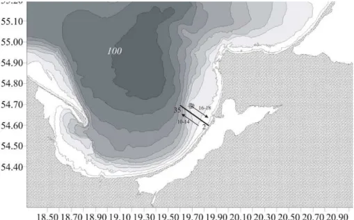
Fig. 3. Bathymetry of the Gdansk basin and the location of the experimental cross-section. Stations were numbered starting from the shore. Time of direct and back profiles are indicated.
bottom. The flow pattern is a combination of vertical convec-tive cells, down-slope density undercurrent and horizontal compensating flow (e.g., Chubarenko et al., 2005; CD2008), see Fig. 1. The most extensive field studies of seasonal cas-cading were performed in lakes (Fer et al., 2002a, b; Far-row and Patterson, 1993; Horsh et al., 1994; Sturman et al., 1999). All the observers point out the intermittent character of the flow and the “convective” behaviour of the horizontal water-exchange pattern.
Thus, if the goal is to estimate general structure of water-exchange and its overall influence, one should consider the large-scale features rather than instant flow characteristics. The situation is much alike with the Earth rotation: the Cori-olis force is small, but its influence is basin-wide. This way, coastal differential cooling/heating manifests itself in all the monthly averaged surface temperature maps (see, for exam-ple, HH92, SEBS2008 for the Baltic sea), even though par-ticular day/night or synoptic-scale pictures may be different. Still the principal question remains open: how the horizontal convective exchange is structured in sea environment, where coastal waters are often fresher than sea waters?
2.2 Expedition
2.2.1 Area description and environmental forcing
In order to investigate distinctive features of water ex-change, generated by differential cooling in the Baltic Sea coastal zone, an expedition was carried out by Laboratory for Coastal Systems Study of AB SIO and Department of Oceanography of Im. Kant State University (Kaliningrad) on 11–13 October 2006 in coastal zone of the Gulf of Gdansk
(see Fig. 3 for the map). Weather conditions were rather favourable. Almost calm and cold (11–12◦C) night before,
very low wind during the measurements (from 0 at the be-ginning to 5 ms−1 to the end), day time air temperatures
of 12–14◦C had provided a well pronounced surface
cool-ing conditions for sea waters of temperature of about 16◦C.
The overall cross-shore horizontal water temperature de-crease amounted to 0.7◦C/18 km, including 0.2◦C – colder
lens near the shore (see Figs. 4 and 5). With the observed air-water temperature difference of 1.2–4.3◦C and for wind
speed of ∼5 ms−1, an estimate for the value of the
turbu-lent heat-exchange isF∼10–30 W m−2. Solar radiation
dur-ing the entire day summed up to 90 Joule m−2, and
perma-nent cloudiness had smoothed its variation with time of the day. The resulting negative buoyancy fluxB=gαF
ρ0Cp had an
order of∼10−8m2s−3during the measurements (from 0900
to 1800). Here,α=−1/ρ0×∂ρ/∂T is water thermal
expan-sion coefficient, which is aboutα∼(1.72–1.79)×10−4◦C−1
for salinity of 7 psu. Fresher waters, out-flowing from the Vistula lagoon had in morning-time temperatures of about 14◦C, and upon the end of the expedition – to 15.5◦C, i.e.,
1–2◦C colder than seawater. Drifters put before the
mea-surements near the lagoon entrance indicated the main trans-port towards the north-north-west (current speed in the upper layer of about 20 cm s−1); so, in order to possibly avoid the
lagoon influence, the measurement polygon was chosen to be southward from the lagoon entrance. Still, data showed a remainder of colder (0.2◦C) and fresher (0.2 psu) surface
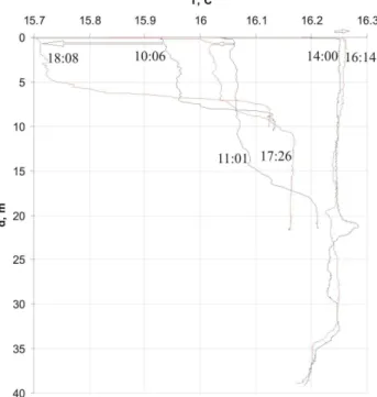
Fig. 4. Morning and afternoon vertical temperature profiles at St. 2, 11, 31 (see Fig. 3), demonstrating on-going coastal cooling.
2.2.2 Measurements
In all, 40 vertical CTD-profiles were performed during morning/day-time of 12 October along the line perpendicular to the shore. Bottom slope along the cross-section is variable: 0.0025 between St. 2 and St. 17 (9 km from the shore), 0.001 between St. 17 and St. 28 (9 km–14.5 km) and 0.0028 further down to the level where thermocline meets the slope. CTD-soundings were performed every 500 m from 4 m to 68 m depth, with total length of the cross-section of about 20 km. The profiles were numbered consequently from the shallow-most profile (number 2) to the deepest (number 35). Profile 1 was taken in the morning in the lagoon, and profiles 36–40 – on-shore in the afternoon. The probe, CTD 90M, provides the data with accuracy of 0.001◦C in temperature and 0.001
in salinity. Secchi depth, water colour and meteorological pa-rameters were registered, and water surface phenomena like streaks, foam, floating algae were monitored.
The main cross-section, containing 35 vertical profiles, was performed in offshore direction from 10:00 till 14:00 LT (local time) (i.e., GMT+2 h summer time). In order to reg-ister overall result of the day-time cooling, vertical profiles at three stations were repeated on the way back, from 16:15 till 18:00, using GPS in order to position the boat at the same very locations.
2.2.3 Results
Vertical temperature profiles of the morning and evening soundings are presented on Fig. 4, demonstrating a well pronounced differential coastal cooling during the mea-surement time. Shallow-most profiles (at the depth of 10 m) shows maximum cooling rate in the surface 5 m - thick layer – 0.22◦C/8 h∼0.028◦C/h; over the depth
of 21.5 m it amounts to 0.05◦C/6.5 h∼0.008◦C/h, and
over the depth of 39 m – a weak heating is indicated (0.004◦C/2 h∼0.002◦C/h), caused by water dynamics
de-scribed below. From simple heat balance of water column without advection, 1F=cpm1T, for the same heat loss 1F, the product of rate of cooling by the local depth di
should remain constant. However, comparing two shallow profiles, (0.028◦C/h×10 m)>(0.008◦C/h×21.5 m),
indicat-ing (i) presence of advection and (ii) higher additional ad-vective heat supply to the column at 21.5 m. This supply is provided by a compensating flow, which transports warmer open sea waters on-shore.
Vertical convective overturning over depths of several tens of meters and less works much faster than the cooling-induced horizontal advection over the length of the coastal slope (several tens of minutes versus many hours). For this reason, thermal variations due to variable depth arise faster than the corresponding advection develops - and smoothes them. This way, coastal cooling is formed readily – but is not at all directly connected to the corresponding currents. The arising flows by definition lag the imposed forcing (Far-row, 2004), and are actually driven by the density (not just temperature) gradients, what makes the situation in sea envi-ronment much more complicated than in fresh-water lakes. In the performed measurements, such a complication had arisen: the remainder of the Vistula lagoon plume influenced the density field near the shore. Detached already from the coast-line, it carried fresher and colder water. Resulting hor-izontal cross-shore temperature, salinity and density profiles for the second meter below the water surface are given on Fig. 5. They are obtained by extraction of corresponding por-tions (second meter under the surface) from individual ver-tical profiles and averaging over 1 m of the depth. All three profiles have the same shape, indicating a 3-km-long fresh-ened water lens near the shore-line. Without the colder lens, total cross-shore horizontal temperature difference amounted to 16.27–15.76◦C=0.53◦C/15 km∼0.035◦C/km. Salinity
decrease towards the shore makes up (again ignoring the lens) 7.05−6.97=0.08 psu/15 km∼0.005 psu/km. The re-sulting density increase towards the shore is as small as
1ρ/1x∼6×10−5 kg m−3/15 km=0.4×10⁻⁸kg m−3/m.
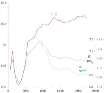
Fig. 5. Horizontal cross-shore temperature (red), salinity (blue) and in situ density anomaly (green) profiles, averaged for the second meter below the water surface, demonstrate coastal cooling and in-crease of density towards the shore. 3 km-long fresher and colder lens near the shore is the remainder of the Vistula lagoon plume.
Seasonal thermo/halo/pycno-cline was found to meet the bottom slope at the depth of about 41 m, with the tem-perature of the well pronounced upper mixed layer (UML) there of 16.2◦C. However, in the central part of the slope
(St. 19/depth 30 m and further down slope, see Figs. 7 and 8), temperature and salinity fields exhibit a 3-layered fine struc-ture. Easily identifiable upper homogeneous layer here has a thickness of mainly 0.52–0.62d (up to 0.73d once), where
d is the local depth. Below it, a warmer (+(0.02÷0.04)◦C
for deeper profiles 25-30, and up to+0.11◦C for St. 19)
and saltier (+0.1 psu in the central part to +0.15 psu to pro-file 30) layer is located, with the thickness of 0.36–0.23d
(once 0.1d, St. 25), what in absolute values is 13–7 m (once 3 m). And further below, a 3–8 m-thick layer of colder water is found along the bottom slope, with minimum water tem-perature of 16.02◦C (Fig. 7). Temperature in this bottom
layer is 0.1–0.2◦C lower than that of the UML, and 0.15◦C
– up to 0.2◦C (profile 25) lower than that in the middle layer.
Salinity of the bottom layer is very close to that of the middle layer; only at the deep-most slope St. 28–30, bottom salinity is up to 0.05 psu less than that in the middle layer.
In the shallow-most part of the section, a 7–8 m thick lens of lighter water is located. Even though it is colder (min-imum temperature is 15.62◦C versus 16.16◦C directly
be-low it at the bottom, depth 15.5 m), it is more fresh (mini-mum salinity 6.83 psu versus 7.11 psu), what results in a sta-ble density stratification with surface-bottom density differ-ence of 2×10⁻⁴kg m−3(for 15.5 m depth). Influence of the
Vistula lagoon waters is to be suggested immediately. La-goon water is typically of a salinity of 3–5 psu only, whilst
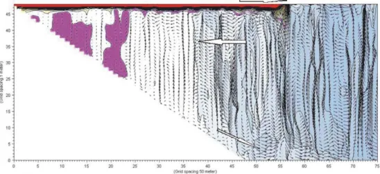
Fig. 6. Temperature, salinity and in situ density anomaly fields across the shore line, based at 35 vertical profiles (locations are marked by long ticks on upper panel). Surface 50 cm are removed. Solid isolines are drown every 0.1◦C/psu/kg m−3, short-dash iso-lines – for 0.05◦C/psu/kg m−3; other types of lines – for smaller
gradations – are to display features of finer structure. White arrows show a flow structure suggested by numerical and laboratory mod-elling and other field observations, and vertical red line – shows a border of the coastal dynamic cell.
the open sea waters are at the surface of a 7–7.2 psu. Thus (estimative), to become 6.85 psu saline, the lagoon water of 5 psu should be mixed withn=(6.85−5)/(7.1−6.85)=7.4 vol-umes of 7.1-psu-marine water. Taking into account rather calm weather conditions, distance from the lagoon entrance (∼5 km), general north-north-western transport in coastal zone, indicated by surface drifters, it is logical to consider these waters as already significantly assimilated by the on-going thermal and dynamic processes in sea coastal zone.
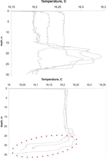
Fig. 7. Vertical temperature profiles: (a) in the middle part of the slope (St. 16, 19, 20, 21), (b) deep end of the slope (St. 25, 26, 28). Thermocline is at the depth of 41 m. Profiles (a) show gradual cooling towards the shore in the upper layer, colder waters at the bottom and warmer part in-between. Profiles (b) show much thicker cold layer (marked by the dotted circle).
of differential cooling and subsequent horizontal convec-tive processes in various set-ups. Numerical modelling for natural basins indicates (Chubarenko and Palij, 2006; Chubarenko et al., 2007), that in the top-most part of the slope currents tend to be two-dimensional in horizontal plane; further down – the flow is intermittent, and the “slugs” are formed following day/night rhythm; and only after a cer-tain depth – the flow gets a shape of near-bottom layer. In small-scale laboratory modelling, Farrow (2004) suggested, that there is a region where vertical thermal conduction plays the role rather than convection. In our laboratory experiments (CD2008), down-slope gravity current induces a compensat-ing on-shore flow, which meets the bottom slope at a cer-tain depth (about 1/3 of the depth of the convectively mixed layer) and causes an up-slope flow in shallowest area. In sea environment, lower salinity of littoral waters is a common
Fig. 8. Vertical profile at St. 19: temperature (red line), salin-ity (blue) and in situ denssalin-ity anomaly (black); the axes have the cor-responding colours. Salinity profile has 2-layered structure, whilst temperature profile shows upper mixed layer, warm interior and bot-tom layer of the temperature lower than that at the surface.
situation, and exactly this point is always an argument why these waters could not ventilate deep sea layers, in contrast to lakes. The presented field data may be considered as a com-mon for the sea environment example of the formation of the coastal region with a specific water dynamics as well. This study also demonstrates the mechanism of mixing which pro-duces waters, cold and saline at the same time.
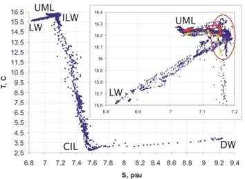
Fig. 9. TS representation of the field measurement data, showing water of lagoon origin (LW), water of the upper mixed layer (UML), water of the newly forming intermediate layer (ILW), the remainder of the CIL of the past year and deep Baltic water (DW). In insert, an enlarged upper part of the diagram is shown in more detail: points of profiles 25 and 26, containing cold bottom slugs, are highlighted in red and yellow, correspondingly.
At St. 29, the temperature maximum (and, presumably, the “nose” of warm thermal intrusion) is at 27 m (0.79d), fur-ther upslope (to St. 25, 22, 21, 20) it gradually lifts up, almost keeping the relative depth, decreasing only slightly from 0.76d (St. 25) to 0.74d (St. 20). The thickness of the compensating flow (again as deduced from the CTD profiles) is about (1/3–1/4)d in the lower half of the slope.
Near the 21–27 m isobaths (St. 12–15; about 7 to 9 km from the shore), where the compensating flow meets the slope, a large mixed region resembling a convective chimney is observed. Water column is homogeneous in both salinity (7.15 psu) and temperature (16.15◦C) down to the bottom,
while on the both sides water is vertically stratified. Wa-ter is the densest here (see Fig. 6, lower panel), and the iso-pycnals are sloping down on both sides. One can see “slugs” (Fer et al., 2002a, b), presumably moving to both sides from this mixing region. That “moving upslope” are warmer and saltier than waters around them; they form a “continuation” of the compensating flow. The slugs moving down-slope are colder, than overlying waters, and of almost the same salin-ity (in deep areas sometimes just a few hundredth less). The thickness of the down-flow is variable (see upper panel of Fig. 6): 3.5 m at St. 19, 7.5 m at St. 25, and further down-slope (St. 29, 30, 31) the lowest 16–20 m have complicated stratification, containing 2 warmer and 2 colder layers (this is still well above the thermocline in deep area!). The colder layers are 7 m and 5 m-thick. Thus, in the middle part of the slope, lower 0.1–0.15 d are occupied by colder waters, and to the end of the slope this layer grows up to 0.3 d. This is in full agreement with our laboratory experiments (Chubarenko et al., 2005), and less than 0.43 d, predicted by numerical
modelling of Horsh and Stefan (1988) for laboratory condi-tions.
Thus, overall structure of water exchange during the ex-periment can be interpreted as follows. Coastal differential cooling and weak off-shore wind established an off-shore water transport in bottom and surface layer, with a com-pensating flow formed in the lower half of the UML. In deeper areas, this flow is centered at about 0.75 of the depth of thermocline, and when approaching the slope, it slightly upwelled to about 0.75 of the local depth. Finally, at the depth of about half the depth of the thermocline in deep area, large (2–3 km along the slope) mixing region occurs, where colder/fresher littoral waters are mixed with saltier/warmer marine waters.
The described picture of mixing is in accord with on-board observations of water transparency and surface fea-tures. Starting from the depths of about 18 m, many medusas appeared, and water transparency abruptly increased from 4.5 m to 6.5 m – indicating transition to sea waters. Even though wind was rather weak (2–3 m s−1), foam flakes were
observed over a large fraction of the sea surface. In the mix-ing region (over 21–31 m isobaths), only separated flakes are registered, whilst closer to the shore (14–20 m), regu-lar down-wind rows with about 3–4 m spacing, and farther off-shore (33–40 m), with much larger separation (15–20 m) were observed. In the regions deeper than 40 m, foam flakes were not organized in rows. These observations corroborate that (i) the surface cooling conditions favour the formation of windrows, and that the wind rows, under convective condi-tions, can appear even under very weak wind; (ii) there was an off-shore flow in upper layer. The onshore return flow in middle layer therefore brings waters to compensate for both the cold slugs and the surface transport. Albeit the lagoon influence and relatively mild autumn cooling, data show that littoral area is “leaking” colder (0.1–0.2◦C) water (with
prac-tically the same salinity as UML) in a 0.1–0.3Dthick bottom layer.
TS plot derived from all profiles (Fig. 9) suggests that five water masses interact: the most freshened water of lagoon origin (LW), water of the upper mixed layer – with slightly varying temperature due to coastal differen-tial cooling (UML), water of the newly formed intermedi-ate layer (ILW), the remainder of the CIL of the past year and deep Baltic water (DW). The profiles with bottom slugs (St. 25 – in red, and St. 26 – in yellow) in inset of Fig. 9 show bottom waters colder than UML with about the same (and uniform) salinity. Thus, the points showing the slugs’ properties are located at the bend of the TS-diagram, which – with further cooling – can be modified to CIL.
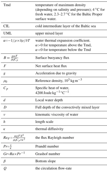
Table 1. List of main symbols and abbreviations.
Tmd temperature of maximum density
(depending on salinity and pressure); 4◦C for
fresh water, 2.3–2.7◦C for the Baltic Proper surface water.
CIL cold intermediate layer of the Baltic sea
UML upper mixed layer
α=−1/ρ×∂ρ/∂T water thermal expansion coefficient.
α>0 for temperature above the Tmd,
α<0 for temperature below the Tmd
B=ρgαF
0Cp Surface buoyancy flux
F Net surface heat flux
g Acceleration due to gravity
ρ0 Reference density, 103kg m−3
Cp Specific heat of water,
4200 Joule kg−1◦C−1
d Local water depth
D Full depth of the convectively mixed layer
ν kinematic viscosity of water
h length scale
κ thermal diffusivity
RaF= αgF h
4
ρ0Cpνκ2 the flux Rayleigh number
Pr=νκ Prandtl number
Gr=Ra×Pr−1 Grashof number
β Bottom slope
Q the circulation flow-rate
probable, this lowering is the result of the flow adjustment to an existence of freshened coastal wedge waters. Compen-sating on-shore flow of warmer/saltier sea water meets the slope over the depths of about 0.5–0.7 of the UML-depth and causes a large mixing region, which is the source of relatively cold and salty bottom ‘slugs’. Waters within these “slugs” are no longer the “coastal” ones: they are much warmer and saltier; they are rather “slope waters”, and are represented by their specific cloud at TS-diagram.
3 Spring heating and cross-over the Tmd
3.1 Early-spring cascading
Recent investigations of Hinrichsen et al. (2007) have demonstrated an important feature: the highest (up to 0.8– 0.9) annual-mean correlation between the temperatures of the CIL and the surface water is in March (data set of 1950–2005
Fig. 10. Temperature, salinity, in situ density anomaly and temper-ature of maximum density (depending on salinity and depth) in the Gotland basin on 7 May 2006. The corresponding TS-diagram with Tmd-line is presented in insert. (IOW monitoring data base).
was analyzed). Note, that the lowest CIL water tempera-tures are slightly below the lowest surface water temperatempera-tures in the same area, what is also statistically proved indepen-dently by Russian (HH92 – monthly mean for 30 years) and Swedish data (national atlas “Sea and coast”, p. 60, SMHI; 10-years averaging). Consider general hydrological condi-tions in the Baltic over late winter – early spring period.
Winter cooling below Tmd leads in the Baltic to a forma-tion of an inverse vertical temperature stratificaforma-tion in upper 10–15 m, which is, however, often easily destroyed by wind mixing down to the seasonal pycnocline at 40–60 m (HH92; SEBS2008). Mean-monthly surface temperature in March is 1.6–2.3◦C in central Baltic (SEBS2008); in field
exam-ple of Fig. 1 (Gdansk basin) – surface temperature is around 0◦C. Thus, when the surface heat balance becomes positive
(by mid-March in the central Baltic; HH92; SEBS2008), sur-face waters (typically) everywhere in the Baltic are below the Tmd, and remain so until the middle/end of April (in the SW part) and middle of May (NE part). Physically, such condi-tions are equivalent to autumn cooling process, considered above: the buoyancy fluxB=gαF
ρ0Cp into the surface layer is
Fig. 11. Vertical cross-section of simulated temperature and velocity fields for heating from the surface of an initially homogeneous layer (depth 50 m, length 4 km, width 10 km) fromT <Tmd. Pink colour marks the region with temperature of maximum density; blue region is still below, whilst yellow and red one – already above the Tmd. Isotherms are plotted every 0.058◦C, and are omitted above 5◦C
(in the upper-most layer). Velocity vectors show vertical convection due to positive bouyancy flux from above in the entire region with T <Tmd, including waters below the warm surface jet. The largest velocities are of the order of 2–3 cm/s; no scaling is applied to the vertical component. Large white arrows show mean horizontal transport. Heating is modelled as turbulent heat exchange with warmer air and solar heating, corresponding to spring period at mid latitudes, with day-night variations. The simulation is performed by MIKE3-FlowModel (DHI – Water and Environment).
α<0, F >0 (in spring; for the meaning of symbols see Ta-ble 1). Detailed laboratory experiments of a basin with slop-ing sides under such conditions are described in (CD2008). This way, early spring heating can also trigger comparable cascades. For the Baltis sea conditions, these warm-water cascades (which are warmer than the UML, but still be-low the Tmd) have 1 to 2 months to develop, until the sur-face water is heated up to the Tmd. The process of grad-ual heating has again the same logic: shallow waters heat faster, become denser and flow downslope. Hydro-physical field data, obtained in March in coastal zone, indicate both warm-water (denser) slugs on the sloping bottom and two-three-layered structure (like on Figs. 7–8) of vertical profiles over slopes (cruises of r/v “Professor Stokman”: no. 59, 3– 9 March 2004 and no. 67, 2–7 March 2005). Comparative analysis of data of several such spring cruises, presented in Morozov et al. (2007), says that horizontal temperature gra-dients are typical in March for coastal regions, and more in-tense heating in shallow areas may in some years generate a front along the shelf break.
Field data on the spring cascades, to the authors’ knowl-edge, are not yet reported in literature. We may only sug-gest that the cold bottom intrusions observed in Lake Baikal (W¨uest et al., 2005), are formed this way: the authors relate the phenomenon with the spring thermal bar, and point out that “the source of the regularly occurring deep intrusions is clearly cold surface water, but the actual mechanism is un-certain”.
In fact, the very “cascading” (when denser water flows down-slope with a considerable velocities, up to 5–8 cm/s;
Fer et al., 2002) is the least manifestation of the convective horizontal exchange. Horizontal convection has not a thresh-old, and waters start to move how only the smallest horizon-tal gradients arise. Wind mixing or currents of other origin may overshadow this exchange, but cannot stop it, and the observed cross-shore horizontal temperature differences dis-play the result of heat exchange with both the atmosphere and the sea. For the problem under discussion it is impor-tant, that horizontal exchange exists, and cold waters (below the Tmd), being heated in spring time over the Baltic slopes, can be used to trace it.
3.2 Crossing the Tmd
Shallow waters react faster on the change of heating condi-tions, they reach the Tmd sooner, whilst in deeper area ver-tical convection still mixes the newly-formed UML. Verti-cal convection should proceed and the thickness of the UML should increase as long as waters with T <Tmd are heated from above. Finally, if a certain water column is taken sepa-rately from the others, it should mix over the entire depth at the Tmd (feature known as a “spring overturning” in lakes) – and transfer to direct summer stratification, with the warmest waters on the top. Analysis of general hydro-physical condi-tions in the Baltic shows the following situation.
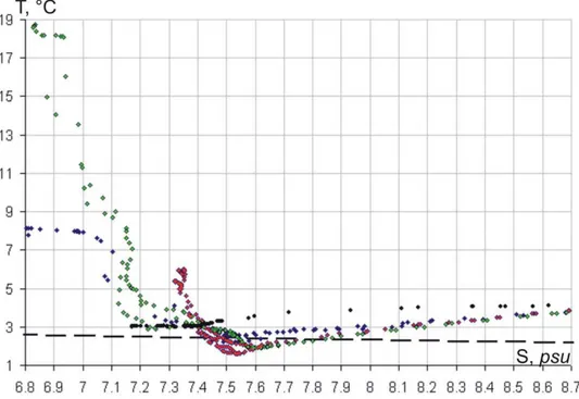
Fig. 12. TS-diagrams (for upper 60 m) in the Gotland basin in year 2006 (IOW monitoring data base): black points – for the end of January; red – for May; green – for July; blue – for November. Dashed line indicates the Tmd (T,S).
0◦C (see Fig. 2) to Tmd∼2.5◦C (for salinity 7 psu) is
F=Cp×ρ×D×1T∼4200×1000×60×2.5=6.3×10⁸Joule
m−2. This is about four times the heating from the beginning
of March to the end of April (crossing the Tmd by surface water in the central Baltic; HH92; SEBS2008). Note, that both the mean-annual data (HH92; SEBS2008) and the instant profiles (Figs. 2 and 10) show that in April, May, June, and some years in July, the surface is heated above the Tmd, whilst below this warm layer there is remnants of waters with temperature below the Tmd. As discussed above, such profile cannot be formed by local heating from the surface. Thus, the rapidly heated water should be advected from shallows (Fig. 11). This advected warm water covers the colder layer, isolating it from the solar heating. From this time on, the isolated cold water patch becomes the CIL.
In order to illustrate the structure of water-exchange, we present here a numerical simulation result (Fig. 11). The flow in an initially homogeneous (at 0◦C) fresh basin is
sim-ulated by the 3-dimensional baroclinic MIKE3-Flow model (DHI Water and Environment) using the non-hydrostatic en-gine (for more detail, see Chubarenko and Palij, 2006). The model basin of horizontal dimensions of 80×20 grid points (rectangular mesh 50 m×50 m) had 2.5 km-long (50 meshes) bottom slope of 0.02 and the depth of 50 layers (1 m each). External forcing was homogeneous over the surface, with air temperature of 10◦C, modulated by diurnal variations
of spring-time solar radiation typical at mid latitudes. Wind forcing was excluded.
On the picture, a numerical instant is shown when the up-per layer temup-perature is above the Tmd, whilst that in the deeper layer is below it, typical of the Baltic in May (see temperature profile in Gotland basin at Fig. 12). The shallow coastal region is vertically stably stratified and the vertical motions are suppressed. Over the rest of the slope, the water is still below the Tmd, thus, experiencing vertical convective mixing due to negative buoyancy flux either directly from the atmosphere or from the warmer advected water. The ver-tical mixing persists until Tmd is reached, and the horizontal exchange continues until at least some of this water (with
T <Tmd) is still in the region with sloping boundary. Impor-tant for further evolution of the CIL is that the warm surface jet, resulting from the horizontal pressure gradient in upper layers, does not change the mixing regime of the water body below it, and vertical convection continues until the waters are completely heated above the Tmd.
4 Summer-time evolution: intralayer convection
With much lower intensity, the process of denser water gen-eration over slopes should continue even when the CIL is al-ready covered by heated waters: diffusive heat flux from the surface layer becomes the source of destabilizing buoyancy flux now. Physically, it proceeds until at least some fraction of waters withT <Tmd is limited from below by the slop-ing bottom. Morozov et al. (2007) report field measurements of 52 cruise of r/v “Professor Stokman” (24–29 May 2003), performed in coastal zone near the Curonean spit (from the shore to 78 m depth), where cold water bodies (T <Tmd) are still over slope, well above the level of the CIL in open area. As long as the CIL comprises water below the Tmd in warm period, vertical temperature profile will cross the Tmd twice (see Fig. 10), thus providing conditions for the sort of thermobaric instability. This kind of instability was shown to be the reason for the formation of 120 m – thick homoge-neous layer around meso-thermal maximum in Lake Baikal (W¨uest, et al., 2005). In fresh-water Baikal, however, the Tmd varies with depth due to the pressure solely, whilst in the Baltic both pressure and salinity contribute to the Tmd variations with the depth. In the Baltic, at the initial cross of Tmd, heating from above causes mixing of the layer be-low it (i.e., of the CIL, with itsα<0); at the second cross of Tmd, instability arises because of cooling from above of the deeper waters, withα>0. Both mixing mechanisms work in the same direction: downward, mixing waters of the CIL itself and entraining deeper layers.
This agrees well with the observed CIL features: from spring to autumn, the axis of the CIL gradually deepens -from 40–50 m to about 60 m in central Baltic (HH92), while its salinity slightly increases. In order to show this more ev-idently, we plotted TS-diagrams of IOW monitoring of the Gotland basin in year 2006 (see Fig. 12). CIL is well pro-nounced when it has a temperature below the Tmd (May and July), while in November (when it is above the Tmd) – it loses its distinctive features. Salinity of the coldest water within the CIL increases from 7.53 psu in May to 7.64 psu in July (when it is still below the Tmd), whilst its depth in-creases from 41 m to 51 m. Thickness of the CIL remained about the same, 40 m, thus the seasonal heating modifies the top of CIL at roughly the same rate as CIL entrains waters from below. With more data, this may be used for estimation of an amount of water entrained from below.
5 Discussion
The above considerations show that there are favorable con-ditions for both autumn and spring cascading in the Baltic Sea; the question how effective is this exchange still remains open. Considerable efforts have been made to quantify this horizontal water exchange in various conditions. Scale anal-ysis, analytic approach (Farrow, 2004; Sturman et al., 1999)
as well as numerical (e.g., Horsh et al., 1994; Farrow, 2004), field (e.g., Fer et al., 2002a, b; Farrow and Patterson, 1993), and laboratory (e.g., Chubarenko et al., 2005) studies show, that for horizontal convection, like for any other convective process, the Rayleigh RaF= αgF h
4
ρ0Cpνκ2 (or Grashof) and Prandtl
Pr=κν numbers (see also List of symbols for meanings and abbreviations) are the main dimensionless parameters of the process, which are included in the expressions for flow veloc-ity, thickness of undercurrent, general flow-rate, etc. (For the sea environment, it is more convenient to use the Rayleigh number, expressed in terms of the buoyancy fluxB=gαF
ρ0Cp
rather than coefficient of thermal expansion and the heat flux: RaF=Bh
4
νκ2). However, the Rayleigh number contains a length scale (which is the depth of the convective layer, or the length of the slope) to the forth power, thus, it is almost impos-sible to reproduce sea/lake-scale processes if we investigate them in laboratory. On the other hand, numerical simula-tions are also difficult – they should use both “proper” grid to reproduce vertical convective cells and “proper” values of water viscosity and conductivity (definitely not the molecular ones). An insensitivity of the flow to buoyancy flux changes and only moderate sensitivity to slope angle (Sturman et al., 1999) was pointed out, so that the dependency on the spatial scale becomes the most significant one. An important fea-ture for field application is that, for the same thickness of the convective layer gentle slopes produce cold, fast but narrow undercurrents, whilst steeper slopes lead to less cold, slower but thicker downflow at comparable flowrate.
Numerical and laboratory experiments (Horsh and Stefan, 1988) showed, that in a “quasi-steady state” the circulation flow-rateQis proportional to Ra1/nF , where 2<n<3; i.e., tak-ing local depth d as the length scale, the flow-rate increases with the depth of the domain,Q∼d1.33÷d2. The thickness of the underflowh′ is shown to be proportional to the local
depth as well:h′=0.43 d (numerical result of Horsh and
Ste-fan, 1988). Sturman et al. (1999) have complied results from numerical, laboratory and field (in lakes and side-arms) stud-ies to obtain the expression
Q=0.24B1/3×d4/3, (1)
Estimation of volume and flow-rate paragraph for the situ-ation of expedition. In order to understand whether the hori-zontal convective exchange is able to produce a considerable for the CIL amount of water, let us make some estimations on the base of the described above expedition. A rough esti-mation of the volume of the slug between St. 18 and St. 21 as delineated by the isotherm 16.2◦C, is 1.5×10³m3 per
unit shore length; total volume of bottom waters colder than 16.2◦C from the St. 18 to the end of slope (where
thermo-cline meets the bottom, between St. 31 and 32) amounts to 15.3×10³m3. Temperature of the UML in deep part of the cross-section is of 16.24–16.27◦C; with the warmest spot at
St. 20 up to 16.35◦C (see upper panel of Fig. 6). Minimum
water temperature in the slugs was 16.02–16.04◦C (at St. 26–
28). Overall, 13 vertical profiles in the area, where the local depth is less than that of the thermocline, indicated colder bottom layer, that covers the distance of ca. 6 km, or 40% of the slope length.
Lack of information about water currents does not allow us to estimate directly the flow-rate and speed of propagation of the slugs. Being supplied by cold thermals from the sur-face and modified due to entrainment of surrounding warmer fluid, the slugs change their temperature and volume, so that neither the place of their formation nor the time of travel can be calculated. Fer et al. (2002a) have developed an analytical model, where the slug motion is related to its buoyancy ex-cess, inclination of the slope, bottom and surface drag. As-suming the steady state, they obtain the mean down-slope flowu=
q
g1ρρ ×hsinβ
CD , wheregacceleration due to gravity, 1ρ/ρ is the relative density difference between the colder water and the environment, sinβis the bottom slope,his the current thickness and CD∼4×10⁻³ is the drag coefficient
(due to interaction with both bottom and overlying fluid). The coefficient was obtained using field data from fresh-water lake, with bottom slope of about sinβ∼0.02–0.3 and under surface buoyancy flux of the orderB∼10−8m2s−3.
When applied to the observed situation, using1ρ/ρ∼10−4
(Fig. 6, lower panel), bottom slope of 0.002 and thickness of about 3.3 m (the mean thickness of water colder than 16.2◦C
at St. 24–31),u∼4 cm s−1, or about 11×103m3per day per
unit shore length. Fer et al. (2002a) reported 2–5 cm s−1
down-slope velocity inferred from 25 slugs in Lake Geneva at the depths of 20–55 m; the flow-rate at the depth of 55 m was of about 10–50 m3s−1, i.e. significantly larger than that
calculated for the Baltic slope. Even though the application of the results obtained in fresh-water conditions (both Stur-man et al., 1999, and Fer et al., 2002a) is not entirely cor-rect here, however the dependencies are expressed in terms of the density difference, buoyancy flux, length scale, i.e. – are physically applicable for saline water as well; at least, they give a certain scale for the horizontal exchange.
Another possibility to constrain the water-exchange is to apply the boundary-layer scaling, which leads to (Eq. 1). For the situation described above, Eq. 1 yields about
6×10³m3/day per unit shore length. This is an order of mag-nitude estimate for a “quasi-steady state” flow, and for com-plicated sea conditions it may give an overestimate of the flow-rate. In addition, the mechanism is very inertial. For a day/night rhythm of heating/cooling, Farrow (2004) showed that the response of the flow lags the pressure-gradient forc-ing, and the lag depends on horizontal distancex from the shore, so that the flow is complicated and almost never in phase with the forcing. In addition (Farrow, 2004), for the samex, the lag is different for different layers: flow near the bottom is the first to respond, the interior inertia-dominated layer responds more slowly. Rough estimate of the time re-quired to reach “steady state” for the given depth has an order of several weeks, but during this period heat-exchange con-ditions will be obviously changed.
In summary, the horizontal water-exchange of order of units (up to ten) of thousand m3per day per unit shore length can be taken as a rough estimate. With 7000 m2/day as an estimate of day pumping (from 1 m), we obtain for the ge-ometry of the Gotland basin cross-section (Fig. 1) and for the depth of the UML of 40 m, that about 7 days are required to make up a 1 m-thick layer. The duration of cooling down to the Tmd lasts of about 5 months – from the middle/end of August to the middle of January in the Baltic Proper (HH92; SEBS2008). Thus, horizontal convection (as well as vertical one) over autumn-winter period is significant for the forma-tion of the UML, and the contribuforma-tion of “littoral pumping” during 1–2 months of early spring heating is significant for the production of the coldest CIL waters.
On the influence of the Earth’s rotation. At the scale of the sea, and for long-lasting seasonal processes, the Earth’s rota-tion must be taken into account. Convenrota-tionally, the process following the onset of the convective forcing can be sepa-rated into three different stages (Jacobs and Ivey, 1998): ini-tially, pure convective overturning, then onset of lateral ex-change and its adjustment to the Earth’s rotation, and finally, the quasi-steady state. The time scale characterizing the con-vective overturning is given by the time it takes for a fluid parcel with a typical convective vertical velocity(B0d)1/3to
be displaced over the vertical length scale d: τ=
d2 B0
1/3 . For the Baltic coastal zones (depths of d∼10–40 m) and some typical moderateB∼10−8m2s−3, it is of order of
depth. This way, the thickness of the Ekman boundary layer (i.e. the thickness of “slugs”) becomes proportional to the lo-cal depth.
Further circulation is controlled by the rotation. Under steady conditions, “the thermal wind” is to be formed (Gill, 1982). Thus, in deep part of the basin, a formation of a rim current and eddies, transporting the dense fluid off-shore, is highly probable. The presence of such a rim current around the Gotland deep was described in (Hagen and Feistel, 2007).
6 Conclusions
1. There is no reason to diminish the importance of denser water cascading for cross-shelf exchange in the Baltic Sea: in complicated conditions of brackish basin with vertical and horizontal haline stratification and seasonal cross-over the Tmd it works as well as in any other area of the World Ocean and fresh-water lakes. Since the sea is quite shallow and vertical mixing in winter time reaches the bottom over up to 60% of the entire sea area, this mechanism is capable of producing in deeper part (more than 40%) of the sea an intermediate layer of thickness of about 1 m during 1 week (estimative). 2. In contrast to the World Ocean, the conditions for the
formation of denser water cascades (negative buoyancy flux through the surface) arise in the brackish Baltic Sea twice a year: during autumn cooling (when water tem-peratureT is above the Tmd) and early spring heating (whenT is below the Tmd). The evidence of it is the presence within the CIL of sub-layer with temperature below the Tmd and, at the same time, below local mini-mum winter-time surface temperature.
3. The presence of cold waters withT <Tmd in-between warmer surface and bottom layers during several spring and summer months is a unique feature of the Baltic Sea, never investigated or even discussed. However, such conditions are favourable for intralayer convection, which can explain the observed increase of its salinity and deepening with time from spring towards autumn. 4. Integrally, the considered contributions of horizontal
and intralayer convective mixing processes allow ex-plaining the specific features of the Cold Intermediate Layer of the Baltic Sea, which could not be substan-tiated within the frames of traditional concept of its formation by just vertical wind- and convective mix-ing. The physics still requires more field evidence, es-pecially concerning physically obvious but not yet re-ported in field spring cascading. Obviously, horizontal convective water exchange and the specific water dy-namics associated with passing the temperature of max-imum density is important for the Baltic Sea.
Acknowledgements. The investigations were supported by RFBR, grant No. 07-05-00850, 06-05-64138, and INTAS 06-1000014-6508; the expedition – RFBR grant No. 06-05-64168.
The authors sincerely thank V. Tchugaevich for the CTD-measurements in the Bay of Gdansk and R. Feistel for providing the access to IOW measurement data for the Gotland basin. The latter data were obtained in the framework of the IOW long-term observation programme. The German part of Baltic Monitoring Programme (COMBINE) and stations of the German Marine Monitoring Network (MARNET) in the Baltic Sea are conducted by IOW on behalf of Bundesamt f¨ur Seeschifffahrt and Hydrographie (BSH), financed by the Bundesministerium f¨ur Verkehr, Bau-und Wohnungswesen (BMVBW). We wish to thank two anonymous reviewers for carefully reading the manuscript in its first version, prepared for the Proceedings of the Baltic Sea Science Conference and K. D¨o¨os for careful final editing.
Edited by: K. D¨o¨os
References
Bennett, J. R.: Thermally driven lake currents during the spring and fall transition periods, Proc. 14th Conf. Great Lakes Res., Intl. Assoc. Great Lakes Res. Michigan, USA, 535–544 pp., 1971. Britter, R. E. and Linden, P. F.: The motion of a front of a gravity
current travelling down an incline, J. Fluid Mech., 99, 531–543, 1980.
Brooks, I. and Lick, W.: Lake currents associated with the thermal bar, J. Geophys. Res., 77(30), 6000–6013, 1972.
Browand, F. K., Guyomar, D., and Yoon, S. C.: The behaviour of a turbulent front in a stratified fluid: Experiments with an oscillat-ing grid, J. Geophys. Res., 92, 5329–5341, 1987.
Carmack, E. C.: Combined influence of inflow and lake tempera-tures on spring circulation in a riverine lake, J. Phys. Oceanogr. 9, 422–434, 1979.
Chubarenko, I. and Hutter, K.: Thermally driven interaction of the littoral and limnetic zones by autumnal cooling process, J. Lim-nol., 64(1), 31–42, 2005.
Chubarenko, I. P., Demchenko, N. Y., and Hutter, K.: Horizontal convection induced by surface cooling over incline: laboratory experiment, Proc. International Conference “Fluxes and Struc-tures in Fluids”, Moscow, Russia, 27–29, 2005.
Chubarenko, I. and Palij, A.: 3-D numerical modeling of cooling process over incline: comparison of hydrostatic and nonhydro-static simulations, Proc of Int. Conf. “The complex study of the Atlantic ocean”, Kaliningrad, Russia, 23–25, 2006.
Chubarenko, I. and Demchenko, N.: Laboratory modeling of the thermal bar structure and the associated circulation in a basin with slopping bottom, Oceanology, 48(3), 349–361, 2008. Chubarenko, I., Esiukova, E., and Koutitonsky, V.: Simulation of
horizontal convection induced by surface cooling over sea slope, Proc. Int. Conf. BSSC, Rostock, Warnemuende, Germany, 35, 2007.
Ellison, T. H. and Turner, J. S.: Turbulent entrainment in stratified flows, J. Fluid Mech., 6, 423–448, 1959.
Farrow, D. E.: Periodically forced natural convection over slowly varying topography, J. Fluid Mech., 508, 1–21, 2004.
Fedorov, K. N.: Fine thermohaline structure of ocean water masses, Hydrometeoizdat, Leningrad, 184 pp., 1976.
Fer, I., Lemmin, U., and Thorpe, S. A.: Winter cascading of cold water in Lake Geneva, J. Geophys. Res., 107, 2236–2569, 2002a. Fer, I., Lemmin, U., and Thorpe, S. A.: Observations of mixing near the sides of a deep lake in winter, Limnol. Oceanogr., 47(2), 535–544, 2002b.
Forel, F. A.: La cong´elation des lacs Suisses et Savoyards pen-dant l’hiver 1879–1880, 11 – Lac L´eman, L’ ¨Echo des Alpes, 3, 149–161, 1880.
Foster, T. D. and Carmack, E. C.: Frontal zone mixing and Antarctic Bottom Water formation in the southern Weddell Sea, Deep-Sea Res., 233(4), 301–318, 1976.
Garrett, C.: Marginal mixing theories, Atmos. Ocean., 29, 313–339, 1991.
Hagen, E. and Feistel, R.: Synoptic changes in the deep rim current during stagnant hydrographic conditions in the Eastern Gotland Basin, Baltic Sea, Oceanologia, 49(2), 185–208, 2007.
Hinrichsen, H. H., Lehmann, A., Petereit, C., and Schmidt, J.: Cor-relation analyses of Baltic Sea winter water mass formation and its impact on secondary and tertiary production, Oceanologia, 49(3), 381–395, 2007.
Horsh, G. M. and Stefan, H. G.: Convective circulation in littoral water due to surface cooling, Limnol. Oceanogr., 33(5), 1068– 1083, 1988.
Horsh, G. M., Stefan, H. G., and Gavali, S.: Numerical simulation of cooling-induced convective currents on a littoral slope, Int. J. Numer. Method. H., 19, 105–134, 1994.
Hydrometeorology and hydrochemistry of the seas of the USSR: Volume 3: The Baltic Sea, Hydrometeoizdat, St. Petersburg, 450 pp., 1992.
Imboden, D. M. and W¨uest, A.: Mixing mechanisms in lakes, in: Physics and Chemistry of Lakes, edited by: Lerman, A., Imbo-den, D., and Gat, J., Springer-Verlag, Germany, 83–138, 1995. IOW long term temperature, salinity, oxygen observations in
a frame of HELCOM program: 2001–2008 yy, http://www. io-warnemuende.de/, 2009.
Jacobs, P. and Ivey, G.: The influence of rotation on shelf convec-tion, J. Fluid Mech., 369, 23–48, 1998.
Killworth, P. D.: Mixing on the Weddell Sea continental Slope, Deep-Sea Res. 24, 427–448, 1977.
Leaman, K. D. and Schott, F. A.: Hydrographic structure of the convection regime in the Gulf of Lions: winter 1987, J. Phys. Oceanogr., 21, 575–598, 1991.
Mamayev, O. I.: Temperature-salinity analysis of world ocean wa-ters, Elsevier, Amsterdam, 374 pp., 1975.
Meincke, J.: On the distribution of low salinity intermediate wa-ters around the Farores, Deutsche Hydr. Zeitschrift, 31(2), 50– 64, 1978.
Morozov, E. G., Shchuka, S. A. , Golenko, N. N., Zapotylko, V. S., and Stont, J. I.: Temperature Structure in the Coastal Zone of the Baltic Sea, Dokl. Akad. Nauk, 416(7), 1066–1070, 2007. Mortimer, C. H.: Lake hydrodynamics, Mitteilungen Internationale
Vereiningung fuer Limnologie, 20, 124–197, 1974.
R/v “Professor Stokman”: Scientific reports of cruises no. 52 (24–29 May 2003), no. 59 (3–9 March 2004) and no. 67 (2– 7 March 2005), AO IO RAN, Kaliningrad, 2003–2005. Sea and Coast: The National Atlas of Sweden, Swedich
Meteoro-logical and HydroMeteoro-logical Institute, edited by: Sj¨oberg., B., SNA Publishing, Stockholm, ISBN 91-87760-16-9 128 p., 1992. Shimaraev, M. N. and Granin, N. G.: Temperature stratification and
the mechanism of convection in Lake Baikal, Dokl. Akad. Nauk, 321, 381–385, 1991.
State and Evolution of the Baltic Sea: 1952–2005, A Detailed 50-Year Survey of Meteorology and Climate, Physics, Chemistry, Biology, and Marine Environment, edited by: Feistel, R., Naush, G., and Wastmund, N., J. Wiley & Sons, 2008.
Sturman, J. J., Oldham, C. E., and Ivey, G. N.: Steady convective exchange flow down slopes, Aquat. Sci., 61, 260–278, 1999. Thomsen, C., Blaume, F., Fohrmann, H., Peeken, I., Zeller, U.:
Par-ticle transport processes at slope environments – event driven flux across the Barents Sea continental margin, Mar. Geol., 175, 237– 250, 2001.
Thorpe, S. A. and White, M.: A deep intermediate nepheloid layer, Deep Sea Res., 35, 1665–1671, 1988.
W¨uest, A., Ravens, T. M., and Granin, N. G.: Cold intrusions in Lake Baikal: Direct observational evidence for deep-water re-newal, Limnol. Oceanogr., 50(1), 184–196, 2005.