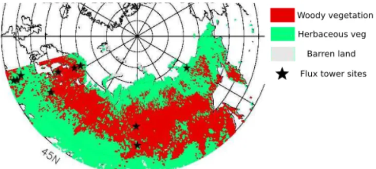
Environmental controls on the increasing GPP of terrestrial vegetation across northern Eurasia
Texto
Imagem
Documentos relacionados
Na hepatite B, as enzimas hepáticas têm valores menores tanto para quem toma quanto para os que não tomam café comparados ao vírus C, porém os dados foram estatisticamente
É nesta mudança, abruptamente solicitada e muitas das vezes legislada, que nos vão impondo, neste contexto de sociedades sem emprego; a ordem para a flexibilização como
didático e resolva as listas de exercícios (disponíveis no Classroom) referentes às obras de Carlos Drummond de Andrade, João Guimarães Rosa, Machado de Assis,
Dentro destes grupos de seres vivos, e em muitas referências, diversos autores referem que as carnes fermentadas podem conter, durante o processamento e no produto final,
Este modelo permite avaliar a empresa como um todo e não apenas o seu valor para o acionista, considerando todos os cash flows gerados pela empresa e procedendo ao seu desconto,
i) A condutividade da matriz vítrea diminui com o aumento do tempo de tratamento térmico (Fig.. 241 pequena quantidade de cristais existentes na amostra já provoca um efeito
Despercebido: não visto, não notado, não observado, ignorado.. Não me passou despercebido
In practice, it reaffirmed ICANN‘s responsibilities regarding a set of goals established in the beginning, the most important being the effort to establish
