The GRAPE aerosol retrieval algorithm

(1)

AMTD

2, 981–1026, 2009

GRAPE aerosol retrieval algorithm

G. E. Thomas et al.

Title Page Abstract Introduction Conclusions References

Tables Figures

◭ ◮

Back Close

Full Screen / Esc

Printer-friendly Version Interactive Discussion

Atmos. Meas. Tech. Discuss., 2, 981–1026, 2009 www.atmos-meas-tech-discuss.net/2/981/2009/ © Author(s) 2009. This work is distributed under the Creative Commons Attribution 3.0 License.

Atmospheric Measurement Techniques Discussions

Atmospheric Measurement Techniques Discussionsis the access reviewed discussion forum ofAtmospheric Measurement Techniques

The GRAPE aerosol retrieval algorithm

G. E. Thomas1, C. A. Poulsen2, A. M. Sayer1, S. H. Marsh1,*, S. M. Dean1,**,

E. Carboni1, R. Siddans2, R. G. Grainger1, and B. N. Lawrence2

1

Atmospheric, Oceanic and Planetary Physics, University of Oxford, Oxford, UK 2

Space Science and Technology Department, Rutherford Appleton Laboratory, Chilton, Didcot, UK

*

now at: Department of Medical Physics and Bioengineering, Christchurch Hospital, New Zealand

**

now at: National Institute of Water and Atmospheric Research, Wellington, New Zealand Received: 12 March 2009 – Accepted: 19 March 2009 – Published: 8 April 2009

Correspondence to: G. E. Thomas (gthomas@atm.ox.ac.uk)

(2)

AMTD

2, 981–1026, 2009

G. E. Thomas et al.

Tables Figures

◭ ◮

Back Close

Full Screen / Esc

Abstract

The aerosol component of the Oxford-Rutherford Aerosol and Cloud (ORAC) combined cloud and aerosol retrieval scheme is described and the theoretical performance of the algorithm is analysed. ORAC is an optimal estimation retrieval scheme for deriving cloud and aerosol properties from measurements made by imaging satellite

radiome-5

ters and, when applied to cloud free radiances, provides estimates of aerosol optical depth at a wavelength of 550 nm, aerosol effective radius and surface reflectance at 550 nm. The aerosol retrieval component of ORAC has several incarnations – this pa-per addresses the version which opa-perates in conjunction with the cloud retrieval com-ponent of ORAC (described by Watts et al., 1998), as applied in producing the Global

10

Retrieval of ATSR Cloud Parameters and Evaluation (GRAPE) data-set.

The algorithm is described in detail and its performance examined. This includes a discussion of errors resulting from the formulation of the forward model, sensitivity of the retrieval to the measurements anda priori constraints, and errors resulting from assumptions made about the atmospheric/surface state.

15

1 Introduction

Despite the important role that atmospheric aerosols play in both climate forcing (both direct and through their interactions with clouds) (IPCC, 2007; Lohmann and Feichter, 2005) and air quality, there are relatively few long term data sets showing their spatial distribution and evolution through time. Imaging satellite instruments o_ffer the ability to

20

provide such measurements and many algorithms have been developed to exploit this ability for specific instruments (Veefkind and de Leeuw, 1998; Mishchenko et al., 1999; Martonchik et al., 1998, 2002; von Hoyningen-Huene et al., 2003; Remer et al., 2005; Grey et al., 2006). In this paper an optimal estimation algorithm for the retrieval of aerosol loading from space-borne visible/near-infrared radiometers, is described and

25

(3)

AMTD

2, 981–1026, 2009

G. E. Thomas et al.

Tables Figures

◭ ◮

Back Close

Full Screen / Esc

measurements from the Along Track Scanning Radiometer 2 (ATSR-2) is given. The ORAC algorithm makes use of a numerical retrieval scheme to fit modelled ra-diances across a series of wavelength bands (channels) to rara-diances measured by a satellite instrument, as a function of aerosol optical depth, effective radius and surface reflectance. The algorithm was developed from the Enhanced Cloud Processor (ECP)

5

(Watts et al., 1998) and the version described here is part of a unified cloud and aerosol algorithm. This algorithm uses a empirical cloud flagging scheme to differentiate cloud and aerosol pixels. Pixels identified as cloud have the cloud retrieval algorithm applied, with the remaining pixels having the aerosol retrieval applied. The algorithm has been applied to ATSR-2, Advanced-ATSR and Spinning Enhanced Visible-InfraRed Imager

10

(SEVIRI) data (Kokhanovsky et al., 2007; Thomas et al., 2007b), including the creation of the GRAPE global cloud and aerosol data-set derived from the full ATSR-2 data-set, spanning 1995–20011. For descriptions of the ATSR-2, AATSR and SEVIRI instru-ments the reader is referred to Mutlow et al. (1999), Llewellyn-Jones et al. (2001) and Aminou et al. (1997), respectively.

15

The ORAC aerosol retrieval algorithm described here is one of three distinct versions of the algorithm, the other two being more advanced stand alone aerosol retrievals. This version of the algorithm was designed as an extention to the existing cloud re-trieval and as such uses a relatively simple forward model, particularly in its treatment of the surface reflectance, which (in common with the cloud retrieval) is treated as

20

Lambertian. This results in important limitations to the algorithm:

– The algorithm is only applicable over surfaces which can be reasonably approx-imated by a Lambertian reflectance, such as the ocean surface far from the sunglint region, and homogeneous land surfaces.

– The use of a Lambertian surface reflectance prohibits the inclusion of near

simul-25

1

(4)

AMTD

2, 981–1026, 2009

G. E. Thomas et al.

Tables Figures

◭ ◮

Back Close

Full Screen / Esc

taneous observations of the same scene at different viewing geometries, such as o_ffered by the ATSR instruments’ dual-view system. Even if a surface can be ap-proximated with an effective Lambertain reflectance for a given viewing geometry, this value can be different for different viewing geometries.

– In the case of instruments such as ATSR-2 and SEVIRI, which have a small

num-5

ber of channels in the visible and near-infrared, the retrieval becomes highly de-pendant on gooda priori knowledge of the surface reflectance. This is because the measurements do not contain enough information to decouple the surface and atmospheric components of the signal.

Despite these limitations, the GRAPE dataset has shown that the algorithm can provide

10

aerosol properties of suffient accuracy to be scientifically interesting, particularly over the open ocean. This is particularly true, since the GRAPE dataset covers a time period prior to the launch of MODIS and MISR. A detailed validation and characterisation of the GRAPE aerosol dataset itself will be presented in a forthcoming paper. For an overview of all versions of the ORAC aerosol algorithm, including a multiview algorithm

15

that makes use of a BRDF description of the surface reflectance, the reader is referred to Thomas et al. (2009).

In Sect. 2 the ORAC forward model and numerical retrieval scheme are described. Section 3 is devoted to a discussion of the algorithm’s performance and limitations, including the sensitivity of the algorithm and investigation of sources of error. The

20

results are summarised and conclusions drawn from them are given in Sect. 4.

2 Forward model and retrieval algorithm

2.1 The forward model

The ORAC aerosol forward model can be thought of as being composed of four com-ponents:

(5)

AMTD

2, 981–1026, 2009

G. E. Thomas et al.

Tables Figures

◭ ◮

Back Close

Full Screen / Esc

1. A model of aerosol radiative properties (single scatter albedo, extinction coeffi -cient and phase function) at the required wavelengths as a function of aerosol size distribution and spectral refractive indices. Ideally the aerosol radiative properties should be computed across the channel bandpass functions of the instrument in question, but for most radiometers the width of each channel is small compared

5

to the scale over which the aerosol radiative properties vary and thus the compu-tation can be done for the weighted centre wavelength of each channel.

2. A model of gas absorption (or emission) over the bandpass of each channel. 3. A model or measurements of the surface reflectance, both of the land and ocean. 4. A radiative transfer model, which predicts the top of atmosphere radiance as a

10

function of the radiative properties produced by the aerosol and gas models, the surface reflectance, and illumination and viewing angle.

For reasons of numerical efficiency, radiative transfer calculations are done off-line for a range of aerosol properties and viewing geometries to produce look-up tables, which are then used to predict the radiance during retrieval runs.

15

ORAC uses Mie scattering to relate aerosol microphysical properties to their radia-tive properties. It should be noted that Mie scattering is only applicable to spheri-cal particles and thus its use will introduce errors in the radiative properties of non-spherical aerosol particles (the most notable example being mineral dust). Although not included in this analysis, the development of non-spherical scattering code for use

20

with the ORAC scheme is underway.

Microphysical properties are taken from published descriptions of typical atmo-spheric aerosol types, such as those found in the Optical Properties of Aerosols and Clouds (OPAC) database (Hess et al., 1998). Such models typically describe a range of atmospheric aerosol classes, each of which is made up of an external mixture of

25

(6)

AMTD

2, 981–1026, 2009

G. E. Thomas et al.

Tables Figures

◭ ◮

Back Close

Full Screen / Esc

its own size distribution. For use with ORAC, each component is assumed to have a log-normal size distribution

n(r)= _√N0

2π 1 lnS

1 r exp

"

−(lnr −lnrm)

2

2 ln2S

#

(1)

where the median radiusr_m and spreadS (where the standard deviation of lnr is lnS) are taken from the aerosol database.

5

Mie scattering theory is then used to produce the single scatter albedo (ωi), extinc-tion coefficient (β_iext) and phase function (p_i) of each component, i, from which the values for the complete aerosol class can be calculated using:

β_ext₌ Σiχiβ

ext

i

Σiχi

(2)

ω₌ Σiχiβ

ext

i ωi

Σiχiβexti

(3)

10

p₌ Σiχiβ

ext

i ωipi

Σiχiβ_iextωi

(4)

whereχ_i is the mixing ratio of theith component.

To enable the retrieval of aerosol size information, these quantities must be calcu-lated for a range of different aerosol size distributions. The measure of the aerosol size used by ORAC is the effective radius, which is defined as the ratio of the third and

15

second moments of the aerosol size distribution. For a log normal distribution this is

r_e₌ Σiχir

3

m,iexp(4.5 ln

2

S_i)

Σiχirm,i2 exp(2 ln

2_S

i)

(7)

AMTD

2, 981–1026, 2009

G. E. Thomas et al.

Tables Figures

◭ ◮

Back Close

Full Screen / Esc

Each aerosol class will have a prescribed r_e (defined by the r_m and χ of each com-ponent). Optical properties are produced for a range of e_ffective radii by changing the mixing ratios of the components. If an r_e is desired that is either smaller than that of the smallest component, or larger than that of the largest component, the aerosol class becomes a single component aerosol (since the r_e will have been minimised,

5

or maximised, by setting the mixing ratio of the appropriate component to 100%). In such a case, the desired r_e is achieved by scaling the median radius of the one re-maining component. It is obvious that by changing the e_ffective radius in this fashion, the aerosol class will quickly lose its resemblance (not only in terms of size, but com-position) to its source class as defined by the literature. Thus, ORAC works on the

10

implicit assumption that oura priori knowledge of the aerosol we expect to observe is reasonably accurate, so that large changes to the effective radius are not needed to match the observed radiances.

The modelling of gas absorption or emission over the wavelength bands of the in-strument is performed using MODTRAN (Berk et al., 1998). As the retrieval uses

15

visible/near-infrared wavelengths, the signal from atmospheric gases is dominated by Rayleigh scattering rather than absorption/emission. Thus temporal and spatial variation in the gas composition of the atmosphere can be neglected and standard-atmosphere gas concentrations can be used2. The modelled gas absorption is then convolved with the instrument filter function at each channel to produce an optical depth

20

due to gas absorption/emission.

Both the aerosol radiative properties and the gas optical depth are then passed to the DISORT (Stamnes et al., 1988) radiative transfer code, which models the radiance for each combination of aerosol effective radius and optical depth (determined by the number density of aerosol) over the plausible range of illumination and viewing angles

25

2

(8)

AMTD

2, 981–1026, 2009

G. E. Thomas et al.

Tables Figures

◭ ◮

Back Close

Full Screen / Esc

for the given satellite. A 32 layer model of the atmosphere, extending to a height of 100 km is used for the DISORT calculations. In layers containing aerosol, the e_ffects of molecular absorption, Rayleigh scattering and aerosol scattering and absorption are combined using the following expressions:

τ_l₌τ_a₊τ_R₊τ_g (6)

5

ω_l₌ τR +τaωa

τ_a₊τ_R₊τ_g (7)

p_l₌ τRpR+τaωapa

τ_R₊τ_aω_a (8)

whereτ_a,τ_R,τ_g are the optical depths due to aerosol, Rayleigh scattering and molec-ular absorption within the layer, which combine to give a total optical depth of τ_l for the layer. The single scattering albedo for each layer,ω_laverage single scatter albedo

10

of the aerosol, Rayleigh scattering (for whichω_R_≡1) and molecular absorption (where ω_g_≡0), weighted by their optical depths. Likewise, the phase function for each layer is also a weighted mean, with weights being the fraction of the optical depth for each process which is due to scattering (i.e.τω). All of these calculations are performed as-suming a black surface and assume a constant illumination, producing a set of effective

15

transmissions and reflectances for di_ffuse and direct-beam radiation for the atmosphere as a whole.

This allows radiative transfer through the Earth’s atmosphere to be treated as a series of partial reflections and transmissions. The first of these is a “reflection” of the solar beam off the atmosphere itself, described by a bidirectional reflectance

20

R_bb(θ0, θv, φ), as a function of solar and viewing zenith angles,θ0andθvand the

rela-tive azimuth angleφ. The subscript bb indicates that this reflectance function takes a direct-beam input and provides a direct-beam output. This is followed by a term com-posed of the transmission of the solar beam through the atmosphere (T_bt↓(θ0), where bt

indicates the transmission function accepts a direct beam as input and produces both

(9)

AMTD

2, 981–1026, 2009

G. E. Thomas et al.

Tables Figures

◭ ◮

Back Close

Full Screen / Esc

beam and diffusely transmitted components), reflection offa Lambertian surface with reflectanceρ and transmission of the resulting di_ffuse radiation back through the at-mosphere (T_tb↑(θv)) to the satellite. Subsequent terms result from multiple reflectances

between the surface and the atmosphere (described by a diffuse reflectanceR_dd). The resulting geometric series:

5

R₌R_bb(θ0, θv, φ)+T_bt↓(θ0)ρT_tb↑(θv) +T_bt↓(θ₀)ρ2T_tb↑(θ_v)R_dd

+T_bt↓(θ0)ρ3T_tb↑(θv)R_dd2

+... (9)

can be simplified using the appropriate series limit to give

10

R₌R_bb(θ0, θv, φ)+

T_bt↓(θ₀)ρT_tb↑(θ_v)

1−ρR_dd . (10)

Lookup tables of the quantitiesR_bb(θ0, θv, φ), T_bt↓(θ0), T_tb↑(θv), and Rdd are created by

DISORT as a function of aerosol optical depth, effective radius, solar zenith angle, satellite zenith angle and relative azimuth angle (as appropriate).

The final aspect of the forward model is a description of the reflectance of the Earth’s

15

surface across each of the desired channels. ORAC retrieves the surface albedo at 0.55µm but the spectral shape (i.e. the ratio of the albedo at each channel to 0.55µm) is fixed by the a priori spectral albedo. The determination of the a priori albedo, is treated separately for land and ocean pixels. Over land the MOD43B Bi-directional Reflectance Distribution Function (BRDF) product from MODIS (Jin et al., 2003) is

20

(10)

AMTD

2, 981–1026, 2009

G. E. Thomas et al.

Tables Figures

◭ ◮

Back Close

Full Screen / Esc

2.2 Retrieval algorithm

ORAC is an optimal estimation retrieval scheme, based on the formalism of Rodgers (2000). It uses a numerical minimisation to determine the maximuma posterisolution, that is the solution that has the maximum probability of being the “truth” according to Bayesian statistics, to the problem of matching the observed and modelled radiances.

5

This solution is given by minimising, via an iterative optimisation, the cost function: J(x)=(Y₋F(x))TS−_ǫ1(Y₋F(x))+(x₋x_a)TS_a−1(x₋x_a) (11) where Y is the vector of measured radiances, F(x) is the corresponding forward-modelled radiances andSǫ is the measurement covariance matrix, which defines the uncertainty of each measurement and the correlations between them. xis the vector

10

of state variables (i.e. the values we are retrieving), with the a priori state vector x_a

and corresponding covariance matrixSa, defining our knowledge of the state before the measurement and the uncertainty in this knowledge, respectively. The state vector for the ORAC retrieval is made up of the aerosol optical depth at 550 nm, the aerosol effective radius and the surface reflectance at 550 nm:

15

x=

 

τ_a r_e ρ(550)



. (12)

The inclusion of prior knowledge of the state in a rigorous way is a particular strength of the optimal estimation approach. The retrieval can be viewed as a process of us-ing the measurements to better define our prior knowledge of the state, whether that knowledge be based on a climatology or on independent measurements of the state.

20

The other advantage of the optimal estimation framework over other, more ad hoc, retrieval methods is that it provides information on the quality of the retrieval. The first indicator of a successful retrieval is that it has converged. Successive iterations each produce their own estimate of the state and when the difference between these estimates becomes a small fraction of their estimated precision, the retrieval can be

(11)

AMTD

2, 981–1026, 2009

G. E. Thomas et al.

Tables Figures

◭ ◮

Back Close

Full Screen / Esc

said to have converged. In practice, an upper limit is put on the number of iterations the retrieval can take (in the case of ORAC this is set to 25): if a retrieval has not converged within this number of steps, it is deemed to have failed. In addition, the value of the cost function at the final solution and error estimates on the retrieved state provide indicators as to the quality of the retrieval. The former indicates how consistent

5

the solution is with the measurement anda priori information, while the latter defines how well constrained the solution is.

To calculate uncertainties on the retrieved state, the assumption is made that for small changes in the state vector the forward model can be considered linear, so that it can be expressed as

10

F(x)−F(ˆx)=Kˆ(x−ˆx). (13)

Here ˆx and K are the state vector and weighting function matrix at the solution.The weighting function matrix contains the derivatives of the forward model with respect to the state vector:

K_{i j} ₌ ∂Fi(x)

∂x_j , (14)

15

where thei andj subscripts denote elements of the measurements and state vectors respectively. Under this assumption, we can relate the covariance of the measure-ments anda priori state to the uncertainty in the retrieved stateSˆ via,

ˆ

S=KˆTS−_ǫ1Kˆ +S−_a1−1. (15)

ORAC uses the Levenburg-Marquardt algorithm (Levenberg, 1944; Marquardt, 1963)

20

to perform the minimisation of the cost function. This provides an extremely robust and numerically efficient method for minimisation which will converge successfully even for highly non-linear problems. However it has no mechanism to avoid becoming trapped in local minima in the cost function. Furthermore, if the forward model is highly non-linear in the region surrounding the solution, the optimal estimation error propagation

25

(12)

AMTD

2, 981–1026, 2009

G. E. Thomas et al.

Tables Figures

◭ ◮

Back Close

Full Screen / Esc

3 Retrieval performance

In this section we examine the theoretical performance of the ORAC aerosol retrieval algorithm in the configuration used in the GRAPE project, using the results of retrieval runs on simulated data that resembles measurements made by the ATSR-2 (or AATSR) instrument. Two questions are addressed:

5

1. How sensitive is the retrieval to changes in the state parameters? This gives us a measure of the best possible precision and accuracy we can expect the retrieval scheme to achieve, given the measurements we are providing.

2. How sensitive is the retrieval to errors in the forward model and assumptions made about aerosol and surface properties.

10

The configuration of the ORAC processor used in the GRAPE project uses channels 2–4 of the ATSR-2 instrument (centred on wavelengths of 0.67, 0.87 and 1.6µm). The 0.55µm channel is not used, as over the oceans it is either disabled, or in a narrow-swath(where the swath width of the instrument is reduced from 512 to 256 km), due to down-link bandwidth limitations of the ERS-2 satellite. The retrieval assumes an

15

aerosol type based on the geographic location of each pixel and time of year, as shown in Fig. 1, with the possible types being maritime clean, continental average, desert dust, Arctic and Antarctic classes from the OPAC database.

Measurement uncertainties are set at fixed values of 0.005, 0.009, and 0.018 for channels 2, 3 and 4. These values were determined for cloud retrievals and are slight

20

over-estimates of the noise expected on ATSR-2 measurements for the lower radiances typical of aerosol measurements. However, given the forward model errors discussed below, these values are considered appropriate. Additional error to account for both the Lambertian surface reflectance approximation and the constraint of a fixed spectral shape to the surface reflectance is also included inSǫ at 20% of the a priori surface

25

(13)

AMTD

2, 981–1026, 2009

G. E. Thomas et al.

Tables Figures

◭ ◮

Back Close

Full Screen / Esc

The aerosol optical depth and effective radius are retrieved in log10 space, while the

surface reflectance is retrieved on a linear scale. Thea priori and first guess surface albedo are set to the value defined by the sea-surface reflectance model over the ocean or the MODIS white-sky albedo over the land, with a 1σerror of 0.01. Thea priori and first guess values for optical depth are set to log₁₀(τ)₌₋1.0_±1.0, corresponding to

5

τ₌0.1 with 1σerror bounds of 0.01≤τ_≤1.0. Thea priori and first guess effective radius is set to the value prescribed in literature for each aerosol type, with error bounds of

±0.5 in log₁₀(r_e).

3.1 Retrieval sensitivity

The foremost limitation on the performance of a retrieval system is the information

con-10

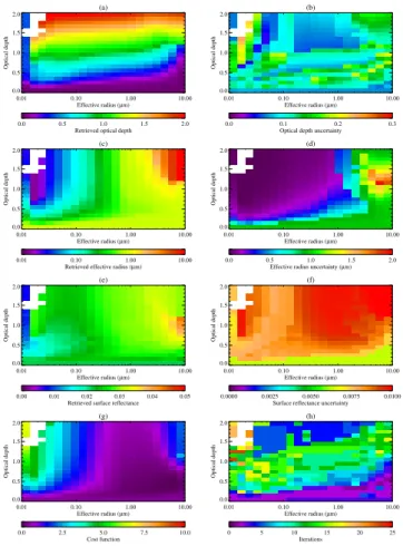
tent of the measurements themselves and how sensitive each retrieved parameter is to perturbations in the state. This limitation can be investigated by performing the retrieval on simulated data, so that all sources of forward model and forward model parameter error can be removed from the problem. Figure 2 shows the aerosol state parameters (optical depth and e_ffective radius) which have been used to produce simulated ATSR-2

15

radiances using the optical properties of the OPAC maritime clean aerosol class. The retrieval has been run on these data, assuming the correct aerosol class and with thea priorisurface reflectance set to the correct value. The a priori e_ffective radius for the maritime clean class is 0.832µm, giving 1σ error bounds of 0.26<re<2.63µm. The results of applying the retrieval to these data are given in Fig. 3, along with error

20

estimates derived from the diagonal of the state covariance matrix, the value of the cost function at the solution and the number of iterations required for convergence. The first thing to notice is that some retrievals have failed to converge at the lowest effective radius (as indicated by white spaces in Fig. 3). This can be attributed to the optical depth being poorly constrained for the lowest size bin, as indicated by the

25

(14)

AMTD

2, 981–1026, 2009

G. E. Thomas et al.

Tables Figures

◭ ◮

Back Close

Full Screen / Esc

Figure 3g shows that the cost function at the solution has a value which is always less than 6. The smooth dependence on the state exhibited by the cost function is due to thea priori portion of the cost function ((x−xa)

T

S−a1(x−xa)): i.e. the retrieval is fitting the measurements extremely well for all states, with the cost function being essentially determined by the distance from thea priori. Statistically, one expects the cost function

5

to follow a χ2 distribution with a single degree of freedom3. This is not the case in this example, because the simulated measurements used in the retrieval did not have noise added to them, thus the forward model can consistently fit the measurements more accurately than predicted by the measurement covariance matrix,Sǫ.

It is also very clear that the retrieval has failed to accurately estimate the true fields

10

for states with low optical and large e_ffective radius. To further explore why this is the case, we will examine the retrieval statistics further. Rodgers (2000) defines the averaging kernel for the maximuma posteriori solution as

A=SaKˆT

ˆ

KSaKˆT +Sǫ

−1 ˆ

K. (16)

This matrix gives the sensitivity of the retrieved state to perturbations in the true state,

15

A_{i j} ₌ ∂xˆj

∂x_i, (17)

where ˆx_j is thejth element of the retrieved state andx_i is theith element of the true state. The diagonal elements of this matrix can be thought of as an indication of the fraction of the retrieved state which can be said to be determined by the true value of that quantity (with the rest being determined by the choice ofa priori and the value of

20

the other elements of the state). For a perfect retrieval systemAwould be an identity matrix, while a value of zero on the diagonal indicates that the corresponding state element is entirely determined by thea priori and values of the other state elements.

3

(15)

AMTD

2, 981–1026, 2009

G. E. Thomas et al.

Tables Figures

◭ ◮

Back Close

Full Screen / Esc

The trace of the averaging kernel also gives the degrees of freedom for signal for the given retrieval. This quantity gives the number of pieces of independent information retrieved. It is important to realise thatd_s is not a direct estimate of the information content of the measurement, but rather indicates how much the measurement is able to improve our prior knowledge of the state. Figure 4 shows the diagonal elements of

5

A, as well the overalld_s corresponding to the retrieval shown in Fig. 3. The first thing to note is thatd_s.2.5, indicating that the retrieved state is always somewhat influenced by thea priori. Looking at Fig. 4a–c, we can see that in general optical depth is most sensitive to the measurement, as is effective radius at large optical depths, whereas the surface reflectance is mostly dominated by thea priori value.

10

It can also be seen that the regions of the domain where the retrieval has done least well (in particular, where optical depth is low and effective radius high) correspond to regions whered_sis low and the effective radius shows poor sensitivity to the true state. In such circumstances the e_ffective radius is held at thea priori value and this results in an error in the retrieved optical depth, despite its good sensitivity to the true state.

15

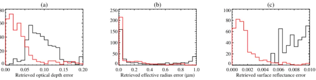
Figure 5 shows the distribution of retrieved error estimates for each of the state el-ements, along with the distribution of the difference between the retrieved and true states. It can be seen that most retrievals provide optical depth to a precision between 0.05 and 0.15, while the majority of effective radii have a precision of less than 0.1. It is clear that for most states, the retrieved optical depth is more accurate than indicated

20

by the retrieved error estimate. As with the low values of the cost function shown in Fig. 3g, this can be explained by the fact that no measurement noise was added to the simulated radiances used in the retrieval. The retrieved error estimates give the 1σ confidence interval on the retrieved values, given the measurement anda priori uncer-tainties: since the simulated measurements actually contain no error, the accuracy of

25

the retrieval is substantially better than this estimate4.

The surface reflectance error distribution shows somewhat different behaviour, since 4

(16)

AMTD

2, 981–1026, 2009

G. E. Thomas et al.

Tables Figures

◭ ◮

Back Close

Full Screen / Esc

the retrieval used the correct value for the first guess and a priori. In addition, the surface reflectance is retrieved on a linear scale, while the log₁₀ of optical depth and effective radius are retrieved. Thus the maximum of the retrieved surface reflectance error distribution is defined by the a priori error (while the retrieved error for optical depth and e_ffective radius depends on the value of the retrieved state and hence has

5

a relative, rather than an absolute, maximum). It is clear from Fig. 5c that the retrieval has somewhat narrowed the confidence interval on the value of surface reflectance for many states, but many more have not been improved at all.

Taken together, Figs. 3, 4 and 5 tell us several things about the retrieval:

– Overall, the retrieval is working well as there is an improvement in our knowledge

10

of almost all states (given by the narrowing of the uncertainties from theira priori values) and the retrieved states almost always agree with the true value within uncertainty estimates.

– The retrieval works best a high optical depths or effective radii between approxi-mately 0.015 and 0.10.

15

– Where the retrieval is working well, optical depth and effective radius are both retrieved with a precision of.0.1.

– The measurement is adding between 1 and approximately 2.5 independent pieces of information to the system at this level of a priori constraint – i.e. the retrieval is under-constrained, since we are attempting to retrieve more quantities than we

20

have pieces of information from the measurement.

– Surface reflectance is poorly retrieved, with the a priori accounting for 50% or more of the retrieved value. Optical depth and effective radius show good sensi-tivity to the true state throughout most of the range.

– The strange feature in the effective radius fields above a true effective radius of

25

(17)

AMTD

2, 981–1026, 2009

G. E. Thomas et al.

Tables Figures

◭ ◮

Back Close

Full Screen / Esc

where effective radius is poorly constrained by the measurements. Correspond-ing patterns in the surface reflectance fields indicate some degeneracy between these two variables. It is also notable that the optical depth retrieval remains quite stable throughout this region of state space.

The accuracy of the a priori surface reflectance also has a strong influence on the

5

accuracy of the retrieved parameters. Although ORAC retrieves the magnitude of the surface reflectance, it is tightly constrained to thea priori. This constraint is required because of the limited amount of information available in the measurements – if the surface reflectance is not tightly constrained, the retrieval is prone to converging on highly unrealistic states: i.e. the cost function has multiple minima. The effect of a 0.01

10

error (i.e. equal to the a priori error) in the first guess and a priori value of surface reflectance is shown in Fig. 6. In terms of the retrieval of optical depth and effective radius these results are strikingly similar to those shown in Fig. 3, and it is evident that the retrieval has moved the surface reflectance towards the correct value from the a priori. The uncertainty estimates on the retrieved states are also similar to those

15

shown in Fig. 3, as are the cost function and iterations, showing that the retrieval is able to fit the measurements as well and as quickly as when the correcta priorisurface reflectance is used.

Figure 7 shows the results of increasing the first guess and a priori surface re-flectances to 0.05. In this case it is clear that the retrieval is unable to compensate

20

for the larger discrepancy, particularly at either large, or the smallest effective radii, where the retrieved state is grossly different to the truth and the retrieved surface has not moved from thea priori value. The retrieved uncertainty estimates are again sim-ilar to those in Fig. 3. Unsurprisingly, the retrieval deals with an error in the assumed surface reflectance better when the aerosol optical depth is high, as in this case the

25

(18)

re-AMTD

2, 981–1026, 2009

G. E. Thomas et al.

Tables Figures

◭ ◮

Back Close

Full Screen / Esc

trieval system: the effect of the incorrect surface reflectance can be compensated for by changes in optical depth and e_ffective radius.

These results indicate that the retrieval is able to compensate for errors in the a priori surface reflectance of the order of the a priori error, but not much larger than this. Unfortunately the retrieved state is still consistent with the measurements anda

5

priori(as indicated by very similar retrieval costs) in both of these cases, meaning that it would not be possible to detect instances of poor a priori surface characterisation from the retrieval itself5.

3.2 Forward model errors

The term forward model error refers to inaccuracies that result from incomplete or

10

incorrect modelling of the relevant physical processes by the forward model. In the case of ORAC, these can be divided into four main categories:

1. Errors in modelling the scattering from the aerosol itself; in particular, from the assumption of sphericity implicit in the use of Mie scattering.

2. Errors resulting in the discrete ordinates radiative transfer approach, including the

15

assumption that the surface acts as a Lambertian reflector.

3. Assumptions made in the formulation of the forward model expression (Eq. 10) used in the retrieval.

4. Interpolation errors due to the use of discrete look-up tables for the transmission and reflectance terms in Eq. 10.

20

5

(19)

AMTD

2, 981–1026, 2009

G. E. Thomas et al.

Tables Figures

◭ ◮

Back Close

Full Screen / Esc

As mentioned in Sect. 2, the first of these sources of error is not addressed in this paper, although work is ongoing to investigate its effects and incorporate non-spherical scattering into the ORAC system. The modelling of atmospheric gas absorption, emis-sion and Rayleigh scattering is another potential source of error, but the authors are confident that this is a minor contribution, particularly in the case of the ATSR

instru-5

ments and SEVIRI, where the radiance error due to the assumptions made in the forward model is significantly smaller than the random error on the measurements. It should be noted that forward model error is unavoidable, especially if the retrieval algo-rithm is to be reasonably computationally efficient. As long as the sum of the forward model errors are kept well below the measurement noise level, however, their effects

10

will be minimal.

The error due to the DISORT radiative transfer will be dominated by the Lamber-tian surface reflectance approximation, except at high zenith angles (>75◦) where the plane-parallel assumption of DISORT breaks down. This is a well known limitation of the DISORT method and is avoided by only running the retrieval on data which

15

meets the plane parallel criterion. In order to investigate the effect of the Lamber-tian surface approximation, DISORT was used to model TOA reflectances (following a similar procedure to the calculation of the look-up tables) for both a bi-directional sur-face reflectance and an equivalent Lambertian reflectance. The MODIS BRDF product was used to provide a variety of surface reflectances which span the typical range

20

for land surfaces (the ocean surface reflectance has been neglected in this analysis, but it is generally far more isotropic than land surfaces, except for areas effected by strong sun-glint). The calculation was repeated for a wide range of viewing geometries, aerosol loading and surfaces ranging from desert to dense forest. Results show that the Lambertian approximation generally over-estimates the directional surface reflectance

25

(20)

AMTD

2, 981–1026, 2009

G. E. Thomas et al.

Tables Figures

◭ ◮

Back Close

Full Screen / Esc

of the BRDF for all viewing geometries.

The latter two of the error terms listed at the begining of this section can be quantified by comparing TOA reflectances computed directly from DISORT to those computed us-ing the look-up tables and the forward model equation. Point 3 can be investigated by comparing the two qualities for viewing geometries and aerosol properties which

cor-5

respond to points in the look-up tables (so that no interpolation is required). Point 4 can then be examined by doing the comparison for values which lie half-way between the look-up table points (where interpolation errors can be expected to be maximum). This procedure has been followed for 4500 points across a wide range of viewing ge-ometries and particle states, as summarised in Table 1.

10

For values coincident with the look-up table points the forward model and DISORT agree to within±0.2% for most viewing geometry and aerosol loading combinations, and always agreeing to within±0.6%. There is, on average, a small positive bias ap-parent in the forward model expression, with the mean di_fference being 0.14% (median 0.14%). However, it is clear that for a Lambertian surface, Eq. (10) reproduces the

15

DISORT modelled TOA radiances well.

Comparisons made for values where the effects of look-up table interpolation are maximised show that the interpolation error can far out-weigh that from the approxima-tions made in Eq. (10). In some instances, it is possible for interpolation to introduce over 5% error into the modelled radiances, although for the vast majority of viewing

20

angle/aerosol loading combinations the discrepancy is much lower than this. For this worst case ensemble of points the mean difference between the forward model and DISORT is₋0.99% (median₋0.72%).

Smith et al. (2002) quotes errors on ATSR-2 visible/near-infrared radiances as being approximately 2%, based on the accuracy of the on-board calibration system. Hence

25

(21)

AMTD

2, 981–1026, 2009

G. E. Thomas et al.

Tables Figures

◭ ◮

Back Close

Full Screen / Esc

3.3 Forward model parameter error

Forward model parameter errorresults from uncertainties in the parameters used in the computation of the forward model that are not included in the retrieval process. There are two main inputs into the modelled radiances which are most likely to significantly affect the output radiances:

5

1. The aerosol properties used in the calculation of the look-up tables (including the assumed size distribution, refractive indices and vertical distribution of the aerosol).

2. The spectral dependence of the surface reflectance.

In this section the effects on the retrieval of errors in a range of forward model

pa-10

rameters will be examined with a series of retrievals on simulated data, similar to that presented in Sect. 3.1. The effects to be examined are:

1. The effect of using an inappropriate aerosol calss. The ORAC retrieval does not include any ability to retrieve the composition of aerosol (aside from that implied by the change in composition that accompanies a change in effective radius) –

15

it relies entirely on the accuracy of assumed optical properties, such as those provided by the OPAC database.

2. The effect of incorrect assumptions about the aerosol size distribution. Although the aerosol e_ffective radius is retrieved, the form of the size distribution is fixed (to that defined in the OPAC database, for example).

20

3. The vertical distribution of aerosol used is an assumed, fixed profile. One might assume that the TOA radiance in the visible is largely insensitive to the height distribution of aerosol, but this should be quantified.

4. The effect of incorrect assumptions about the spectral dependence of the surface reflectance. Although ORAC is able to retrieve surface reflectance to a limited

(22)

AMTD

2, 981–1026, 2009

G. E. Thomas et al.

Tables Figures

◭ ◮

Back Close

Full Screen / Esc

gree, it is only its magnitude which is permitted to vary. The spectral dependence is fixed at thea priori value.

Errors in any of these parameters will result in inaccuracies in the retrieved aerosol parameters. However, due to the non-linearity and complexity of the effects, and lack of knowledge about the accuracy of any one of them for a given retrieval, it is not practical

5

to attempt to characterise them with standard Gaussian error statistics. Indeed it is not even meaningful to attempt to define “typical” values for such errors, since their effects are likely to be so variable. Thus, the approach taken here is to test the retrieval in situations where the sources of error are completely known, in order to provide indications of the magnitudes of each effect.

10

3.3.1 Incorrect aerosol properties

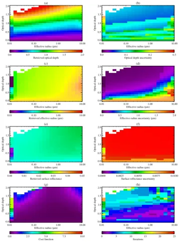
Figure 8 shows retrieval results when ORAC is applied to simulated radiances pro-duced using the maritime-clean aerosol class from the states shown in Fig. 2, but using the OPAC desert dust aerosol class in the retrieval. It is encouraging to see that the optical depth field still shows a reasonable agreement with the input field. Overall

15

however, differences between the true and retrieved fields are much greater than when the correct aerosol properties are used in the the retrieval, particularly in effective ra-dius. What is more, the retrieved uncertainties suggest a higher degree of confidence in the retrieved values than was the case with the correct aerosol class, with the un-certainties on optical depth in particular being much smaller than in Fig. 3. Although

20

this may seem a counter-intuitive result, it must be remembered that it simply indicates that the radiance shows a stronger dependence on aerosol optical depth for the desert aerosol class than for the maritime clean one.

Overall the effect of assuming desert aerosol in place of maritime can be summarised as resulting in dramatic errors in retrieved e_ffective radius, while the optical depth shows

25

(23)

AMTD

2, 981–1026, 2009

G. E. Thomas et al.

Tables Figures

◭ ◮

Back Close

Full Screen / Esc

is appropriate – the retrieval has converged to reasonable values, with low costs, for the majority of the states tested. One might expect that if the aerosol optical properties assumed within the retrieval are incorrect, the forward model would not be able to provide a good fit to the measurements, resulting in the cost function having a higher value at the solution. However, there is enough degeneracy in the system to allow

5

incorrect assumptions about the optical properties of the aerosol to lead to a retrieval which is consistent with the measurements anda priori.

If the assumed aerosol properties are very far from the truth however, the retrieval breaks down completely. Figure 9 shows the results of applying the highly absorbing OPAC urban aerosol class to the simulated radiances generated from the

maritime-10

clean class. In this case the retrieval has failed to converge for most high optical depths and those states which have been retrieved have very large uncertainty estimates (on the order of 100% or more). However, even in this case, where the retrieval has con-verged it has done so to a state with a low cost (Fig. 9g) – again demonstrating the high degeneracy of the problem.

15

3.3.2 Aerosol size distribution

The size distribution of an aerosol population can have a great impact on its optical properties, particularly for populations dominated by larger particles. Incorrect assump-tions about the size and number of modes in an aerosol distribution used to model the TOA radiance can thus be expected to have a significant impact on retrieved aerosol

20

properties. To investigate the scale of such errors simulated ATSR-2 radiances were produced in the same way as in Sect. 3.1, but using an aerosol class consisting of a log-normal distribution of sea salt particles (as defined by the accumulation mode sea-salt component defined in OPAC). The retrieval was then run on these data using a bi-modal aerosol class consisting of two log-normal sea-salt distributions (with the

25

(24)

AMTD

2, 981–1026, 2009

G. E. Thomas et al.

Tables Figures

◭ ◮

Back Close

Full Screen / Esc

high optical depth and low effective radius. As might be expected it is the retrieval of e_ffective radius itself which shows the greatest deviation from the truth: the retrieved field has become nearly flat. Again, for much of state space, the retrieved uncertainty estimates for the effective radius give little indication of the inaccuracy of the retrieval. Despite this however, the retrieval of optical depth shows a remarkable robustness:

5

indeed for values less than approximately one, it is as accurate as the retrieval using correct assumptions.

The improvement in the retrieval performance at larger e_ffective radii can be at-tributed to the coarse mode dominating the bi-modal distribution used in the retrieval, which effectively makes this distribution more mono-modal. However, the effective

ra-10

dius retrieval is still poor, and as both the sea-salt modes haves have the same pre-scribed width, this indicates that the retrieved effective radius is very sensitive to the form of the size distribution.

3.3.3 Aerosol height distribution

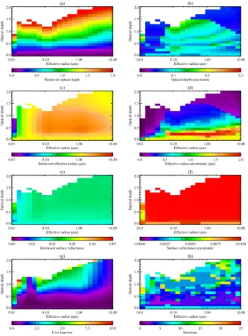
Figures 11 and 12 show two retrievals using the same set of simulated ATSR

radi-15

ances, created with the OPAC desert-dust aerosol class. In calculating the radiances, the aerosol was assumed to lie between 0–2 km (corresponding to the lowest two lev-els of the DISORT forward model), with 60% of the aerosol optical depth lying between 0–1 km. In producing Fig. 11 the retrieval was run with the same assumed height dis-tribution, while for Fig. 12, the aerosol was assumed to lie in a single layer between

20

4–5 km.

The two sets of results show strong similarities, but are not identical, indicating that the retrieval is somewhat sensitive to the height distribution of the aerosol. The ef-fect is most notable at large effective radii, but unlike all the other effects examined in this study, it is the optical depth that shows the greatest perturbation. This is due

25

(25)

so-AMTD

2, 981–1026, 2009

G. E. Thomas et al.

Tables Figures

◭ ◮

Back Close

Full Screen / Esc

lar radiation is scattered towards the surface where, due to the low surface reflectance used in the simulations, it is likely to be absorbed. If the aerosol layer is elevated, there is a layer of Rayleigh scattering between the aerosol layer and the surface. Due to the isotropic nature of Rayleigh scatter, this will effectively increase the reflectance be-low the aerosol and hence produce higher TOA radiances. Thus if the forward model

5

incorrectly makes the assumption of an elevated aerosol layer, it will over-predict the TOA radiance for a given optical depth, resulting in the retrieval under-predicting optical depth to compensate. This will only be noticeable at large aerosol e_ffective radii, be-cause at lower effective radii the aerosol phase function becomes more isotropic. This effect will also depend on viewing geometry, due to the angular dependence of the

10

phase function of large particles. For example, for near-back scattering geometries, tests have shown the effect is not apparent, because the signal is dominated by the strong back scattering peak of the aerosol phase function.

Although the retrieval is not very sensitive to the aerosol height itself, Marsh et al. (2004) shows that the TOA radiance is dependent on the height distribution of aerosol

15

properties. Variation of aerosol properties with height leads to effects similar to those described above, but to a much greater degree. An example analogous to the Rayleigh scattering effect discussed above would be that of a layer of absorbing aerosol over-lying scattering aerosol compared to situation where the two aerosol are mixed in a single layer. In the former case the overlying absorbing layer will absorb a greater

20

proportion of the incoming solar radiation and upwelling radiation scattered from the scattering aerosol below than would be the case if the aerosol were in a mixed layer, thus the TOA radiation will be reduced. The size of this effect will depend strongly on the amount and distribution of each aerosol and is thus difficult to quantify. However, Marsh et al. (2004) shows changes of up to 50% in TOA radiance over dark surfaces

25

(26)

AMTD

2, 981–1026, 2009

G. E. Thomas et al.

Tables Figures

◭ ◮

Back Close

Full Screen / Esc

radius.

It is also interesting to compare Fig. 11 with the other retrieval done using correct assumptions, Fig. 3. The two sets of results show very similar patterns and overall accuracy, which offers some encouragement that the specific results presented in this study are indicative of ORAC retrieval performance in general.

5

3.3.4 Spectral surface reflectance

The final parameter to be examined is the spectral shape of the surface reflectance. This was tested by generating simulated AATSR radiances using the OPAC maritime clean aerosol class with surface reflectances of 0.02, 0.016, 0.012 and 0.008 at 550, 670, 870 and 1600 nm, respectively (i.e. the reflectance has been reduced by 20, 40

10

and 60% from the 550 nm value in the subsequent channels). The retrieval was then applied to the resulting data assuming a spectrally flat surface reflectance of 0.02 in all channels. Figure 13 shows that the retrieved optical depth and effective radius fields are almost as close to the input data as is the case when the retrieval is run with correct assumptions. The retrieved 550 nm surface reflectance shows that the

15

retrieval has produced a lower reflectance at this wavelength in order to compensate for the over-estimate in reflectance at lower wavelengths produced by the assumed flat spectral shape. It should be noted that the sensitivity to thea priori 0.55µm surface reflectance discussed in Sect. 3.1 will limit the ability of the retrieval to deal with very large discrepancies in the surface reflectance spectrum, as the algorithm is unlikely to

20

retrieve a surface reflectance outside the 1σa priori confidence interval.

4 Conclusions

An optimal estimation retrieval of aerosol properties from visible/near-IR satellite im-agery, part of the Oxford-RAL Aerosol and Cloud retrieval scheme (ORAC), has been presented. The algorithm was developed to work within the ORAC cloud retrieval

(27)

AMTD

2, 981–1026, 2009

G. E. Thomas et al.

Tables Figures

◭ ◮

Back Close

Full Screen / Esc

scheme for application to the ATSR series of instruments and SEVIRI, but should be applicable to the majority of near nadir viewing visible/near-infrared radiometers. The algorithm is based around a forward model using look-up tables calculated using the DISORT radiative transfer method with predefined aerosol properties. The retrieved parameters are aerosol optical depth at 550 nm, the aerosol effective radius and the

5

surface albedo at 550 nm (the spectral shape of the surface is fixed).

Retrievals using simulated radiances have been used to assess the sensitivity of the retrieval, as well as its susceptibility to error in assumptions made in the forward model (forward model error) and non-retrieved forward model parameters (forward model pa-rameter errors). The retrieval is under-constrained, requiring the surface reflectance

10

to be tightly constrained bya priori information. If the assumed non-retrieved aerosol properties anda priori surface reflectances are correct, optical depth is retrieved to a precision of approximately 0.01 (with a range between approximately 0.05 and 0.14). The uncertainty on the retrieved e_ffective radius depends strongly on its value, with typical errors being approximately 50%. Despite the tighta priori constraint, the

preci-15

sion of the surface reflectance is improved somewhat by the retrieval, with post retrieval error estimates being between 60 and 100% of thea priori values.

The degrees of freedom for signal and the averaging kernel of the retrieval solution have been examined. At high aerosol optical depth and/or low aerosol effective radii, the scheme shows between 2–3 degrees of freedom, showing that the problem is

20

under constrained. For the lowest optical depths, the degrees of freedom drops to approximately 1 and this poorly constrained region extends to higher optical depths for larger e_ffective radii. Optical depth shows the greatest sensitivity to its true value for all states except those with the lowest optical depth, where it is the surface reflectance. Retrieved effective radius shows good sensitivity to the true value in the region of state

25

(28)

AMTD

2, 981–1026, 2009

G. E. Thomas et al.

Tables Figures

◭ ◮

Back Close

Full Screen / Esc

errors in thea priori surface reflectance which are greater than the 1σ a priori error estimates cannot be corrected for by the retrieval and result in poor estimates of optical depth and effective radius.

Errors due to the approximations made in the forward model, such as the use of a Lambertian land surface reflectance in DISORT and the interpolation of the

look-5

up tables used, have been found to result in errors in forward modelled radiance that are typically of the same order of magnitude as the measurement noise of the ATSR instruments (_∼2%), and can produce maximum errors of up to_∼5%. This is not ideal, as it could result in biases in the retrieved parameters. Although not implemented in time for processing of the version 3 GRAPE products, a new ORAC forward model has

10

been created which uses a BRDF description of the surface reflectance (Thomas et al., 2009), while new look-up tables with a finer spacing have been generated to address the interpolation errors. These improvements have reduced the associated errors to well below the measurement noise threshold of the ATSR instruments.

A more fundamental limitation of ORAC, which it shares with all satellite aerosol

15

retrieval algorithms, is its dependence on assumptions regarding the aerosol state. A variety of perturbations to the assumed aerosol properties and the spectral shape of the surface reflectance have been tested with the ORAC retrieval using simulated ATSR-2 data. Several conclusions can be drawn from the results of these tests. The aerosol optical depth is, in general, a far more robustly retrieved parameter than aerosol

20

effective radius: in all tests except for perturbing aerosol layer height, the change in effective radius was far greater than in optical depth.

The retrieval was found to be somewhat sensitive to all changes tested, with the greatest effects being caused by changes to the aerosol size distribution and assumed aerosol class (a combination of differing size distribution and composition). The lowest

25

(29)

AMTD

2, 981–1026, 2009

G. E. Thomas et al.

Tables Figures

◭ ◮

Back Close

Full Screen / Esc

particularly sensitive to changes in the aerosol height directly, it will be sensitive to changes in aerosol composition with height, due to the large changes in TOA radiance that can result.

Overall, the ORAC aerosol retrieval, as used in producing the GRAPE data-set, can retrieve aerosol optical depth and effective radius to a good degree of accuracy if the

5

aerosol composition and size distribution are close to those assumed in the forward model, and if the equivalent Lambertian surface reflectance is known to with approx-imately 0.01. In practice, these provisos are the largest limitation to the accuracy of the retrieved products, as is the case with all aerosol products derived from satellite radiometers. The optical depth retrieved by ORAC shows a reasonable degree of

ro-10

bustness again moderate errors ina prioriknowledge and forward model assumptions, but the effective radius is very sensitive to them. Thus, in the case of GRAPE aerosol products, the effective radius can only be considered to be accurate in conditions where the aerosol type and surface properties are likely to already be well defined, such as over the open ocean. The retrieved optical depth is likely to be a reasonable estimate

15

for areas where aerosol type and surface are similar to those assumed in the retrieval, but should be treated with care when dealing with unusual or extreme aerosol events.

Due to the degeneracy of the retrieval scheme in the GRAPE version 2 configura-tion, the algorithm is often able to produce results that are consistent with the mea-surements even when the assumptions made in the retrieval are far from accurate. It

20

is always necessary to keep the sensitivity of aerosol products derived from remotely sensed measurements to the assumptions made in the derivation in mind when deal-ing with such data-sets. It is possible to improve the sensitivity to the true aerosol state by adding more measurements to provide either better spectral characterisation of the atmosphere (as is the case with the MODIS instruments (Remer et al., 2005),

25

(30)

AMTD

2, 981–1026, 2009

G. E. Thomas et al.

Tables Figures

◭ ◮

Back Close

Full Screen / Esc

defined beforehand can different remote sensing algorithms be expected to produce results which are consistent with each other. At present, most satellite derived aerosol products show correlations with each other of∼0.5 or less (Kokhanovsky et al., 2007) – without a contrived agreement in the assumptions used in different algorithms, it is unlikely that this can be improved upon, and probably reflects the true accuracy of

5

remotely sensed aerosol properties.

Acknowledgements. The work presented here was supported by the European Commission Framework 5 project PARTS the NERC UTGARD project and the ESA Globaerosol project. The NERC GRAPE project funded the creation of the GRAPE data-set.

References 10

Aminou, D., Jacquet, B., and Pasternak, F.: Characteristics of the Meteosat Second Generation radiometer/imager SEVIRI, Proc. SPIE, Europto series 3221, 19–31, 1997. 983

Berk, A., Bernstein, L. S., Anderson, G. P., Acharya, P. K., Robertson, D. C., Chetwynd, J. H., and Adler-Golden, S. M.: MODTRAN cloud and multiple scattering upgrades with application to AVIRIS, Remote Sens. Environ., 65, 367–375, 1998. 987

15

Grey, W. M. F., North, P. R. J., Los, S. O., and Mitchell, R. M.: Aerosol optical depth and land surface reflectance from multiangle AATSR measurements: global validation and intersensor comparisons, IEEE T. Geosci. Remote, 44, 2184–2197, 2006. 982

Hess, M., Koepke, P., and Schult, I.: Optical Properties of Aerosols and Clouds: The software package OPAC, B. Am. Meteorol. Soc., 79, 831–844, 1998. 985

20

von Hoyningen-Huene, W., Freitag, M., and Burrows, J. P.: Retrieval of aerosol optical thick-ness over land surfaces from top-of-atmosphere radiance, J. Geophys. Res., 108, D94269, doi:10.1029/2001JD002018, 2003. 982

IPCC: Climate Change 2007: The physical science basis. Contribution of Working Group I to the Fourth Assessment Report of the Intergovernmental Panel on Climate Change, edited

25

by: Solomon, S., Qin D., Manning M., Chen Z., Marquis M., Averyt K. B., Tignor M., and Miller H. L.] , Cambridge University Press, Cambridge and New York, 2007. 982