Working
Paper
346
Forecasting Brazilian inflation by its
aggregate and disaggregated data: a
test of predictive power by forecast
horizon
Thiago C. Carlos
Emerson Fernandes Marçal
CEMAP - Nº01
Working Paper Series
Os artigos dos Textos para Discussão da Escola de Economia de São Paulo da Fundação Getulio Vargas são de inteira responsabilidade dos autores e não refletem necessariamente a opinião da
FGV-EESP. É permitida a reprodução total ou parcial dos artigos, desde que creditada a fonte.
Escola de Economia de São Paulo da Fundação Getulio Vargas FGV-EESP
Forecasting Brazilian inflation by its aggregate and
disaggregated data: a test of predictive power by forecast
horizon
Thiago C. Carlos
UBS Brazil Broker Dealer
Emerson Fernandes Marçal1
CEMAP-EESP-FGV and CCSA-Mackenzie Rua Itapeva 474, sala 1012
ZIP code: 01332-000 São Paulo-SP, Brazil
Email: [email protected].
November, 2013
ABSTRACT
This work aims to compare the forecast efficiency of different types of methodologies applied to Brazilian Consumer inflation (IPCA). We will compare forecasting models using disaggregated and aggregated data over twelve months ahead. The disaggregated models were estimated by SARIMA and will have different levels of disaggregation. Aggregated models will be estimated by time series techniques such as SARIMA, state-space structural models and Markov-switching. The forecasting accuracy comparison will be made by the selection model procedure known as Model Confidence Set and by Diebold-Mariano procedure. We were able to find evidence of forecast accuracy gains in models using more disaggregated data.
Keywords: Inflation, forecasting, ARIMA, space-state model, Markov-switching, Model Confidence Set.
JEL Codes: C53; E31; C52
1
Forecasting Brazilian inflation by its aggregate and
disaggregated data: a test of predictive power by forecast
horizon
ABSTRACT
This work aims to compare the forecast efficiency of different types of methodologies applied to Brazilian Consumer inflation (IPCA). We will compare forecasting models using disaggregated and aggregated data over twelve months ahead. The disaggregated models were estimated by SARIMA and will have different levels of disaggregation. Aggregated models will be estimated by time series techniques such as SARIMA, state-space structural models and Markov-switching. The forecasting accuracy comparison will be made by the selection model procedure known as Model Confidence Set and by Dielbod-Mariano procedure. We were able to find evidence of forecast accuracy gains in models using more disaggregated data.
Keywords: Inflation, forecasting, ARIMA, space-state model, Markov-switching, Model Confidence Set.
JEL Codes: C53; E31; C52
1 INTRODUCTION
Inflation forecasting exercises play an important role within the empirical
work of macroeconometrics. In the Brazilian case, the period of sharply rising inflation
in the 1980s and first half of the 1990s led to the adoption of several stabilization plans,
creating awareness of the benefits of price stability, which finally occurred with the
Real Plan in 1994. Economic stabilization in recent historical terms also creates
problems for the analysis of inflation dynamics in Brazil due to a relatively short time
series, a common problem in developing countries. Both the problems of data
availability and of abundance of institutional changes make it difficult to project the
future through the past information, as Schwartzman (2006) observes. A second
inflation-targeting regime in June 1999. The adoption of inflation inflation-targeting became a
fundamental difference in the development of econometric inflation models in Brazil.
According to Chauvet (2000), to make the inflation-targeting regime operational, the
comparison of inflation forecasts with the stated goal becomes an important tool in
monetary policy decision making, given the lag of transmission mechanisms.
Inflation forecasting is not only important for the monetary authority; it is
also of great importance to private agents, who try to understand and react to central
bank behavior. A more accurate inflation forecast is also very useful in fiscal policy,
wage negotiations, and also in the financial markets.
In this context, it is crucial to obtain inflation forecasts even more precise
for several time horizons. Seeking the best forecast techniques, several approaches have
been studied over time, including aggregated and disaggregated models, with linearity
and nonlinearity; structural models for time series; and the Phillips curve based models,
are among some of the techniques studied.
In this work we seek to identify the best estimation technique of Brazilian
inflation among the univariate time-series models. We use linear and non-linear models
and aggregated and disaggregated data, evaluating out-of-sample forecast performance
for periods of 1-12 months ahead using techniques such as Diebold and Mariano (1995)
and the Model Confidence Set by Hansen et al. (2010).
The work is divided into five parts, besides this introduction. The following
section is a literature review of inflation forecasting methodologies and model
comparison methods. The third section will provide a brief description of the
methodology and models that will be estimated, as well as a breakdown of the Model
the breakdowns used. The fourth section will present the results of the estimated models
and comparisons of models. In the fifth section we discuss the limitations and possible
extensions of the work. Finally, the conclusions will be presented.
2 LITERATURE REVIEW
2.1 FORECASTING METHODS
One of the possibilities that could result in more accurate forecasts involves
breakdown of the data. This alternative focuses on the decomposition of the index into
several subcomponents, each with its associated weight; instead of forecasting the main
variable, each of the subcomponents is projected individually, to be reaggregated later.
In this approach, the breakdown of the data can increase the accuracy of the forecast,
insofar as each of its subcomponents may be modeled by their individual characteristics.
Lütkepohl (1984) argued that if the data generating process is known, it is preferable to
design multiple disaggregated time series and then aggregate them, rather than
forecasting the aggregated series directly. However, in practice, the data generating
process is unknown, and Lütkepohl presents evidence that given the variability of the
model specification and estimation, it may be preferable to design the aggregate
variable directly. The loss of information due to aggregate series is also addressed by
Khon (1982), Palm and Nijman (1984), Rose (1977), and Tiao and Guttman (1980). It is
not clear whether the aggregation of forecasts actually improves their accuracy, as the
result also depends on the level of disaggregation of the series. According to Hubrich
and Hendry (2006), the potential specification error in the forecast model with
as well as measurement errors and structural breaks affects the forecast result. This
explains why the theoretical results of the expected forecast are not confirmed in
empirical studies. For example, Hubrich (2005) indicated that the aggregation of the
forecasts of the components of inflation does not necessarily help with 12-month
forecasts for the Eurozone. Duarte and Rua (2007) found an indirect relationship
between forecast horizon and amount of information, i.e. more disaggregated models
are more efficient in short-term forecasts, while aggregate models are more efficient for
longer horizons.
Another way to incorporate richer structures for modeling economic series
is the use of forecast models of aggregate series with nonlinear structure. Economic
series, in general, are subject to changes in economic policies, a recurring problem in
emerging countries, which may generate changes of regime. Possible structural changes
in economic series have motivated the development of models that incorporate this
particular feature. Many models of non-linear time series have been proposed in the
literature, such as the bilinear model (Granger and Anderson, 1978); threshold
autoregressive (TAR) model (Tong, 1978); the state-space model used in engineering to
represent a variety of physical processes, and its introduction and comparison of
applications in engineering and econometrics performed by Mehra (1974); and the
Markov-switching model proposed by Hamilton (1989).
A large number of studies on nonlinearity in inflation investigate Friedman's
hypothesis that high inflation rates lead to a higher variance of future inflation.
Friedman suggests that uncertainty about the inflation regime may be the fundamental
source of the positive relationship between inflation and volatility. The
the series. Studies in this regard are found in Evans and Wachtel (1993), Kim (1993),
Bidarkota and McCulloch (1998), and Bidarkota (2001).
Another alternative studied involves a combination of the models forecasts,
so that a forecast derived from the combination of several other forecasts may result in
greater accuracy in the estimation. Various combinations are possible, but in many
cases, a simple average of the forecasts can significantly improve the results, as noted
by Clemen (1989). The first to study the combination of forecasts on economic
situations were Reid (1968, 1969) and Bates and Granger (1969). Earlier studies in
forecast combination were founded in the the fields of statistics and psychology. To go
deeper on the subject, Clemen (1989) made an extensive literature review of forecast
combination in his work.
In the Brazilian literature, most alternative inflation forecasting models use
the Phillips curve. Bogdanski et al. (2000) presented a small size structural model to
represent the monetary policy transmission channels , estimating a Phillips curve as part
of the model. In an attempt to build a leading indicator to anticipate Brazilian inflation,
Chauvet (2000) created a dynamic factor model using the Kalman Filter. Among the
attempts to estimate the Phillips curve for Brazil, Schuwartzman (2006) estimated a
disaggregated Phillips curve, using the three-stages least square method, using quarterly
data for different samples. Areosa and Medeiros (2007) derived a structural model for
inflation in an open economy, using a representation of the neo-Keynesian Phillips
curve and a hybrid curve. Sachsida et al. (2009) estimated a Phillips curve with
quarterly data, in which they adopted a Markov-switching model, noting that the
estimated coefficients are highly sensitive, and suggesting the inadequacy of the Phillips
Castelar (2011) compared inflation forecasts in Brazil with monthly data using linear
and nonlinear time series and the Phillips curve.
2.2 COMPARISON OF PREDICTIVE POWER OF MODELS
Not only are estimation techniques important, but so are comparisons of
results from different forecast methods. Several studies in the literature have addressed
the problem of selecting the best model from a set of forecasting models. It is well
known that increasing the number of variables in a regression improves the model
adhesion within the sample—reducing, for example, the mean squared error—but the
worst forecasts end up being from those models with the greatest number of variables.
Engle and Brown (1985) compared the model selection procedures based on six
information criteria with two testing procedures, showing that the criteria that more
heavily penalizes the overparametrization of the models showed the best performance.
Inoue and Kilian (2006) compared the selection procedures based on out-of-sample
information criteria and evaluation by the mean squared forecast error. A similar
problem, known as multi comparison with control, occurs when all objects are
compared to a benchmark model, i.e. when a base model is chosen whose performance
is compared with all other models. Along these lines, a test for equal predictive ability
was proposed by Diebold and Marian (1995), consisting of a formal test between two
competing forecast models under the null hypothesis of equivalence of accuracy.
Harvey, Leybourne, and Newbold (1997) suggested a modification to Diebold and
Mariano’s test to best treat cases of small samples. Instead of testing equivalent forecast
accuracy, White (2000) proposed a procedure to test the superior predictive ability
tested, the SPA test has multiple hypotheses. Hansen (2005) presented a new SPA test,
following White’s construction, but with a different statistic test, with a distribution
dependent on the sample for the test of the null hypothesis. Finally, Hansen, Lunde and
Nason (2010) introduced the Model Confidence Set (MCS), which is a multi-model
comparison procedure without the need to set a benchmark model. The MCS is a
methodology that determines the "best" model or set of "best" models within a
confidence interval and has several advantages over previously proposed methods.
3 MODELLING AND FORECASTS COMPARISON TECHIQUES
3.1 MODEL CONFIDENCE SET
The Model Confidence Set (MCS) is a methodology for comparing
forecasts from a set of models, determining the "best" model or set of "best" models
within a confidence interval. The methodology that we follow was introduced by
Hansen et al. (2010).
According to Hansen, an attractive feature of the MCS is that it recognizes
the limitations of the data, evaluating the sample information about the relative
performance of the collection of models under consideration. If the sample is
informative, the MCS will result in a single "best" model. For a sample offering less
informative data, it is difficult to distinguish the models, which may result in an MCS
containing several or even all models. This feature differs from the existing selection
methods that choose a single model without considering the existing information in the
Another advantage of MCS is that it is possible to comment on the
significance that is valid in the traditional manner, a property that is not satisfied in the
approach typically used to report the p-value of a multiple comparison of pairs of
models. Thus, the advantage of MCS is that the procedure allows more than one model
to be considered the "best", resulting in a set of "best" models.
Let us suppose that for a collection of models that compete with each other,
, the procedure determines a set, , which consists of the best set of forecast
models. The MCS procedure is based on an equivalence test, , and a rule of
elimination, . The equivalence test, , is applied to the set of objects . If
is rejected, there is evidence that the models in are not equally good, and thus
the rule of elimination, , is used to remove the object with the worst performance in
.This procedure is repeated sequentially until is accepted, and the MCS will be
defined as the set of “survival” models. The same level of significance is applied in all
tests, which asymptotically ensures a significance level of α,
, and in the case where consists of only one object we
have the stronger results that , ie a single object
"survives" on tests when n tends to infinity and is never removed, so its probability is
equal to 1. The MCS also determines a p-value for each model (MCS p-value), which
follows an intuitive form related to the p-value of the individual tests of equivalence
between models. Briefly, for a given model i , the p-value of MCS, , is on the
unlikely to be one of the models selected for the set of best models , while a model
with a high p-value probably will be part of .
In this sense, there is no need to assume a particular model as being the
"best", nor is the null hypothesis test defined by a single model. Each model is treated
equally in comparing and assessing only its out-of-sample predictive power. This is one
of the most interesting features of the MCS that will be used in this work. The MCS was
implemented using the OxMetrics MULCOM package of Hansen and Lunde (2010).
3.2 SARIMA MODELS2
ARIMA models are a method widely discussed in the literature, initially
introduced by Box and Jenkins (1976). These models are also often used for seasonal
series, SARIMA, capturing the seasonal and non-seasonal dynamics of the series. The
estimated models in this work, besides ARIMA seasonal components, we also allowed
the existence of deterministic seasonality, by adding seasonal dummies. Thus, the
model identification process would incorporate the type of seasonality that best fits the
series, or even the two types. The estimated model is as follows:
(1)
These models were estimated by the X-12 ARIMA software provided by the
United States Census Bureau, using the procedure of automatic model selection
(autmodl) derived from that used by TRAMO (Gómez & Maravall (2001). The model
allowed the automatic identification of outliers3, the transformation of the series (in
logarithm or not) was also automatically defined, and the number of autoregressive or
2
Seasonal Autoregressive Integrated Moving Average Model.
3Some models employ more rigorous criteria for identifying outliers in order to avoid excessive
moving average components was limited to three, in order to avoid an excessive number
of parameters to be estimated4. The models were selected by the lowest value on Akaike
information criteria (Akaike (1973)).
3.3 STRUCTURAL TIMES SERIES MODELS
According to Watson and Engle (1983), the use of unobservable variables in
economics is widely accepted as a useful approach to describe economic phenomena.
The general idea of the structural model for time series is that the series are a sum of
components, not necessarily observed, such as tendency, seasonality, and cycles,
wherein each component evolves according to a particular dynamic. Structural models
in a state-space representations offer a very interesting approach to forecasting, by
allowing parameters to be stochastic. One can define a state-space model as follows:
(2)
(3)
where is a vector of observations p x 1; is called the state vector, is unobserved,
and has dimension m x 1; and are independent error terms. The model estimation is
done using the Kalman filter combined with maximum likelihood, in which the forecast
error is minimized. The Kalman filter is composed by a set of equations to estimate
recursively in time the mean and conditional variance of the state vector.
The estimated state-space structural model was decomposed into trend ( ),
seasonality ( ), and stochastic cycle ( ). It was also included the identification of
4
The model specification programmed for the X-12 can be obtained upon request to
outliers in order to minimize normality problems in the series. All models were
estimated using STAMP from Oxmetrics. Thus, the estimated model follows the form
of the basic structural model with cycle, which can be written as follows:
(4)
(5)
(6)
(7)
where is the stochastic cycle, which can be defined by
(8)
where and are mutually uncorrelated disturbances with common variance , and
3.4 MARKOV SWITCHING MODEL
Markovian regime switching models are non-linear models of time series
analysis in which there is a probability of transition between regimes connected to the
immediately preceding period. These models are very useful in modeling series that
present periods with distinct behaviors. For example, one should not expect a
recessionary economy to behave in the same way as an economy in a period of
expansion. In the case of inflation, Friedman's hypothesis that higher inflation rates lead
to increased volatility is the best suited for the possibility of alternating regimes of
inflation. This nonlinearity in economic series can be modeled from regime-switching
models. We will use a Markov-switching autoregressive model, allowing two regimes,
our model will include dummies for deterministic seasonality. It is worth noting that we
allow for the existence of two regimes in the variance, according to Friedman’s
hypothesis. The estimated model will have the following form:
(9)
where takes values { 1, 2 }, being the following transition probabilities between
regimes defined:
(10)
In which can be defined as the probability of the regime i being followed by the
regime j. The phenomenon is governed by a non-observed process in which the
probabilities model the transition from one conditional function to another. The model
estimation process depends on the construction of a likelihood function, and its
optimization using an algorithm similar to that suggested by Hamilton (1989). First, the
likelihood function is optimized, next the filtered and smoothed probabilities are
calculated, and finally standard deviations and statistics are calculated for inference.
4 DATA
The series used for the models are from IPCA - the official consumer price
inflation measure in Brazil - , released by the Brazilian Institute of Geography and
Statistics (IBGE)—, starting in January 1996 and ending in March 2012. Currently the
IPCA has the following subdivisions, in hierarchical order: Groups (9); Subgroups (19)
following the disclosure of the Consumer Expenditure Survey (POF) by IBGE, to more
adequately reflect the changes in consumption patterns of the target population over the
years. Altogether, throughout the IPCA reporting period there were five changes in the
basket of goods used, and within the review period of the study there were three
changes: in August 1999, July 2006, and January 2012.5
The most recent change to the weighting structure took place in January
2012, resulting in a reduction in the number of sub-items, from 384 to the present 365,
due to the inclusion of 31 new sub-items and exclusion of 50, without changes in the
other subdivisions: the 9 groups and 52 items remained unchanged. However, previous
alterations showed more significant changes. It was decided to make the sets of groups
and items of the IPCA compatible with the more current structure, using the IBGE’s
structure converter. Thus, we worked with 9 groups and 52 items in the forecast in more
disaggregated levels, insofar as there were fewer changes over the period under review,
making its compatibilization easier. Only two of the current items lack a structure
corresponding to the period between January 1991 and July 1999, and therefore begin in
August 1999. Another six items have changed more significantly, but could be
reconciled to complete the series. 6
Another way to analyze the IPCA in a disaggregated form is by using the
item classification system of the Central Bank of Brazil (BCB), which follows
international standards recommended by the United Nations (UN). To this end, the BCB
announces the items that comprise the following classifications: services, durable
goods, nondurable goods, semi-durable goods, tradable goods, non-tradable goods,
5
See Methodological Report Series IBGE, Volume 14. available at
ftp://ftp.ibge.gov.br/Precos_Indices_de_Precos_ao_Consumidor/Sistema_de_Indices_de_Precos_ao_Co nsumidor/Metodos_de_calculo/Metodos_de_Calculo_5ed.zip
6 More details about the compatibility of the data and changes in the IPCA structures over time can be
monitored prices. With the change in the POF in January 2012, the BCB also made
some changes to the previous classifications, and because the objective of this work is
to test the best breakdowns for projected inflation, we decided to make the forecasts in
both the old and the new classifications.
The main differences between the BCB’s current and previous classification
are in the groups of services and monitored prices. In the new classification, services
include the subgroup "Food away from home" (weight of 7.97% of the IPCA in Jan-12)
and the sub-item "Airline tickets" (weight of 0.57% of the IPCA in Jan-12). The group
of monitored prices excluded the item "Airline tickets" and also the sub-item "Cell
Phone" (weight of 1.52% of the IPCA in Jan-12).7 Thus, the new classification gives the
Services group a weight of 33.72% for January 2012, whereas the old classification
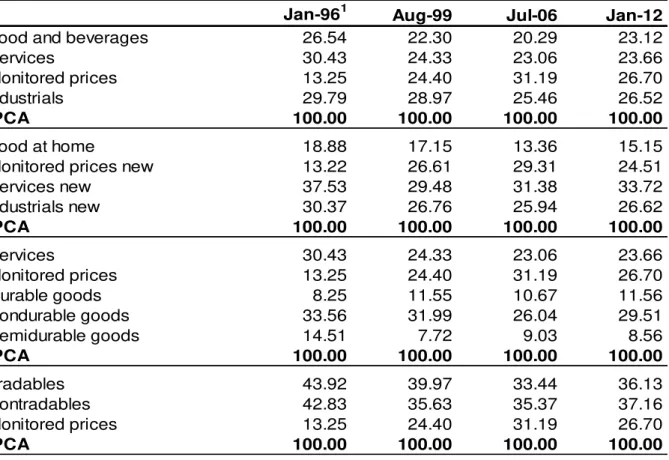
would have given 23.66% for the same period. Table 1 presents the changes of
weighting for each instance of change in the structures of the IPCA because of POF
changes.8 One of the classifications that draws the most attention is that of monitored
prices, given the great weighting change over the period. At the beginning of the review
period, in January 1996, the share of monitored prices was only 13.25%, reaching
31.29% in July 2006, but being greatly reduced in the last weighting change in January
2012 to 26.70%.
7
These changes are significant because the subgroup "Food away from home", despite being a service, may suffer a major influence of the variation in food prices, which are more volatile, changing the dynamics of the series. Moreover, the subsection "Air tickets," has undergone a relatively recent change in methodology for calculating (February 2010), which led to increased volatility of the sub-item, which despite the small weight because of its high variation rates month to month, may have a significant influence on the final outcome of the group.
8The details of the BCB’s lassifi ations and the differen es with the new lassifi ation an e o tained
from the Box "Updates of the Weighting Structures IPCA and INPC and of IPCA Classifications of the Quarterly Inflation Report of December 2011.Available at
[Table 1 about here]
We will thus employ the IPCA forecasts with the following breakdowns, in
which we will use the names defined in Table 2. With models at the aggregate level, for
the purpose of comparison we will use the state-space methodology and
Markov-Switching, as discussed in the previous sections. An advantage of working with
disaggregated prices, in these cases, is the ability to better control for them due to
changes of weighting in the structures.
[Table 2 about here]
5 RESULTS
Evaluation of the models’ performance was conducted using the out
-of-sample results for forecasts for up to twelve months forward. All series and models
were estimated recursively, starting in January 2008 and ending in March 2012. This
means that with every new piece of information added, the models and all their
parameters were re-estimated to always obtain the "best" model, conditional on
information at that time. In this sense, the sample periods for each estimation varies
according to the final sample, i.e. for evaluating the forecasts of the models one step
ahead the sample is 51 months, while for forecast twelve months ahead the sample is
40. We preferred to use the full sample for each forecast horizon, because the more
informative is the series, the better the results found in MCS.
For the disaggregated models, their subcomponents were re-aggregated
the remaining months ahead these were estimated based on the result of the forecasts in
the previous period.
The loss function used to compare models was the mean squared forecast
error (MSFE) which can be defined as the average difference between the estimated
value and the actual, squared. The advantage of this measure is that the larger projection
deviations receive the highest penalty. It should be reiterated that the MSFE was
calculated upon the number index and not in relation to rate of change, so that the
results which will be presented later have relatively larger absolute values than if
compared in percentage terms.
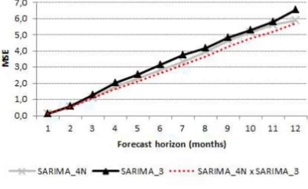
Initial analysis suggests better MSFE performance on more disaggregated
models, while aggregated models showed the worst results. Lower MSFEs were found
in the models with the highest level of disaggregation; the model made by forecasting
the 52 IPCA items (SARIMA_52) is the one with the lowest MSFE, followed by 9
groups subdivisions (SARIMA_9). The third smallest MSFE was the IPCA was
divided into 4 groups: Food and beverages, industrials, services and monitored prices
(SARIMA_4). The largest MSFE's were found in the aggregate models in the three
forecast methods used (SARIMA, Markov-Switching and structural model).
Graphically, the lower performance of the aggregated models compared disaggregated
models becomes even clearer (Figure 1), but the model estimated by state-space
methodology presents the worst results among all models.
We also performed combinations of estimated models, whenever it proved
possible that a combination of forecasts resulted in increased accuracy in terms of the
loss function. To select the possible combinations, we tested using regressions,
following the idea formalized and extended by Chong and Hendry (1986), wherein the
effective value is regressed in function of the forecasts obtained on the basis of the
estimated models plus a constant, and the estimated coefficients cannot be zero nor one,
so that one model overlaps the other. Any value other than that, shows that the joint
forecasts provide useful information about the actual value. The weightings for the
combination were obtained by regression of the estimates of the values achieved
without constant, under the restriction that the sum of the weightings equals one. As
shown by Granger and Ramanathan (1984), this method returns the optimal
variance-covariance outcome. The weights were estimated for all time horizons in order to
always obtain the best combination of templates in each period.
We found five possible combinations that resulted in improved performance
of the combined model compared to the results for each of the individual models.
Among the aggregate models, the combination of the projections of the model estimated
by SARIMA and Markov-switching showed great improvement in performance.
Among the disaggregated models, 4 possible combinations were found, but two of them
showed no improvement on forecasts for all horizons. The combination of the model
disaggregated into 4 groups by the new classification with those disaggregated into 5 or
3 groups showed improvement in all horizons, while the combination of the model
disaggregated in 9 groups showed gains at longer horizons, albeit slight. The
combination of the model disaggregated in 9 groups also showed improvement when
last 5 months. The improvements in the combined results can be better observed in
Figure 2.
[Figure 2 about here]
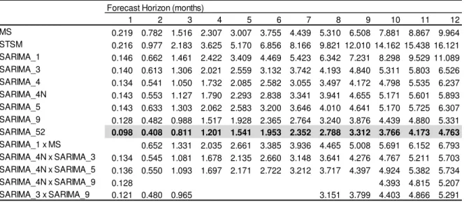
Table 3 below shows the MSFE for all models in forecasts made up to
twelve months ahead. The models are ordered from the lowest level of disaggregation to
greatest possible. At the end of the table are the results obtained by combining the
projections which showed some improvement in terms of the loss function.
[Table 3 about here]
5.1 RESULTS OF MCS
However, only the MSFE analysis alone does not tell us whether the
differences in the models are statistically significant, or if the sample period is
informative enough to define a better model. Thus, we perform statistical tests to see
which models can statistically be considered the best based on the Model Confidence
Set selection criteria. The Table 4 shows all p-values resulting from the MCS and those
models considered part of the set of "best" models ( ), with 90% and 75%
probability, indicated with one and two asterisks respectively, as in Hansen et al (2010).
The results suggest that there is a gain in accuracy in forecasting models
with a higher level of disaggregation, because the IPCA projected in the 52 items
ahead, this model appears as uniquely belonging to . Other evidence that also
suggests a gain from disaggregating is that the model with the second highest degree of
disaggregation, the IPCA projected in all nine groups, appears on in 9 of the 12
forecasts horizons, and for 2, 8, and 12 months forward appears with 90% probability
while for 1, 3, 7, 9, 10, and 11 months ahead appears at 75%. The aggregate models
(MS, STSM and SARIMA_1) fail to appear in MCS, but the combination of the
projections made by the MS and SARIMA_1 models resulted in better performance,
making up part of the MCS in projections between 9 and 12 months ahead. The
combinations of forecasts from models SARIMA_3 and SARIMA_4N showed an
increase in p-value of MCS in relation to models that make up almost all forecast
horizons, except for the first three months. The two combinations performed with the
model SARIMA_9, the second most disaggregated level, showed p-values of MCS
nearly equal to SARIMA_9, except for 1 and 8 months ahead in combination with
SARIMA_3.
[Table 4 about here]
It is quite interesting to note that the gains made in the disaggregated
models occur at all forecast horizons, both the short term and in the longer spans. It
should be noted that the p-values found in the disaggregated models are higher, and the
forecast on the highest level of disaggregation appears with a p-value equal to 1 in all 12
Remember that all estimated models are univariate and multivariate models
that can provide an additional gain. Analysis of multivariate models is one suggestion
for future studies on the topic.
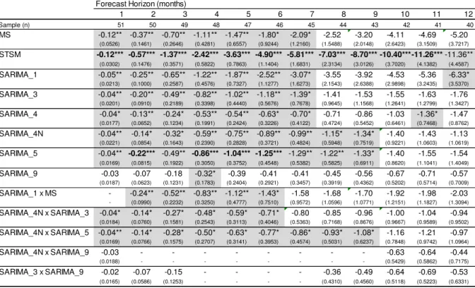
5.2 COMPARING MCS WITH TEST OF DIEBOLD & MARIANO (1995)
The methodology of Diebold-Mariano (DM) for comparing models requires
a benchmark model for the pair-to-pair comparison of forecasting models. We chose to
use as the benchmark the IPCA model composed of 52 items (SARIMA_52), since we
find evidence of gains in accuracy in forecasts using the most disaggregated models.
Thus, we will compare the mean squared forecast errors for SARIMA_52 against all
other models, making sure that the gains are statistically significant for DM. The test
proposed by DM has as null hypothesis of equal forecast performance. The test statistic
is defined by:
(11)
where:
, is the differential loss of function; ;
is a consistent estimator ;
; and .
Thus, the null hypothesis tests at : that is, the differential function
or loss is not significant. The table below presents all tests, using the SARIMA_52
performance gain in the forecast for more disaggregated models. In the shorter-term
forecasts, to 7 months, only the IPCA group (SARIMA_9) models and combinations
thereof are statistically equivalent to at least 10% of significance in relation to the
benchmark, with the exception of the 4-month forecast. All other models are inferior to
the SARIMA_52 model at a 10% significance level. Over longer terms, there is no clear
evidence of improvements from disaggregation, and the only model which declines in
forecast performance at all terms is the structural model.
[Table 5 about here]
6 POSSIBLE EXTENSIONS AND LIMITATIONS OF THE WORK
This study examines forecasts from a broader level of disaggregation of
Brazilian inflation models, and for comparing the forecasting models we used a recent
technique presented by Hansen et al (2010). Nevertheless, there remain some limitations
as well as possibilities for various extensions by future studies. One limitation of the
study lies in the relatively short sample in historical terms, especially when one
considers that the forecasts began in January 2008, losing 51 data points, and also the
series experienced some turbulence due to the change of exchange rate regime in
January 1999 and the relevant currency devaluation in 2002. Another observation
should be made regarding the forecast period, which incorporates several exogenous
shocks such as the financial crisis marked by the bankruptcy of Lehman Brothers in
accommodative monetary policies in developed countries; and the European debt crisis,
with the first request for the IMF bailout of Greece in April 2010. The projection period
also generated a relatively short sample mean square forecast errors, 51 data points for
forecasts one month ahead and 40 for data 12 months ahead, which could compromise
the evaluation due to the real difference in accuracy of the models studied. However,
one of the advantages of MCS is to recognize the limitations of the data, and if these are
not adequately explanatory an MCS with all models would be generated. Thus, a
possible extension of the work would accomplish the same forecasting exercise for
different periods of the IPCA series in order to see whether similar results are obtained
in other periods.
Another possible extension to the work would be to incorporate a wider
range of forecasting models, including multivariate VAR models, Phillips curve
aggregated and disaggregated models, and factorial models, for example. Regarding the
model with the highest level of disaggregation, SARIMA_52, it would be possible to
estimate each item with the model that best fits the series, not just the SARIMA class of
models, which could lead to an even greater gain in disaggregation data.
There is a very large range of possible extensions to the work that could
result in additional gains for research methodologies on Brazilian inflation forecasts.
7 CONCLUSION
This paper presents a comparison of inflation forecasts for up to 12 months
ahead, as measured by the IPCA, using univariate linear and nonlinear time series,
projecting rates from aggregated and disaggregated information. A comparison of the
performance of the forecasts was conducted by Model Confidence Set, introduced by
disaggregated inflation forecasts, more clearly for shorter forecasting horizons, and less
significantly for longer horizons. The analysis by the MSFE and p-value of MCS
suggests that disaggregation offers a performance gain even for longer time horizons,
although these have not been shown to be statistically significant. One factor that may
have limited the results showing significance for longer horizons is the relatively short
sample, both in-sample and for the out-of-sample forecasts. The nonlinear models
estimated for the aggregated IPCA, Markov-switching, and Structural model showed
the worst results among the models. The worst forecast performance was presented by
the Structural model, suggesting that models with stochastic coefficients can generate
results within the sample that are not repeated out-of-sample. The combination of the
forecasts of aggregate models showed significant improvement in the performance of
forecasts, something that was not as evident in the combination of the forecasts of
disaggregated models.
The results presented in the previous section are somewhat similar to those
found in some international work, which showed gains through disaggregation of
forecasts, such as Duarte and Rua (2007), who found an inverse relationship between
amount of information and forecast horizon: i.e. more disaggregated models had better
predictive power in shorter terms. Hubrich and Hendry (2006) also found gains through
disaggregation for forecasting inflation in the Eurozone. Sachsida, Ribeiro and Dos
Santos (2009) found the Markov-switching model poorly suited to forecast Brazilian
quarterly inflation.
The work aims to contribute to the literature emphasizing that the
disaggregated analysis of price indices can generate more accurate forecasts. The results
APPENDIX I - COMPATIBILIZATION OF STRUCTURES OF IPCA ITEMS
Code Item Jan/1991 to Jul/1999 Aug/1999 to Jun/2006 from Jul/2006
3301 Maintenance and repair services n.d. Item 3301 Maintenance and repair
services
Item 3301 Maintenance and repair services
6203 Health insurance n.d. Item 6203 Health insurance Item 6203 Health insurance
7203 Photography and video recording
Agregation of sub-items 7201011 Camera and 7201011 Photography
acessories
Item 7203 Photography and video recording
Item 7203 Photography and video recording
7201 Recreation
Item Recreation less sub-itens 7201011 Camera e 7201011
Photography acessories
Item 7201 Recreation Item 7201 Recreation
8101 Courses
Agregation of sub-items: 7301004. Textbooks; 7301006.Formal courses;
7301020.Books and technical journals; 7301021.Nursery
Item 8101. Courses less sub-item
8101014. Courses in general Item 8101 Cursos
8104 Courses in general Sub-item 7301007.Courses in general Sub-item 8101014.Courses in
general Item 8104 Courses in general
8103 Stationery articles
Agregation of sub-items: 7301002.Notebooks; 7301003.Stationery articles
Item 8103 Stationery articles Item 8103 Stationery articles
9101 Communication Item 5201 Communication Item 9101.Communication Item 9101.Communication
REFERENCES
AKAIKE, H. (1973). Information theory and an extension of the likelihood principle. In B. Petrov and F. Czaki (Eds.), Second International Symposium on Information Theory, pp. 267{287. Budapest: Akademia Kiado.
AREOSA, W. D.; MEDEIROS, M. (2007). Inflation dynamics in Brazil: the case of a small open economy. Brazilian Review of Econometrics, v. 27(1), May, p. 131–166.
ARRUDA, E. F.; FERREIRA, R. T.; CASTELAR, I. (2011). Modelos lineares e não lineares da curva de Phillips para previsão da taxa de inflação no Brasil. Rev. Bras. Econ.
[online]. Vol.65, n.3, pp. 237-252. ISSN 0034-7140. http://dx.doi.org/10.1590/S0034-71402011000300001.
BATES, J.M.; GRANGER, C.W.J. (1969). The combination of forecasts. Operations Research Quarterly 20, 451-468.
BENALAL, N.; DIAZ DEL HOYO, J. L.; LANDAU, B.; ROMA, M.; SKUDELNY, F. (2004). To aggregate or not to aggregate? Euro area inflation forecasting, Working Paper 374, European Central Bank.
BERNANKE, B. (2007). Inflation expectations and inflation forecasting, Speech at the Monetary Economics Workshop of the NBER Summer Institute.
BERNANKE, B.; BOIVIN, J.; ELIASZ, P. (2005). Measuring the effects of monetary policy: a factor-augmented vector autoregressive (FAVAR) approach. Quarterly
Journal of Economics 120, 387–422.
BIDARKOTA, P. V. (2001). Alternative regime switching models for forecasting inflation. J. Forecast., 20: 21–35. doi:
10.1002/1099-131X(200101)20:1<21::AID-FOR763>3.0.CO;2-0
BIDARKOTA, P. V.; MCCULLOCH, J. H. (1998), Optimal univariate inflation forecasting with symmetric stable shocks. J. Appl. Econ., 13: 659–670. doi:
10.1002/(SICI)1099-1255(199811/12)13:6<659::AID-JAE481>3.0.CO;2-Q
BOGDANSKI, J.; TOMBINI, A. A.; WERLANG, S. R. C. (2001). Implementing inflation targeting in Brazil. Money Affairs / Cemla, Centre for Latin American Monetary Studies, v. 14, n. 1, p. 1-23.
BRUNEAU, C.; DE BANDT, O.; FLAGEOLLET, A.; MICHAUX, E. (2007). Forecasting inflation using economic indicators: The case of France. Journal of Forecasting
26: 1–22.
CASTLE, J.L.; HENDRY, D.F. (2007). Forecasting UK inflation: the roles of structural breaks and time disaggregation. Discussion Paper No.309, Department of Economics, University of Oxford.
CASTLE, J.L.; HENDRY, D.F.; CLEMENTS,M. P. (2011). Forecasting by Factors, by Variables, by Both, or Neither? Working paper, Economics Department, University of Oxford.
CHONG, Y.Y.; HENDRY, D.F. (1986). Econometric evaluation of linear macroeconomic models. Review of Economic Studies 53, 671-690.
CLEMEN, R.T., (1989), Combining forecasts: A review and annotated bibliography. International Journal of Forecasting 5, 559-581.
DIEBOLD, F. X.; MARIANO, R. S. (1995). Comparing Predictive Accuracy.
Journal of Business and Economic Statistics, 13, 253–263.
DOORNIK, J. A.; HENDRY, D. F. (2007). Empirical Econometric Modelling: PcGive 12 Volume I. London: Timberlake Consultants Press.
DUARTE, C.; RUA, A. (2007). Forecasting inflation through a bottom-up approach: how bottom is bottom? Economic Modelling, 24, 941-953.
DURBIN, J.; KOOPMAN, S. J. (2004). Time series analysis by state space methods. Oxford: Oxford University.
ENGLE, R. F.; BROWN, S. J. (1986). Model selection for forecasting. Applied
Mathematics and Computation, Volume 20, Issues 3–4, November 1986, Pages 313-327,
ISSN 0096-3003, 10.1016/0096-3003(86)90009-3.
EVANS M., WACHTEL, P. (1993). Inflation regimes and the sources of inflation uncertainty. Journal of Money, Credit and Banking 25: No. 3, 475 – 520.
GOMEZ, V.; MARAVALL, A. (2001). Automatic modeling methods for univariate series. In D. Pena, G. C. Tiao, and R. S. Tsay (Eds.), A Course in Time Series Analysis. New York, NY: J. Wiley and Sons.
GRANGER, C. W. J.; ANDERSEN, A. P. (1978). Introduction to Bilinear Time Series Models. Vandenhoeck and Puprecht.
HANSEN, P. R. (2005). A Test for Superior Predictive Ability. Journal of
Business and Economic Statistics, 23, 365–380.
HARVEY, D. I.; LEYBOURNE, S. J.; NEWBOLD, P. (1997). Testing the Equality of Prediction Mean Squared Errors. International Journal of Forecasting, 13, 281–
291.
HENDRY, D.F.; HUBRICH, K. (2010). Combining disaggregate forecasts or combining disaggregate information to forecast an aggregate. Working Paper Series1155, European Central Bank.
HENDRY, D. F.; HUBRICH, K. (2006). Forecasting Economic Aggregates by Disaggregates. CEPR Discussion Paper No. 5485. Available at SSRN: http://ssrn.com/abstract=900409
HUBRICH, K. (2005). Forecasting euro area inflation: Does aggregating forecasts by HICP component improve forecast accuracy? International Journal of Forecasting 21(1):
119–136.
INOUE, A.; KILIAN, L. (2006). On the selection of forecasting models. Journal
of Econometrics, 130, 273–306.
KIM, C.J. (1993). Unobserved-component time series models with Markov switching heteroskedasticity: Changes in regime and the link between inflation rates and inflation uncertainty. Journal of Business & Economic Statistics 11: No. 3, 341-349.
KOHN, R. (1982). When is an aggregate of a time series efficiently forecast by its past? Journal of Econometrics (18): 337–349.
LÜTKEPOHL, H., (1984). Forecasting contemporaneously aggregated vector ARMA processes. Journal of Business and Economic Statistics 2 (3), 201–214.
MEHRA, R.K. (1974). Identification in control and econometrics: Similarities and differences. Annals of Economic and Social Measurement, Volume 3, number 1 (1974), Sanford V. Berg, editor (p. 21 - 48)
MOSER, G.; RUMLER, F.; SCHARLER, J. (2007). Forecasting Austrian inflation. Economic Modelling. forthcoming.
NIJMAN, T. E.; PALM, F. C. (1990). Predictive accuracy gain from disaggregate sampling in ARIMA models. Journal of Business & Economic Statistics 8: 405–415.
PALM, F. C.; NIJMAN, T. E. (1984). Missing Observations in the Dynamic Regression Model. Econometrica, 52, 1415-1435.
REID, D.J. (1968). Combining three estimates of gross domestic product. Economica, 35, 431-444.
REID, D.J. (1969). A comparative study of time series prediction techniques on economic data. Ph.D. thesis (University of Nottingham, Nottingham).
REIJER, A.; VLAAR, P. (2006). Forecasting inflation: An art as well as a science! De Economist 127(1): 19–40.
ROSE, E. (1977). Forecasting aggregates of independent ARIMA processes.
Journal of Econometrics 5: 323-345.
SACHSIDA, A.; MENDONÇA. M. J. (2009). Reexaminando a Curva de Phillips brasileira com dados de seis regiões metropolitanas. Ipea, Texto para Discussão, 2009.
SACHSIDA, A.; RIBEIRO, M.; DOS SANTOS, C. H. (2009). Curva de Phillips e a experiência brasileira. Ipea, Texto para Discussão 1429, 2009
SCHWARTZMAN, F. F. (2006). Estimativa de Curva de Phillips para o Brasil com preços desagregados. Economia Aplicada, v. 10(1), jan. – mar., p. 137-155.
SORENSON, H. W.; ALSPACH, D. L. (1971). Recursive Bayesian estimation using Gaussian sum. Automatica, 7, 465-79.
STOCK, J. H.; WATSON, M. W. (1998).Diffusion indexes. Working Paper 6702, NBER.
STOCK, J. H.; WATSON, M. W. (2002). Macroeconomic forecasting using diffusion indices. Journal of Business and Economic Statistics 20(2): 147–162.
STOCK, J. H.; WATSON, M.W. (1999). Forecasting inflation. Journal of
Monetary Economics 44: 293–335.
TIAO, G.; GUTTMAN, A. (1980). Forecasting contemporal aggregates of multiple time series. Journal of Econometrics 12: 219-230.
WHITE, H. (2000). A Reality Check for Data Snooping. Econometrica, 68, 1097–
Table 1 – IPCA weights of the BCB classifications in changes tothe POF
Jan-961 Aug-99 Jul-06 Jan-12
Food and beverages 26.54 22.30 20.29 23.12
Services 30.43 24.33 23.06 23.66
Monitored prices 13.25 24.40 31.19 26.70
Industrials 29.79 28.97 25.46 26.52
IPCA 100.00 100.00 100.00 100.00
Food at home 18.88 17.15 13.36 15.15
Monitored prices new 13.22 26.61 29.31 24.51
Services new 37.53 29.48 31.38 33.72
Industrials new 30.37 26.76 25.94 26.62
IPCA 100.00 100.00 100.00 100.00
Services 30.43 24.33 23.06 23.66
Monitored prices 13.25 24.40 31.19 26.70
Durable goods 8.25 11.55 10.67 11.56
Nondurable goods 33.56 31.99 26.04 29.51
Semidurable goods 14.51 7.72 9.03 8.56
IPCA 100.00 100.00 100.00 100.00
Tradables 43.92 39.97 33.44 36.13
Nontradables 42.83 35.63 35.37 37.16
Monitored prices 13.25 24.40 31.19 26.70
IPCA 100.00 100.00 100.00 100.00
Source: IBGE; Banco Central do Brasil
Table 2 – Estimated models and their breakdowns
Name Composition Model
SARIMA_1 Overall Index SARIMA
SARIMA_9 9 groups SARIMA
SARIMA_52 52 items SARIMA
SARIMA_4 Industrials old, Services old, Monitored old and group Food and Beverages SARIMA
SARIMA_3 Tradables, Non-tradables, Monitored old SARIMA
SARIMA_5 Durables, Semidurables, Non-durables, Services old and Monitored old SARIMA
SARIMA_4N Industrials new, Services new, Monitored new and subgroup Food at home SARIMA
MS Overall Index Markov-Switching
STSM Overall Index Structural Model
Table 3 - Mean Square Forecast Error of the models for the forecast horizon
Forecast Horizon (months)
1 2 3 4 5 6 7 8 9 10 11 12
MS 0.219 0.782 1.516 2.307 3.007 3.755 4.439 5.310 6.508 7.881 8.867 9.964 STSM 0.216 0.977 2.183 3.625 5.170 6.856 8.166 9.821 12.010 14.162 15.438 16.121 SARIMA_1 0.146 0.662 1.461 2.422 3.409 4.469 5.423 6.342 7.231 8.298 9.529 11.089 SARIMA_3 0.140 0.613 1.306 2.021 2.559 3.132 3.742 4.193 4.840 5.311 5.803 6.526 SARIMA_4 0.134 0.541 1.050 1.732 2.085 2.582 3.055 3.497 4.172 4.798 5.535 6.237 SARIMA_4N 0.143 0.553 1.127 1.790 2.293 2.838 3.341 3.941 4.655 5.171 5.601 5.893 SARIMA_5 0.143 0.633 1.303 2.062 2.583 3.200 3.646 4.010 4.641 5.170 5.725 6.307 SARIMA_9 0.128 0.482 0.988 1.517 1.928 2.365 2.764 3.240 3.876 4.439 4.880 5.331 SARIMA_52 0.098 0.408 0.811 1.201 1.541 1.953 2.352 2.788 3.312 3.766 4.173 4.763
SARIMA_1 x MS 0.652 1.331 2.035 2.661 3.385 3.936 4.465 5.008 5.691 6.152 6.793 SARIMA_4N x SARIMA_3 0.134 0.545 1.081 1.678 2.135 2.660 3.148 3.641 4.276 4.767 5.211 5.703 SARIMA_4N x SARIMA_5 0.136 0.550 1.093 1.697 2.171 2.722 3.212 3.717 4.397 4.924 5.382 5.734
SARIMA_4N x SARIMA_9 0.128 4.393 4.815 5.207
SARIMA_3 x SARIMA_9 0.121 0.480 0.965 3.151 3.799 4.403 4.866 5.291 Note: The shaded areas and in bold denotes de mininum EQM
Table 4 - Model Confidence Set and p-value of the estimated models
Forecast Horizon (months)
Sample (n) 51 50 49 48 47 46 45 44 43 4 41 40
MS 0,018 0,016 0,011 0,002 0,002 0,009 0,022 0,052 0,059 0,055 0,063 0,049 STSM 0,005 0,009 0,006 0,000 0,000 0,000 0,001 0,002 0,002 0,006 0,005 0,000 SARIMA_1 0,059 0,042 0,019 0,001 0,000 0,003 0,013 0,031 0,025 0,006 0,005 0,007 SARIMA_3 0,106 ** 0,122 ** 0,030 0,015 0,011 0,027 0,051 0,127 ** 0,142 ** 0,164 ** 0,127 ** 0,305 *
SARIMA_4 0,133 ** 0,206 * 0,152 ** 0,049 0,032 0,038 0,070 0,190 ** 0,171 ** 0,193 ** 0,120 ** 0,240 *
SARIMA_4N 0,024 0,242 * 0,152 ** 0,049 0,026 0,023 0,063 0,093 0,106 ** 0,154 ** 0,152 ** 0,431 *
SARIMA_5 0,059 0,035 0,038 0,005 0,004 0,012 0,031 0,103 ** 0,118 ** 0,140 ** 0,120 ** 0,431 *
SARIMA_9 0,140 ** 0,262 * 0,183 ** 0,062 0,066 0,095 0,151 ** 0,286 * 0,187 ** 0,199 ** 0,183 ** 0,521 *
SARIMA_52 1,000 * 1,000 * 1,000 * 1,000 * 1,000 * 1,000 * 1,000 * 1,000 * 1,000 * 1,000 * 1,000 * 1,000 *
SARIMA_1 x MS 0,068 0,067 0,006 0,006 0,014 0,037 0,078 0,106 ** 0,128 ** 0,112 ** 0,254 *
SARIMA_4N x SARIMA_3 0,097 0,198 ** 0,152 ** 0,062 0,041 0,049 0,087 0,198 ** 0,180 ** 0,199 ** 0,183 ** 0,464 *
SARIMA_4N x SARIMA_5 0,080 0,198 ** 0,152 ** 0,062 0,032 0,038 0,070 0,127 ** 0,160 ** 0,193 ** 0,178 ** 0,464 *
SARIMA_4N x SARIMA_9 0,140 ** 0,199 ** 0,183 ** 0,521 *
SARIMA_3 x SARIMA_9 0,148 ** 0,262 * 0,183 ** 0,301 * 0,196 ** 0,199 ** 0,183 ** 0,521 *
7 8 9 10 11 12
1 2 3 4 5 6
Note: The forecasts in is identified by one asterisk and p-value in bold in the shaded area, while those in is identified by two asterisks and p-value in the shaded area.
Forecast Horizon (months)
1 2 3 4 5 6 7 8 9 10 11 12
Sample (n) 51 50 49 48 47 46 45 44 43 42 41 40
MS -0.12** -0.37** -0.70** -1.11** -1.47** -1.80* -2.09* -2.52 -3.20 -4.11 -4.69 -5.20
(0.0526) (0.1461) (0.2646) (0.4281) (0.6557) (0.9244) (1.2160) (1.5488) (2.0148) (2.6423) (3.1509) (3.7217)
STSM -0.12*** -0.57*** -1.37*** -2.42*** -3.63*** -4.90*** -5.81*** -7.03*** -8.70*** -10.40***-11.26***-11.36**
(0.0302) (0.1476) (0.3571) (0.5822) (0.7863) (1.1404) (1.6831) (2.3134) (3.0126) (3.7020) (4.1382) (4.4587)
SARIMA_1 -0.05** -0.25** -0.65** -1.22** -1.87** -2.52** -3.07* -3.55 -3.92 -4.53 -5.36 -6.33*
(0.0213) (0.1000) (0.2587) (0.4576) (0.7327) (1.1277) (1.6273) (2.1543) (2.6388) (2.9898) (3.2435) (3.5370)
SARIMA_3 -0.04** -0.20** -0.49** -0.82** -1.02** -1.18** -1.39* -1.41 -1.53 -1.55 -1.63 -1.76
(0.0201) (0.0910) (0.2189) (0.3398) (0.4440) (0.5676) (0.7678) (0.9645) (1.1568) (1.2641) (1.2799) (1.3427)
SARIMA_4 -0.04* -0.13** -0.24* -0.53** -0.54** -0.63* -0.70* -0.71 -0.86 -1.03 -1.36* -1.47
(0.0177) (0.0652) (0.1234) (0.1991) (0.2424) (0.3226) (0.4122) (0.4724) (0.5452) (0.6461) (0.7468) (0.8762)
SARIMA_4N -0.04** -0.14* -0.32* -0.59** -0.75** -0.89** -0.99** -1.15* -1.34* -1.40 -1.43 -1.13
(0.0221) (0.0854) (0.1643) (0.2390) (0.2828) (0.3721) (0.4824) (0.5948) (0.7519) (0.9221) (1.0603) (1.0619)
SARIMA_5 -0.04** -0.22*** -0.49** -0.86*** -1.04*** -1.25*** -1.29** -1.22** -1.33* -1.40 -1.55 -1.54
(0.0169) (0.0815) (0.1922) (0.3050) (0.3752) (0.4548) (0.5382) (0.5825) (0.6911) (0.8620) (1.1041) (1.4049)
SARIMA_9 -0.03 -0.07 -0.18 -0.32* -0.39 -0.41 -0.41 -0.45 -0.56 -0.67 -0.71 -0.57
(0.0187) (0.0623) (0.1231) (0.1783) (0.2404) (0.2921) (0.3457) (0.3919) (0.4362) (0.5202) (0.5714) (0.7009)
SARIMA_1 x MS - -0.24** -0.52** -0.83** -1.12** -1.43* -1.58 -1.68 -1.70 -1.92 -1.98 -2.03
- (0.0990) (0.2232) (0.3250) (0.4777) (0.7510) (0.9572) (1.0596) (1.0771) (1.2151) (1.1827) (1.3094)
SARIMA_4N x SARIMA_3 -0.04* -0.14* -0.27* -0.48* -0.59* -0.71* -0.80 -0.85 -0.96 -1.00 -1.04 -0.94
(0.0184) (0.0760) (0.1581) (0.2543) (0.3113) (0.4046) (0.5363) (0.7168) (0.8676) (0.9667) (0.9589) (0.9502)
SARIMA_4N x SARIMA_5 -0.04** -0.14* -0.28* -0.50* -0.63* -0.77* -0.86* -0.93* -1.08* -1.16 -1.21 -0.97
(0.0169) (0.0766) (0.1575) (0.2707) (0.3141) (0.3953) (0.4574) (0.5031) (0.6237) (0.7848) (0.9742) (1.0964)
SARIMA_4N x SARIMA_9 -0.03 - - - -0.63 -0.64 -0.44
(0.0188) - - - (0.5429) (0.5862) (0.7175)
SARIMA_3 x SARIMA_9 -0.02 -0.07 -0.15 - - - - -0.36 -0.49 -0.64 -0.69 -0.53
(0.0165) (0.0586) (0.1253) - - - - (0.4310) (0.4560) (0.5118) (0.5223) (0.6331)
Note: The coefficients are the constant from the regression of the difference between the MSE of the most disaggregated model (SARIMA_52) and all other models with a constant. The *** stands for a significance level of 1%, ** stands for a significance level of 5% and * stands for a significance level of 10%.