Artificial Intelligence Techniques for river flow forecasting in the Seyhan River Catchment, Turkey

(1)

HESSD

4, 1369–1406, 2007

River flow forecasting in the

Seyhan River Catchment

M. Firat

Title Page

Abstract Introduction

Conclusions References

Tables Figures

◭ ◮

Back Close

Full Screen / Esc

Printer-friendly Version

Interactive Discussion

Hydrol. Earth Syst. Sci. Discuss., 4, 1369–1406, 2007 www.hydrol-earth-syst-sci-discuss.net/4/1369/2007/ © Author(s) 2007. This work is licensed

under a Creative Commons License.

Hydrology and Earth System Sciences Discussions

Papers published inHydrology and Earth System Sciences Discussionsare under

open-access review for the journalHydrology and Earth System Sciences

Artificial Intelligence Techniques for river

flow forecasting in the Seyhan River

Catchment, Turkey

M. Firat

Pamukkale University Civil Engineering Deprt, Denizli, Turkey

Received: 15 May 2007 – Accepted: 17 May 2007 – Published: 6 June 2007

Correspondence to: M. Firat (mfirat@pamukkale.edu.tr)

(2)

HESSD

4, 1369–1406, 2007

M. Firat

Title Page

Tables Figures

◭ ◮

Back Close

Full Screen / Esc

Abstract

The use of Artificial Intelligence methods is becoming increasingly common in the modeling and forecasting of hydrological and water resource processes. In this study, applicability of Adaptive Neuro Fuzzy Inference System (ANFIS) and Artificial Neural Network (ANN) methods, Generalized Regression Neural Networks (GRNN) and Feed

5

Forward Neural Networks (FFNN), for forecasting of daily river flow is investigated and the Seyhan catchment, located in the south of Turkey, is chosen as a case study.

To-tally, 5114 daily river flow data are obtained from river flow gauges station of ¨Uc¸tepe

(1818) on Seyhan River between the years 1986 and 2000. The data set are divided into three subgroups, training, testing and verification. The training and testing data

10

set include totally 5114 daily river flow data and the number of verification data points is 731. The river flow forecasting models having various input structures are trained and tested to investigate the applicability of ANFIS and ANN methods. The results of ANFIS, GRNN and FFNN models for both training and testing are evaluated and the best fit forecasting model structure and method is determined according to criteria of

15

performance evaluation. The best fit model is also trained and tested by traditional statistical methods and the performances of all models are compared in order to get

more effective evaluation. Moreover ANFIS, GRNN and FFNN models are also verified

by verification data set including 731 daily river flow data at the time period 1998–2000 and the results of models are compared. The results demonstrate that ANFIS model is

20

superior to the GRNN and FFNN forecasting models, and ANFIS can be successfully applied and provide high accuracy and reliability for daily River flow forecasting.

1 Introduction

In last decades, the forecasting and modeling of river flow in hydrological processes is

quite important to deliver the sustainable use and effective planning and management

25

of the water resources. In order to estimate hydrological processes such as

(3)

HESSD

4, 1369–1406, 2007

M. Firat

Title Page

Tables Figures

◭ ◮

Back Close

Full Screen / Esc

tation, runoffand change of water level by using existing methods, some parameters

such as the physical properties of the watershed and river network and observed detail data are necessary. In the literature, there have been many approaches such as, Box and Jenkins (1970) methods of autoregressive (AR), auto-regressive moving average (ARMA), auto-regressive integrated moving average (ARIMA), autoregressive, moving

5

average with exogenous inputs (ARMAX), generally used for modeling of river flow. Some of the earliest examples of the AR type of stream flow forecast models include Thomas and Fiering (1962) and Yevjevich (1963). These approaches have employed conventional methods of the time series forecasting and modeling (Owen et al., 2001; BuHamra et al., 2003; Zhang, 2003; Mohammadi et al., 2006; Arena et al., 2006;

10

Komornik et al., 2006; Toth et al., 2000). Artificial neural networks (ANN) have been

recently accepted as an efficient alternative tool for modeling of complex hydrologic

system to the conventional methods and widely used for prediction. Some specific

applications of ANN to hydrology include modeling rainfall-runo_ff process (Sajikumar

et al., 1999), river flow forecasting (Dibike et al., 2001; Chang et al., 2002; Sudheer

15

and Jain; 2004; Dawson et al., 2002), sediment transport prediction (Fırat and G ¨ung ¨or,

2004), and sediment concentration estimation (Nagy et al., 2002). The ASCE Task Committee reports (2000) did a comprehensive review of the applications of ANN in hydrological forecasting context. Jain and Kumar (2007) proposed a new hybrid time series neural network model that is capable of exploiting the strengths of traditional

20

approaches and ANN. Tingsanchali and Gautam (2000) applied ANN and stochastic hydrologic models to forecast the flood in two river basins in Thailand. GRNN method have also been used for many specific studies (Cigizoglu and Alp, 2006; Kim et al., 2004; Ramadhas et al., 2006; Celikoglu and Cigizoglu, 2007; Celikoglu, 2006). On the other hand, fuzzy logic method was first developed to explain the human thinking

25

and decision system by Zadeh (1965). Several studies have been carried out using fuzzy logic in hydrology and water resources planning (Chang et al., 2001; Liong et

al., 2000; Mahabir et al., 2000; Nayak et al., 2004a; S¸ en and Altunkaynak, 2006).

Re-cently, Adaptive Neuro-fuzzy inference system (ANFIS), which consists of the ANN and

(4)

HESSD

4, 1369–1406, 2007

M. Firat

Title Page

Tables Figures

◭ ◮

Back Close

Full Screen / Esc

fuzzy logic methods, have been used for several application such as, database man-agement, system design and planning/forecasting of the water resources (Chen et al.,

2006; Chang et al., 2006; Nayak et al., 2004b; Fırat and G ¨ung ¨or, 2007; Firat, 2007).

The main purpose of this study is to investigate the applicability and capability of ANFIS and ANN methods for modeling of daily river flow. To verify the application of

5

this approach, the Seyhan catchment located in the south part of Turkey is chosen as the case study area. The River Seyhan is one of the most important water re-sources in Turkey. The River Seyhan flow change depends on various impacts such as climatic and hydro-meteorological variables of the basin, water usage for agricultural and hydroelectric energy. The models for modeling of river flow with having various

10

input structures are developed and applied to the forecasting of the flows of the River Seyhan.

2 Adaptive Neural Fuzzy Inference System (ANFIS)

The fuzzy logic approach is based on the linguistic uncertainly expression rather than numerical uncertainty. Since Zadeh (1965) proposed the fuzzy logic approach to

de-15

scribe complicated systems, it has become popular and has been successfully used in various engineering problems, (Chen et al., 2006; Chang et al., 2001; Liong et al.,

2000; Mahabir et al., 2000; Nayak et al., 2004a; Firat, 2007; Nayak et al., 2004b; S¸ en,

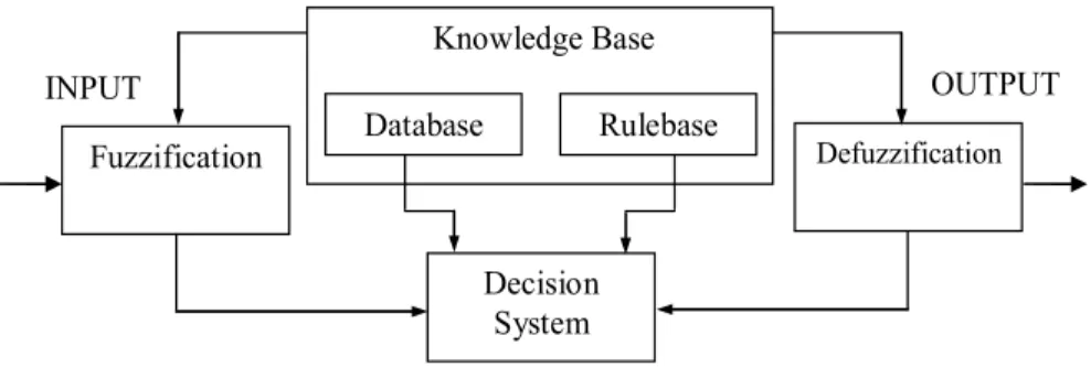
2001). Fuzzy inference system is a rule based system consists of three conceptual components. These are: (1) a rule-base, containing fuzzy if-then rules, (2) a

data-20

base, defining the membership function and (3) an inference system, combining the

fuzzy rules and produces the system results (S¸ en, 2001). The first phase of fuzzy logic

modeling is the determination of membership functions of input – output variables, the second phase is the construction of fuzzy rules and the last phase is the determination

of output characteristics, output membership function and system results (Fırat and

25

G ¨ung ¨or, 2007). A general structure of fuzzy system is demonstrated in Fig. 1.

ANFIS consisting of the combination of the ANN and the fuzzy logic has been shown

(5)

HESSD

4, 1369–1406, 2007

M. Firat

Title Page

Tables Figures

◭ ◮

Back Close

Full Screen / Esc

to be powerful in modeling numerous processes such as rainfall-runoffmodeling and

real-time reservoir operation (Chen et al., 2006; Chang et al., 2006; F_ırat and G ¨ung ¨or,

2007). ANFIS uses the learning ability of ANN to define the input-output relationship and construct the fuzzy rules by determining the input structure. The system results were obtained by thinking and reasoning capability of the fuzzy logic. The

hybrid-5

learning algorithm and subtractive function are used to determine the input structure. The detailed algorithm and mathematical background of these algorithms can be found in Jang et al. (1997). There are two types of fuzzy inference systems, Sugeno-Takagi inference system and Mamdani inference system, in literature. In this study, Sugeno Takagi inference system is used for modeling of daily river flow. The most important

10

di_fference between these systems is the definition of the consequent parameter. The

consequence parameter in Sugeno inference system is a linear equation, called

“first-order Sugeno inference system”, or constant coefficient, “zero-order Sugeno inference

system (Jang et al., 1997). It is assumed that the fuzzy inference system includes two inputs, x and y, and one output, z. For the first-order Sugeno inference system, typical

15

two rules can be expressed as;

Rule 1 : IFx isA₁ and y isB₁ THEN f₁₌p₁∗x₊q₁∗y₊r₁

Rule 2 : IFx isA₂ and y isB₂ THEN f₂₌p₂∗x₊q₂∗y₊r₂

where,x andyare the crisp inputs to the nodei,A_i andB_i are the linguistic labels as

low, medium, high, etc., which are characterized by convenient membership functions

20

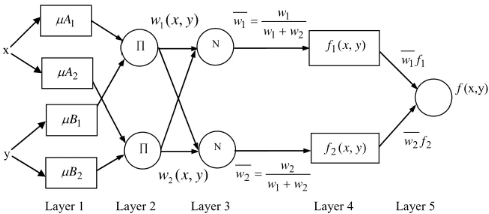
and finally,p_i, q_i andr_i are the consequence parameters. The structure of this fuzzy

inference system is shown in Fig. 2.

Input notes (Layer 1): Each node in this layer generates membership grades of the crisp inputs which belong to each of convenient fuzzy sets by using the membership

functions. Each node’s outputO1_i is calculated by:

25

O1_i₌µ_A

i(x) for i=1,2 ; O 1

i=µBi−2(y) for i=3,4 (1)

(6)

HESSD

4, 1369–1406, 2007

M. Firat

Title Page

Tables Figures

◭ ◮

Back Close

Full Screen / Esc

whereµ_A

i and µBi are the membership functions forAi andBi fuzzy sets, respectively.

Various membership functions can be applied to determine the membership grades. In this study, the Gauss membership function is used, as;

O1_i₌µ_A i(x)=e

−(x−c)2

2σ2 (2)

where, the premise parameters change the shape of membership function from 1 to 0.

5

Rule nodes (Layer 2): In this layer, the AND/OR operator is applied to get one output that represents the results of the antecedent for a fuzzy rule, that is, firing strength.

The outputs of the second layer, called firing strengths O2_i, are the products of the

corresponding degrees obtained from the layer 1, named asw as follows;

O2_i₌w_i₌µ_Ai(x)µ_Bi(y), i₌1,2 (3)

10

Average nodes (Layer 3): Main target is to compute the ratio of firing strength of each

ith rule to the sum firing strength of all rules. The firing strength in this layer is normal-ized as;

O3_i₌w¯_i₌_Pwi

i

w_i i=1,2 (4)

Consequent nodes (Layer 4): The contribution of ith rule towards the total output or

15

the model output and/or the function defined is calculated by Eq. (5);

O4_i₌w¯_if_i₌w¯_i(p_ix₊q_iy ₊r_i) i₌1,2 (5)

where, ¯w_i is theith node output from the previous layer as demonstrated in the third

layer. {p_i, q_i, r_i_}is the parameter set in the consequence function and also the coeffi -cients of linear combination in Sugeno inference system.

20

Output nodes (Layer 5): This layer is called as the output nodes in which the single node computes the overall output by summing all incoming signals and is also the last step of the ANFIS. The output of the system is calculated as;

f(x, y)=w1(x, y)f1(x, y)+w2(x, y)f2(x, y)

w₁(x, y)+w₂(x, y) =

w₁f₁₊w₂f₂

w₁₊w₂ (6)

(7)

HESSD

4, 1369–1406, 2007

M. Firat

Title Page

Tables Figures

◭ ◮

Back Close

Full Screen / Esc

Interactive Discussion Q5_i₌f(x, y)₌X

i

¯

w_i.f_i₌w¯_if₁₊w¯_if₂₌ P

i w_if_i

P

i

w_i (7)

The objective is to train adaptive networks for having convenient unknown functions given by training data and finding the proper value of the input and output parameters. For this aim, ANFIS applies the hybrid-learning algorithm, consists of the combina-tion of the“gradient descent” and “the least-square” methods. The gradient descent

5

method is used to assign the nonlinear input parameters, as the least-squares method is employed to identify the linear output parameters (p_i, q_i, r_i). The “subtractive fuzzy

clustering” function, offering the effective result by less rules, is applied to solve the

problem in ANFIS modeling (Nayak et al., 2004b).

3 Artificial Neural Networks

10

An ANN, can be defined as a system or mathematical model consisting of many non-linear artificial neurons running in parallel which can be generated as one or multiple layered. In this study Generalized Regression Neural Networks (GRNN) and Feed Forward Neural Networks (FFNN) are used for modeling of daily river flow.

3.1 Feed Forward Neural Networks (FFNN)

15

A FFNN consists of at least three layers, input, output and hidden layer. The number of hidden layers and neurons are determined by trial and error method. The schematic diagram of a FFNN is shown in Fig. 3. Each neuron in a layer receives weighted inputs from a previous layer and transmits its output to neurons in the next layer. The summation of weighted input signals are calculated by Eq. (8) and this summation is

20

transferred by a nonlinear activation function given in Eq. (9). The results of network are compared with the actual observation results and the network error is calculated

(8)

HESSD

4, 1369–1406, 2007

M. Firat

Title Page

Tables Figures

◭ ◮

Back Close

Full Screen / Esc

with Eq. (10). The training process continues until this error reaches an acceptable value.

Y_net₌ N X

i=1

Y_i.w_i₊w₀ (8)

Y_out₌f(Y_net)= 1

1+e−Y net (9)

J_r₌1

2.

k X

i=1

(Y_obs−Y_out)2 (10)

5

Y_{out is}the response of neural network system,f(Y_net) is the nonlinear activation function,

Y_netis the summation of weighted inputs,Y_i is the neuron input,w_i is weight coefficient

of each neuron input,w₀ is bias, J_r is the error between observed value and network

result,Y_obsis the observation output value. In this study, the back propagation learning

algorithm, the supervised learning and sigmoid activation function are used in training

10

and testing of models.

3.2 Generalized Regression Neural Networks

A Generalized Regression Neural Networks (GRNN) is a variation of the radial basis neural networks, which is based on kernel regression networks (Cigizoglu and Alp, 2006). A GRNN doesn’t require an iterative training procedure as back propagation

15

networks. A GRNN consists of four layers: input layer, pattern layer, summation layer and output layer as shown in Fig. 4.

The number of input units in input layer depends on the total number of the obser-vation parameters. The first layer is connected to the pattern layer and in this layer each neuron presents a training pattern and its output. The pattern layer is connected

20

to the summation layer. The summation layer has two different types of summation,

(9)

HESSD

4, 1369–1406, 2007

M. Firat

Title Page

Tables Figures

◭ ◮

Back Close

Full Screen / Esc

which are a single division unit and summation units. The summation and output layer together perform a normalization of output set. In training of network, radial basis and linear activation functions are used in hidden and output layers. Each pattern layer unit is connected to the two neurons in the summation layer, S and D summation neurons. S-summation neuron computes the sum of weighted responses of the pattern layer.

5

On the other hand, D summation neuron is used to calculate unweighted outputs of pattern neurons. The output layer merely divides the output of each S-summation neu-ron by that of each D-summation neuneu-ron, yielding the predicted value to an unknown input vector x as (Kim et al., 2004);

Y_i′₌ n P

i=1

y_i.exp [−D(x, x_i)]

n P

i=1

exp [−D(x, x_i)]

(11)

10

D(x, x_i)=

m X

k=1

_x i −xi k

σ 2

(12)

y_i is the weight connection between the ith neuron in the pattern layer and the

S-summation neuron, n is the number of the training patterns, D is the Gaussian function,

m is the number of elements of an input vector, x_k and x_{i k} are the jth element of x

and x_i, respectively, σ is the spread parameter, whose optimal value is determined

15

experimentally.

4 Study area and available data

In this study, the applicability and capability of ANFIS and ANN methods, GRNN and FFNN, is investigated in forecasting and modeling of daily river flow. To illustrate the applicability of the ANFIS and ANN methods, The Seyhan River, located in the south of

20

(10)

HESSD

4, 1369–1406, 2007

M. Firat

Title Page

Tables Figures

◭ ◮

Back Close

Full Screen / Esc

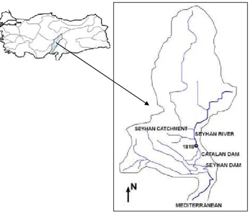
Turkey, is chosen as case study area. It has been operated for irrigation, hydropower generation, domestic use and recreation facilities. The Seyhan River and its drainage basin are shown in Fig. 5.

5 River flow forecasting by Artificial Intelligence Techniques

5.1 Input variables

5

The river flow process in any cross section of river system can be characterized as the function of various variables such as, spatial and temporal distribution of rainfall, catchment and river physical characteristics. The relationship of between river flow and influential variables can be expressed by;

Q(t)₌f(X(t))₊ε_t (13)

10

where, Q(t) denotes the river flow in any cross section of river system, X(t) is the

input vector, which consists of many variables such as spatial and temporal distribution

of rainfall, catchment and river physical characteristics at various time lags, ε_t is the

random error. In the river flow modeling and forecasting, these parameters affects the

performance of the forecasting model because input vector includes the number of

15

antecedent values of these variables. Owing to the complexity of this process, most

conventional approaches are often unable to provide sufficiently accurate and reliable

results. There is one River flow gauging station, Seyhan River ¨Uc¸tepe (1818), equipped

with automatic daily flow recorders, on Seyhan River as shown in Fig. 5. Totally 4383

daily river flow data were obtained from river flow station of ¨Uc¸tepe (1818) on Seyhan

20

River for the time period 1986–2000 and Fig. 6 shows the time series data of daily river flow.

The minimum value; x_min, maximum value; x_max, mean; ¯x, standard deviation; s_x,

variation coefficient c_{v x}, skewness coefficient; c_sx, for total observed data sets are given in Table 1.

25

(11)

HESSD

4, 1369–1406, 2007

M. Firat

Title Page

Tables Figures

◭ ◮

Back Close

Full Screen / Esc

5.2 Model structure

One of the most important steps in developing a satisfactory forecasting model is the selection of the input variables. Hence, cross- correlations between input and output

variables are calculated in order to apply the methods for modeling. Different

combi-nations of the antecedent flows of river flow gauge station are used to construct the

5

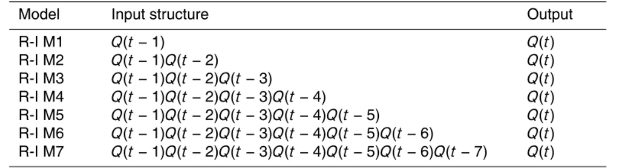
appropriate input structure. The structures of forecasting models are shown in Table 2. Where;Q_t represents the River flow at time (t),Q(t−1),. . .Q(t−n) are the river flow respectively at times (t−1) . . . (t−n). It is evident that the training data sets should

cover all the characters of the problem in order to get effective estimation. The

ob-served data were divided into three parts: training data set, testing data set and

verifi-10

cation data set. The verification data set consisted of the last two years (at time period 1998–2000). The training and testing data set include the daily river flow record at time period 1986–1998 years and the time periods of training/ testing are shown in Table 3. The training and testing experiments with ANFIS and ANN methods are carried out considering various input layer structures with data set given in Fig. 6. The

perfor-15

mances of the models both training and testing data are evaluated and compared

ac-cording to Correlation Coefficient (CORR), Efficiency (E) and Root Mean Square Error

(RMSE).

CORR=

N P

i=1

(Q_D−Q_D).(Q_Y −Q_Y)

s N P

i=1

(Q_D−Q_D)2_.₍_Q

Y −QY)2

(14)

E ₌E1−E2

E₁ E1=

N X

t=1

Q_D−Q_D)2, E₂₌ N X

t=1

(Q_Y−Q_D)2 (15)

20

(12)

HESSD

4, 1369–1406, 2007

M. Firat

Title Page

Tables Figures

◭ ◮

Back Close

Full Screen / Esc

RMSE=

" N X

i₌1

(Q_D−Q_Y)2

N

#0.5

(16)

where,Q_Y is the forecasted river flow,Q_Dis the field observation of river flow,Q_Y is the

average of the forecasted river flows,Q_D is the average of the observation river flow.

The correlation coefficient is a commonly used statistic and provides information on the

strength of linear relationship between the observed and the computed values. The

5

efficiency (E) is one of the widely employed statistics to evaluate model performance.

The values of CORR and E close to 1.0 indicate good model performance. RMSE evaluates the residual between measured and forecasted sediment yield. Theoretically, if this criterion equals zero then model represents the perfect fit, which is not possible at all.

10

5.2.1 ANFIS model

In this study firstly, the seven models having various input variables are trained and tested by ANFIS method and the performances of models for river flow forecasting models are compared and evaluated based on training and testing performances. The best fit model structure is determined according to criteria of performance evaluation.

15

The performances of the ANFIS models are shown in Fig. 7.

As can be seen in Fig. 7, the ANFIS models are evaluated based on their perfor-mance in testing sets. The models have shown significant variations in the criteria of the performance evaluation given in Fig. 5. It shows that the lowest value of the RMSE and the highest values of the RMSE and CORR are R-I M2 ANFIS model. R-I M2

20

ANFIS model, which consists of two antecedent flows in input, has shown the highest

e_fficiency, correlation and the minimum RMSE and R-I M2 was selected as the best-fit

model for modeling of river flow in the Seyhan catchment. The performance of the R-I M2 ANFIS model is shown in Table 4.

It appears that the ANFIS model is accurate and the value of RMSE is small enough,

25

(13)

HESSD

4, 1369–1406, 2007

M. Firat

Title Page

Tables Figures

◭ ◮

Back Close

Full Screen / Esc

and correlation coefficients and efficiencies are very close to unity. The results of the

ANFIS model are compared with the observed flows in order to evaluate the perfor-mance of the training/testing of the model. Figure 8 shows the scatter diagrams of the estimated values of the training/testing of the ANFIS models and observed values.

The results of the ANFIS model demonstrate that the ANFIS can be successfully

5

applied to establish accurate and reliable time series forecasting models. In order to

get a true and effective evaluation of the performance of ANFIS method, the models

were also trained and tested by GRNN and FFNN methods.

5.2.2 ANN models

In this study, secondly, the GRNN and FFNN methods are used for modeling of daily

10

river flow. In the training and testing of ANN models, the same data set is used and performances of models are also evaluated and compared based on given above cri-teria. The performances of the GRNN models are given for both training and testing data sets in Fig. 9.

As can be seen in Fig. 9, the results of all GRNN models trained were compared

15

and evaluated according to their performances in training and testing sets. The values of the E and CORR of R-I M2 GRNN model are higher than those of other models. In addition the value of R-I M2 GRNN model is also lower than that of other models. As a result, R-I M2 GRNN model is selected as the best fit forecasting model according

to criteria of performance evaluation. In order to get a true and effective evaluation,

20

the best fit model structure having two input variables has also been trained and tested by FFNN. The FFNN model having two input variables was trained and tested using the same non-transformed data set. The error backpragation algorithm and sigmoid activation function was used for the training and testing of FFNN model. The number of hidden layers and numbers of hidden neurons in hidden layer, the learning rate, the

25

coefficient of momentum and epochs were selected by trial and error method during

the training. Figure 10 shows the variation of the E, CORR and RMSE criteria with the number of the hidden neurons in hidden layer for testing data sets.

(14)

HESSD

4, 1369–1406, 2007

M. Firat

Title Page

Tables Figures

◭ ◮

Back Close

Full Screen / Esc

As can be seen in Fig. 10, the FNN model, which has five hidden neurons in hidden layer, has shown the best fit performance. The training parameters of the FFNN model

such as, the learning rate (0.02), the coefficient of momentum (0.7) and epochs (2000)

were selected by trial and error method during the training. The performances of R-I M2 GRNN and R-R-I M2 FFNN models are given for both training and testing sets in

5

Table 5, Figs. 11 and 12.

Comparing the performances of GRNN and FFNN forecasting models, it can be seen that the value of the RMSE of the GRNN model is lower than FFNN model. In addition, the values of E and CORR of the GRNN model are also higher than FFNN model. It may be noted that a trial and error procedure has to be performed for FFNN

10

model to develop the best network structure, while such a procedure is not required in developing a GRNN model. The results suggest that the GRNN method is superior to the FFNN method in the modeling and forecasting of the river flow.

5.2.3 Auto-regressive model

In the traditional analysis techniques, the data set must be divided to periodical

com-15

ponent, trend component, internal dependent component and independent (random) components. Trend is the evidence of the increase or decrease of process parame-ters (mean and standard deviation) by time. It is understood that there is a periodical component when the parameters of the process show variation in a determined period. BOX-COX transformation was applied to the data to converge the data to normal

dis-20

tribution. The periodicity of the daily means and standard deviations were calculated by using Fourier series to arrange the periodicity in the data.

DNY(t)= DY(_σt)−DY

DY

(17)

whereDNY(t) is the normalized time series variable, DY(t) is the original time series

variable,DY is the mean of the original time series data and σ_DYis the standard

devi-25

(15)

HESSD

4, 1369–1406, 2007

M. Firat

Title Page

Tables Figures

◭ ◮

Back Close

Full Screen / Esc

R-I M2 model, is used to compare the responses of the R-I M2 ANFIS, ANN models. The structure of AR model can be expressed by following Eq. (18);

Q(t)₌

N X

i=1

α_iQ(t−i)₊ε(t) (18)

where,Q(t) is the daily river flow, Q(t−i) is the river flow at (t−i) time, α is the

auto-regressive parameter to be determined (i) is an index representing the order of AR

5

model andε(t) is the random error. Once the estimates of the traditional time series

model coefficients have been obtained using the training data set, the model can be

validated by computing the performance statistics during both training and testing data sets.

5.2.4 Verification of forecasting models

10

The best fit R-I M2 ANFIS, GRNN and FFNN models are verified by verification data set including totally 731 daily river flow values at the time period 1998–2000 years. The performances of all methods for both testing and verification data sets are given in Table 6.

Comparing verification performances of ANFIS, GRNN and FFNN models, the value

15

of RMSE of ANFIS model is lower than those of GRNN and FFNN model. On the other hand, the values of E and CORR of ANFIS model are also higher than those of GRNN and FFNN models. The results suggest that the ANFIS method is superior to the ANN methods in the modeling and forecasting of river flow. The comp Once the estimates

of the traditional time series model coefficients have been obtained using the training

20

data set, the model can be validated by computing the performance statistics during both training and testing data sets. Comparison of the verification results of models are demonstrated in Fig. 13.

(16)

HESSD

4, 1369–1406, 2007

M. Firat

Title Page

Tables Figures

◭ ◮

Back Close

Full Screen / Esc

6 Conclusions

In this study, applicability and capability of Artificial Intelligence techniques, ANFIS and ANN, for daily river forecasting was investigated. To illustrate the capability of ANFIS and ANN methods, Seyhan River, located in the south of Turkey, was chosen as a case study and estimation models having various input variables were established. The

5

performances of the models and observations were compared and evaluated based on their performance in training and testing sets. The R-I M2 ANFIS model having two antecedent flow variables was selected as the best fit river forecasting model according to criteria of performance evaluation. The models were also trained and tested by GRNN and FFNN methods for the same set of data and results were reported to get

10

more accurate and sensitive comparison. Comparing the results of training and testing of forecasting models, it can be seen that the value of the RMSE of ANFIS model is lower than those of ANN methods, GRNN and FFNN. The values of the E and CORR of ANFIS model are higher than those of GRNN and FFNN models. On the other hand, Comparing verification performances of ANFIS, GRNN and FFNN models, the

15

value of RMSE of ANFIS model is also lower than those of GRNN and FFNN model. In addition, the values of E and CORR of ANFIS model are also higher than those of GRNN and FFNN models. The results suggest that the ANFIS method is superior to the ANN methods in the modeling and forecasting of river flow.

References

20

Arena, C., Cannarozzo, M., and Mazzola, M. R.: Multi-year drought frequency analysis at multiple sites by operational hydrology – A comparison of methods, Phys. Chem. Earth, 31, 1146–1163, 2006.

ASCE Task Committee.: Artificial neural networks in hydrology-II: Hydrologic applications, J. Hydrol. Eng., ASCE 5(2), 124–137, 2000.

25

Box, G. E. P. and Jenkins, G.: Time Series Analysis, Forecasting and Control, Holden-Day, San Francisco, CA, 1970.

(17)

HESSD

4, 1369–1406, 2007

M. Firat

Title Page

Tables Figures

◭ ◮

Back Close

Full Screen / Esc

Interactive Discussion BuHamra, S., Smaoui, N., and Gabr, M.: The Box–Jenkins analysis and neural networks:

prediction and time series modeling, Appl. Math. Model., 27, 805–815, 2003.

Celikoglu, H. B.: Application of radial basis function and generalized regression neural networks in non-linear utility function specification for travel mode choice modeling, Math. Comput. Model., 44, 640–658, 2006.

5

Celikoglu, H. B. and Cigizoglu, H. K.: Public transportation trip flow modeling with generalized regression neural Networks, Adv. Eng. Software, 38, 71–79, 2007.

Chen, S. H., Lin, Y. H., Chang, L. C., and Chang, F. J.: The strategy of building a flood forecast model by neuro-fuzzy network, Hydrol. Processes, 20, 1525–1540, 2006.

Chang, F. J., Hu, H. F., and Chen, Y. C.: Counter propagation fuzzy–neural network for river 10

flow reconstruction, Hydrol. Processes, 15, 219–232, 2001.

Chang, F. J., Chang, L. C., and Huang, H. L.: Real-time recurrent learning neural network for stream-flow forecasting, Hydrol. Processes, 16, 2577–2588, 2002.

Chang, F. J. and Chang, Y. T.: Adaptive neuro-fuzzy inference system for prediction of water level in reservoir, Adv. Water Resour., 29, 1–10, 2006.

15

Cigizoglu, H. K. and Alp, M.: Generalized regression neural network in modelling river sediment yield, Adv. Eng. Software, 37, 63–68, 2006.

Cigizoglu, H. K.: Generalized regression neural network in monthly flow forecasting, Civil Engi-neering and Environmental Systems, 22(2), 71–84, 2005.

Dawson, C. W., Harpham, C., Wilby, R. L., and Chen, Y.: Evaluation of artificial neural network 20

techniques for flow forecasting in the River Yangtze, China, Hydrol. Earth Syst. Sci., 6, 619– 626, 2002,

http://www.hydrol-earth-syst-sci.net/6/619/2002/.

Dibike, Y. B. and Solomatine D. P.: River Flow forecasting Using Artificial Neural Networks, Phys., Chem. Earth (B), 26, 1–7, 2001.

25

Fejer, B. C., Farley, D. T., Woodman, R. F., and Calderon, C.: Dependence of equatorial F-region vertical drift on season and solar cycle, Geophys. Res. Lett., 86, 215–218, 1981. F_ırat, M. and G ¨ung ¨or, M.: Estimation of the Suspended Concentration and Amount by using

Artificial Neural Networks, IMO Technical Journal, 15(3), 3267–3282, 2004.

Fırat, M. and G ¨ung ¨or, M.: River Flow Estimation using Adaptive Neuro-Fuzzy inference System, 30

Mathematics and Computers in Simulation, in press,http://www.sciencedirect.com/science/ journal/03784754, 2007.

Firat, M.: Watershed modeling by adaptive Neuro- fuzzy inference system approach, Ph.D.

(18)

HESSD

4, 1369–1406, 2007

M. Firat

Title Page

Tables Figures

◭ ◮

Back Close

Full Screen / Esc

Interactive Discussion thesis, Pamukkale University, Turkey, (in Turkish), 2007.

Jain, A. and Kumar, A. M.: Hybrid neural network models for hydrologic time series forecasting, Appl. Soft Computing, 7, 585–592, 2007.

Jang, J. S. R, Sun, C. T., and Mizutani, E.: Neuro-Fuzzy and Soft Computing, PrenticeHall, ISBN 0-13-261066-3, 607 s., United States of America, 1997.

5

Kim, B., Lee, D. W., Parka, K. Y., Choi, S. R., and Choi, S.: Prediction of plasma etching using a randomized generalized regression neural network, Vacuum, 76, 37–43, 2004.

Komornik, J., Komornikova, M., Mesiar, R., Sz ¨okeova, D., and Szolgay, J.: Comparison of forecasting performance of nonlinear models of hydrological time series, Phys. Chem. Earth, 31, 1127–1145, 2006.

10

Liong, S. Y., Lim, W. H., Kojiri, T., and Hori, T.: Advance Flood forecasting for Flood stricken Bangladesh with a fuzzy reasoning method, Hydrol. Processes, 14, 431–448, 2000.

Mahabir, C., Hicks, F. E., and Fayek, A. R.: Application of fuzzy logic to the seasonal runoff, Hydrol. Processes, 17, 3749–3762, 2000.

Mohammadi, K., Eslami, H. R., and Kahawita, R.: Parameter estimation of an ARMA model for 15

river flow forecasting using goal programming, J. Hydrol., 331, 293–299, 2006.

Nagy, H. M., Watanabe, K., and Hirano, M.: Prediction of Sediment Load concentration in Rivers using Artificial Neural Network Model, J. Hydrol. Eng., 128, 588–595, 2002.

Nayak, P. C., Sudheer K. P., and Ramasastri, K. S.: Fuzzy computing based rainfall-runoff model for real time flood forecasting, Hydrol. Process, 17, 3749–3762, 2004a.

20

Nayak, P. C., Sudheer, K. P., Ragan, D. M., and Ramasastri, K. S.: A Neuro Fuzzy computing technique for modeling hydrological time series, J. Hydrol., 29, 52–66, 2004b.

Owen, J. S., Eccles, B. J., Choo, B. S., and Woodings, M. A.: The application of auto–regressive time series modelling for the time–frequency analysis of civil engineering structures, Eng. Struct., 23, 521–536, 2001.

25

Ramadhas, A. S., Jayaraja, S., Muraleedharan, C., and Padmakumar, K.: Artificial neural net-works used for the prediction of the cetane number of biodiesel, Renewable Energy, 31, 2524–2533, 2006.

Sajikumar, N. and Thandaveswara, B. S.: A non-linear rainfall–runoffmodel using an artificial neural network, J. Hydrol., 216, 32–55, 2000.

30

Sudheer, K. P. and Jain, A.: Explaining the internal behaviour of artificial neural network river flow models, Hydrol. Processes, 18, 833–844, 2004.

Tingsanchali, T. and Guatam, M. R.: Application of tank, NAM, ARMA and neural network

(19)

HESSD

4, 1369–1406, 2007

M. Firat

Title Page

Tables Figures

◭ ◮

Back Close

Full Screen / Esc

Interactive Discussion models to flood forecasting, Hydrol. Processes, 14, 1362–1376, 1999.

Thomas, H. A. and Fiering, M. B.: Mathematical synthesis of streamflow sequences for the analysis of river basin by simulation, in: Design of Water Resources Systems, edited by: Mass, A., Harvard University Press, Cambridge, MA, 459–493, 1962.

Toth, E., Brath, A., and Montanari, A.: Comparison of short-term rainfall prediction models for 5

real-time flood forecasting, J. Hydrol., 239, 132–147, 2000.

S¸ en Z.: Fuzzy Logic and Foundation, ISBN: 9758509233, 172 p, Bilge K ¨ult ¨ur Sanat Publisher, Istanbul, 2001.

S¸ en Z.: Artificial Neural Network, Water Foundation Publisher, Istanbul, 2004.

S¸ en, Z. and Altunkaynak, A.: A comparative fuzzy logic approach to runoffcoefficient and runoff 10

estimation, Hydrol. Processes, 20, 1993–2009, 2006.

Yevjevich, V.: Fluctuations of Wet and Dry Years, Part-I. Research Data Assembly and Mathe-matical Models, Hydrology Paper 1, Colorado State University, Fort Collins, CO, 1963. Zhang, G. P.: Time series forecasting using a hybrid ARIMA and neural network model,

Neuro-computing, 50, 159–175, 2003. 15

(20)

HESSD

4, 1369–1406, 2007

M. Firat

Title Page

Tables Figures

◭ ◮

Back Close

Full Screen / Esc

Interactive Discussion Table 1.The Statistical Parameters for data sets.

Data Set Variable x_min x_max x¯ s_x c_sx

Training/Testing (1987–1998) Q(t) (m3/s) 54.00 912.00 147.93 110.26 2.26 Verification (1998–2000) Q(t) (m3/s) 60.80 712.00 134.52 95.42 2.37

(21)

HESSD

4, 1369–1406, 2007

M. Firat

Title Page

Tables Figures

◭ ◮

Back Close

Full Screen / Esc

Interactive Discussion Table 2.The structure of the models for forecasting of river flow.

Model Input structure Output

R-I M1 Q(t−1) Q(t)

R-I M2 Q(t−1)Q(t−2) Q(t)

R-I M3 Q(t−1)Q(t−2)Q(t−3) Q(t) R-I M4 Q(t−1)Q(t−2)Q(t−3)Q(t−4) Q(t) R-I M5 Q(t−1)Q(t−2)Q(t−3)Q(t−4)Q(t−5) Q(t) R-I M6 Q(t−1)Q(t−2)Q(t−3)Q(t−4)Q(t−5)Q(t−6) Q(t) R-I M7 Q(t−1)Q(t−2)Q(t−3)Q(t−4)Q(t−5)Q(t−6)Q(t−7) Q(t)

(22)

HESSD

4, 1369–1406, 2007

M. Firat

Title Page

Tables Figures

◭ ◮

Back Close

Full Screen / Esc

Interactive Discussion Table 3.The structure of the training and testing data sets.

Date of training set Date of testing set Date of verification set

1 Oct 1986–30 Sep 1994 1 Oct 1994–30 Sep 1998 1 Oct 1998–30 Sep 2000

(23)

HESSD

4, 1369–1406, 2007

M. Firat

Title Page

Tables Figures

◭ ◮

Back Close

Full Screen / Esc

Interactive Discussion Table 4.Comparison of the performances of the R-I M2 GRNN and FFNN models.

Model Testing Data Set Training Data Set

RMSE E CORR RMSE E CORR

R-I M2 ANFIS 26.95 0.941 0.970 29.43 0.945 0.964

(24)

HESSD

4, 1369–1406, 2007

M. Firat

Title Page

Tables Figures

◭ ◮

Back Close

Full Screen / Esc

Models Testing Data Set Training Data Set

R-I M2 GRNN 32.076 0.917 0.952 42.520 0.848 0.921 R-I M2 FFNN 43.830 0.845 0.924 48.475 0.803 0.900

(25)

HESSD

4, 1369–1406, 2007

M. Firat

Title Page

Tables Figures

◭ ◮

Back Close

Full Screen / Esc

Models Testing Data Set Verification Data Set

R-I M2 ANFIS 26.950 0.941 0.970 33.972 0.873 0.935 R-I M2 GRNN 32.076 0.917 0.952 37.189 0.860 0.928 R-I M2 FFNN 43.830 0.845 0.924 43.595 0.808 0.899 R-I M2 AR(2) 38.420 0.840 0.928 39.344 0.823 0.914

(26)

HESSD

4, 1369–1406, 2007

M. Firat

Title Page

Tables Figures

◭ ◮

Back Close

Full Screen / Esc

EGU OUTPUT

Fuzzification

Decision System

Defuzzification

Database Rulebase Knowledge Base INPUT

Fig. 1: The General Structure of the fuzzy Inference System

∏

+

=

+

=

μ

Fig. 1.The general structure of the fuzzy Inference System.

(27)

HESSD

4, 1369–1406, 2007

M. Firat

Title Page

Tables Figures

◭ ◮

Back Close

Full Screen / Esc

Interactive Discussion y

x ∏

) , (

1 x y

w

∏

N

) , (

2 x y

w

1 1f

w

2 2f

w

Layer 1 Layer 2 Layer 3 Layer 4 Layer 5

2 1

1 1

w w

+ =

2 1

2 2

w w

+ =

1

A μ

2

A μ

1

B μ

2

B μ

) , (

1 x y

f

) , (

2 x y

f

f (x,y)

Fig. 2.The scheme of Adaptive Neuro-Fuzzy Inference System.

(28)

HESSD

4, 1369–1406, 2007

M. Firat

Title Page

Tables Figures

◭ ◮

Back Close

Full Screen / Esc

X

1

X

2

X

N

1 M

Y

Input Layer

Hidden Layer

Output

Layer

w

kj

w

ij

Fig. 3.General structure of a FFNN.

(29)

HESSD

4, 1369–1406, 2007

M. Firat

Title Page

Tables Figures

◭ ◮

Back Close

Full Screen / Esc

Input Layer Pattern Layer

Summation

_Layer

Output

_Layer

X1

X2

X

n

Y

y1

y

n

Fig. 4.The general structure of a GRNN.

(30)

HESSD

4, 1369–1406, 2007

M. Firat

Title Page

Tables Figures

◭ ◮

Back Close

Full Screen / Esc

Fig. 5.The Seyhan River and its drainage area.

(31)

HESSD

4, 1369–1406, 2007

M. Firat

Title Page

Tables Figures

◭ ◮

Back Close

Full Screen / Esc

Interactive Discussion The Time Series Data of Daily River Flows

0 300 600 900 1200

1986 1988 1990 1992 _Year 1994 1996 1998 2000

D

ai

ly

Ri

ve

r F

low

(m

3 /s

) Daily River Flow

Fig. 6.The time series data of daily river flow.

(32)

HESSD

4, 1369–1406, 2007

Seyhan River Catchment M. Firat Title Page Abstract Introduction Conclusions References Tables Figures ◭ ◮ ◭ ◮ Back Close

Full Screen / Esc

Performances of ANFIS Models -T esting Data

0.8 0.85 0.9 0.95 1 R -I M 1 R -I M 2 R -I M 3 R -I M 4 R -I M 5 R -I M 6 R -I M 7 Models CO R R 0.8 0.85 0.9 0.95 1 E CORR E

Performances of ANFIS Models -T esting Data

20 30 40 50 60 R -I M 1 R -I M 2 R -I M 3 R -I M 4 R -I M 5 R -I M 6 R -I M 7 Models RM S E RMSE

Performances of ANFIS Models -T raining Data

0.8 0.85 0.9 0.95 1 R -I M 1 R -I M 2 R -I M 3 R -I M 4 R -I M 5 R -I M 6 R -I M 7 Models CO RR 0.8 0.85 0.9 0.95 1 E CORR E

Performances of ANFIS Models-T raining Data

20 30 40 50 60 R -I M1 R -I M2 R -I M3 R -I M4 R -I M5 R -I M6 R -I M7 Models RM S E RMSE

Fig. 7: The Performances of ANFIS models

Fig. 7.The performances of ANFIS models.

(33)

HESSD

4, 1369–1406, 2007

Full Screen / Esc

T esting Data Set

0 200 400 600 800 1000

1 366 731 1096 1461

Data Set (1994-1998)

D a il y F low ( m 3/s )

R-I M2 ANFIS Observation

T esting Data Set- R-I M2 ANFIS

0 250 500 750 1000

Observation Flow (m3/s)

E st im at ed F lo w (m 3/s ) River Flow

T raining Data Set

0 200 400 600 800 1000

1 726 1451 2176 2901

Data Set (1986-1994)

T raining Data Set- R-I M2 ANFIS

0 250 500 750 1000

Observation Flow (m3_/s)

Fig. 8: The results of training and testing of the R-I M2 ANFIS model

Fig. 8.The results of training and testing of the R-I 2 ANFIS model.

(34)

HESSD

4, 1369–1406, 2007

Full Screen / Esc

Interactive Discussion Performances of GRNN Models -T esting Data Set

20 30 40 50 60 R-I M 1 R-I M 2 R-I M 3 R-I M 4 R-I M 5 R-I M 6 R-I M 7 Models RM S E RMSE

Performances of GRNN Models -T est ing Data Set

0.8 0.85 0.9 0.95 1 R -I M 1 R -I M 2 R -I M 3 R -I M 4 R -I M 5 R -I M 6 R -I M 7 Models CO RR 0.8 0.85 0.9 0.95 1 E CORR E

Performances of GRNN Models -T raining Data

20 30 40 50 60 R -I M 1 R -I M 2 R -I M 3 R -I M 4 R -I M 5 R -I M 6 R -I M 7 Models RM S E RMSE

Performances of GRNN Models -T raining Dat a

0.8 0.85 0.9 0.95 1 R-I M 1 R-I M 2 R-I M 3 R-I M 4 R-I M 5 R-I M 6 R-I M 7 Models CO R R 0.8 0.85 0.9 0.95 1 E CORR E

Fig. 9: The Performances of GRNN models

Fig. 9.The performances of GRNN models.

(35)

HESSD

4, 1369–1406, 2007

M. Firat

Title Page

Tables Figures

◭ ◮

Back Close

Full Screen / Esc

Performances of FFNN Models -T est ing Set

0.6 0.7 0.8 0.9 1

3 4 5 6 7 8 9 10 11 12

T he Numbers of Hidden Neurons

CO

RR

0.6 0.7 0.8 0.9 1

E

CORR E

Performances of FFNN Models -T esting Data

30 40 50 60

3 4 5 6 7 8 9 10 11 12 T he Numbers of Hidden Neurons

RM

S

E

RMSE

Fig. 10: The performances of FFNN model for various hidden neurons

Fig. 10.The performances of FFNN model for various hidden neurons.

(36)

HESSD

4, 1369–1406, 2007

Full Screen / Esc

T esting Data Set

0 200 400 600 800 1000

1 366 731 1096 1461

Data Set (1994-1998)

R-I M2 GRNN Observation

T esting Data Set- R-I M2 GRNN

0 250 500 750 1000

0 250 500 750 1000 Observation Flow (m3/s)

T raining Data Set

0 200 400 600 800 1000

1 366 731 1096 1461 1826 2191 2556

Data Set (1986-1994)

T raining Data Set- R-I M2 GRNN

0 250 500 750 1000

0 250 500 750 1000 Observation Flow (m3/s)

Fig. 11. Results of training and testing of R-I 2 GRNN models.

(37)

HESSD

4, 1369–1406, 2007

Full Screen / Esc

T esting Data Set

0 200 400 600 800 1000

1 366 731 1096 1461

Data Set (1994-1998)

R-I M2 FFNN Observation

T esting Data Set- R-I M2 FFNN

0 250 500 750 1000

T raining Data Set

0 200 400 600 800 1000

1 366 731 1096 1461 1826 2191 2556

Data Set (1986-1994)

T raining Data Set- R-I M2 FFNN

0 250 500 750 1000

Fig. 12: Results of training and testing of R-I M2 FFNN models

Fig. 12.Results of training and testing of R-I 2 FFNN models.

(38)

HESSD

4, 1369–1406, 2007

Full Screen / Esc

Verification Data Set

0 200 400 600 800 1000

1 366 731

Data Set (1998-2000)

Verification Data Set- R-I M2 ANFIS

0 250 500 750 1000

0 200 400 600 800 1000

1 366 731

Data Set (1998-2000)

Verification Data Set- R-I M2 GRNN

0 250 500 750 1000

0 200 400 600 800 1000

1 366 731

Data Set (1998-2000)

Verification Data Set- R-I M2 FFNN

0 250 500 750 1000

Fig. 13: Comparison of the verification results of ANFIS and ANN methods

Fig. 13.Comparison of the verification results of ANFIS and ANN methods.