No 657 ISSN 0104-8910
Os artigos publicados são de inteira responsabilidade de seus autores. As opiniões
neles emitidas não exprimem, necessariamente, o ponto de vista da Fundação
The Role of No-Arbitrage on Forecasting:
Lessons from a Parametric Term Structure
Model
∗
Caio Almeida
Graduate School of Economics Getulio Vargas Foundation Praia de Botafogo 190, 11th Floor,
Botafogo, Rio de Janeiro, Brazil Phone: 5521-2559-5828, Fax: 5521-2553-8821,
Jos´e Vicente
Research Department Central Bank of Brazil Av. Presidente Vargas 730, 7th Floor,
Centro, Rio de Janeiro, Brazil Phone: 5521-21895762, Fax: 5521-21895092,
October 30, 2007
Abstract
Parametric term structure models have been successfully applied to innumerous problems in fixed income markets, including pricing, hedging, managing risk, as well as studying monetary policy impli-cations. On their turn, dynamic term structure models, equipped with stronger economic structure, have been mainly adopted to price derivatives and explain empirical stylized facts. In this paper, we combine flavors of those two classes of models to test if no-arbitrage affects forecasting. We construct cross section (allowing arbitrages) and arbitrage-free versions of a parametric polynomial model to an-alyze how well they predict out-of-sample interest rates. Based on U.S. Treasury yield data, we find that no-arbitrage restrictions sig-nificantly improve forecasts. Arbitrage-free versions achieve overall smaller biases and Root Mean Square Errors for most maturities and forecasting horizons. Furthermore, a decomposition of forecasts into forward-rates and holding return premia indicates that the superior performance of no-arbitrage versions is due to a better identification of bond risk premium.
1
Introduction
Fixed income portfolio managers, central bankers, and market participants are in a continuous search for econometric models to better capture the evo-lution of interest rates. As the term structure of interest rates carries out important information about monetary policy and market risk factors, those models might be seen as useful decision-orienting tools. In fact, in a quest to better understand the behavior of interest rates, a large literature on excess returns predictability and interest rates forecasting has emerged1. In
partic-ular, some models are not consistent inter-temporally while others impose no-arbitrage restrictions, and so far the importance of such restrictions on the forecasting context has not been established yet.
Testing the importance of no-arbitrage on interest rate forecasts should be relevant for at least two reasons. First, since imposing no-arbitrage im-plies stronger economic structure, testing how it will affect model ability to capture risk premium dynamics should be of direct concern to researchers. In principle, although we could expect that a more theoretically-sound model would better capture risk premiums, only careful empirical analysis might manage to answer such question. On the other hand, from a practitioner’s viewpoint, testing how no-arbitrage affects forecasting will objectivelly in-forme managers if it is worth to implement more complex interest rate mod-els or not. Since latent factor modmod-els with no economic restrictions usually represent a simpler alternative to be implemented, if no-arbitrage restrictions don’t aggregate practical gains, they do not necessarily have to be enforced. In this paper, we address the above mentioned points by testing how no-arbitrage restrictions affect the forecasting ability and risk premium structure of a parametric term structure model2. We argue that parametric models
1
Fama (1984), Fama and Bliss (1987), Campbell and Shiller (1991), Dai and Singleton (2002), Duffee (2002), and Cochrane and Piazzesi (2005) analyze the failure of the expec-tation hypothesis and the importance of time-varying risk premia. Kargin and Onatski (2007), Bali et al. (2006), Diebold and Li (2006), and Bowsher and Meeks (2006) study different model specifications in a search for adequate forecasting candidates. Ang and Piazessi (2003), Hordahl et al. (2006), Huse (2007), Favero et al. (2007), and M¨onch (2007) relate interest rates and macroeconomic variables through term structure models.
2
are particularly appropriate to test the effects of no-arbitrage on forecasting, since they keep a fixed factor-loading structure that isindependent of the underlying factors’ dynamics. This invariant loading structure implies that across different versions of the model, bond risk premia relate to a common set of underlying factors, i.e. term structure movements. Based on this fixed set of factors, it should be possible to perform a careful analysis of how each model version and no-arbitrage restrictions affect risk premium.
We parameterize the term structure of interest rates as a linear combi-nation of Legendre polynomials. This framework supports flexible factors’ dynamics, including versions that allow for arbitrage opportunities and oth-ers that are arbitrage-free. Focusing the analysis on three-factor models3,
we compare a cross section (CS) version, which allows for the existence of arbitrages, to two affine arbitrage-free versions, one Gaussian (AFG) and the other with one factor driving stochastic volatility (AFSV).
The CS polynomial version is similar to the exponential model adopted by Diebold and Li (2006) to forecast the U.S. term structure of Treasury bonds, i.e. they are both parametric models that don’t rule out arbitrages. On their turn, the arbitrage-free versions of the Legendre model share many charac-teristics with the class of affine models proposed by Duffie and Kan (1996). No-arbitrage restrictions are imposed through the inclusion of conditionally deterministic factors of small magnitude that guarantee the existence of an equivalent martingale probability measure (Almeida 2005). Each arbitrage-free version is implemented with six latent factors: three stochastic, and three conditionally deterministic. Interestingly, by affecting the dynamics of the three basic stochastic factors (“level”, “slope” and “curvature”), the con-ditionally deterministic factors directly affect bond risk premium structure.
More general arbitrage-free versions of the polynomial model exist and could also be analyzed4. However, priming for objectivity and transparency,
a more concise analysis was favored, with choices of Gaussian (AFG) and Stochastic Volatility (AFSV) affine versions motivated by Dai and Singleton
3
Litterman and Scheinkman (1991) show that most of the variability of the U.S. term structure of Treasury bonds can be captured by three factors: level, slope and curva-ture. Many subsequent more recent works have confirmed their findings. An exception is Cochrane and Piazzesi (2005) who find that a fourth latent factor improves forecasting ability.
4
(2002), Duffee (2002), and Tang and Xia (2007). Duffee (2002) elects the three-factor affine Gaussian model as the best (within affine) to predict U.S. bond excess returns. Dai and Singleton (2002) identify that the same Gaus-sian model correctly reproduces the failures of the expectation hypothesis documented by Fama and Bliss (1987) for U.S. Treasury bonds. In contrast, Tang and Xia (2007) show that a three-factor affine model with one factor driving stochastic volatility generates bond risk premium patterns compat-ible with data from five major fixed income markets (Canada, Japan, UK, US, and Germany). A key ingredient to all these findings is the flexible es-sentially affine parameterization of the market prices of risk (Duffee 2002), which we also adopt in our work.
Based on monthly U.S. zero-coupon Treasury data, we analyze the out-of-sample behavior of the three proposed versions under different forecasting horizons (1-month, 6-month, and 12-month). Forecasting results indicate that dynamic arbitrage-free versions of the model achieve overall lower bias and root mean square errors for most maturities, with stronger results holding for longer forecasting horizons. Diebold and Mariano (1995) tests confirm the statistical significance of obtained results.
In order to analyze the effects of no-arbitrage in the risk premium struc-ture, we decompose yield forecasts into forward rates and risk premium com-ponents. The decomposition allows us to identify that the superior forecast-ing performance of arbitrage-free versions is primarily due to a better identi-fication of bond risk premium dynamics. This result represents an important effort in the direction of understanding how no-arbitrage affects forecasting. It also indicates that further analysis with other classes of parametric models should be seriously considered.
Related works include the papers by Duffee (2002), Ang and Piazzesi (2003), Favero et al. (2007), and Christensen et al. (2007). Duffee (2002) tests the ability of affine models on forecasts of interest rates, concluding that completely affine models fail to reproduce U.S. term structure stylized facts, while essentially affine models do a better job due to a richer risk premium structure. While Duffee (2002) analyzes how different market prices of risk specifications affect forecasting in arbitrage-free models, we study how no-arbitrage affects forecasting, what stands for including models that allow for arbitrages in our analysis.
restrictions affect interest rate forecasting, finding that no-arbitrage mod-els, when supplemented with macro data, are more effective in forecasting. Both papers model factor dynamics with a Gaussian VAR structure, while we include stochastic volatility in our analysis, finding it to be relevant to improve forecasting. In addition, both allow for changes in term structure loadings when comparing no-arbitrage models to models allowing for arbi-trages. Those changes in factors and bond risk premiums make it harder to isolate the pure effects of no-arbitrage on forecasting. In contrast, the parametric term structure polynomial model adopted in our work avoids this issue due to its fixed factor-loading structure.
Christensen et al. (2007) obtain a Gaussian arbitrage-free version of the parametric exponential model proposed by Diebold and Li (2006). They em-pirically test their arbitrage-free version and identify that it offers predictive gains for moderate to long maturities and forecasting horizons. Although in this case they keep a fixed factor loading structure as we do, there are interesting differences between the two papers. First, the two papers analyze distinct parametric families, each offering interesting insights on their own. Second, the technique used to derive arbitrage-free versions is quite distinct. While we base our derivations on Filipovic’s (2001) consistency work, which is not attached to the class of affine models, they make use of Duffie and Kan’s (1996) arguments, which are valid only under affine models. Third, they present a Gaussian arbitrage-free version while we also include the im-portant case where volatility is stochastic. Last, in addition to the forecasting analysis, we propose a careful analysis of the risk premium structure, which should be particularly interesting for portfolio managers and risk managers, as a complementing tool.
Our results should be important to managers and practitioners in general. They suggest it should be worth constructing arbitrage-free versions of other parametric models to test their performances as practical forecasting/hedging tools. The techniques adopted to construct arbitrage-free versions of the polynomial model can be found in Filipovic (2001), and can be readily applied to other parametric families, such as variations of Nelson and Siegel (1987), and Svenson (1994) models5, and splines models with fixed knots, among
5
others.
The paper is organized as follows. Section 2 introduces the polynomial model, presenting its CS and arbitrage-free versions. Section 3 explains the dataset adopted, and presents empirical results, including an interesting dis-cussion relating bond risk premium to model forecasting ability. Section 4 offers concluding remarks and possibly extending topics. The Appendix presents details on the arbitrage-free versions of the polynomial model.
2
The Legendre Polynomial Model
Almeida et al. (1998) proposed modeling the term structure of interest rates
R(.) as a linear combination of Legendre polynomials6:
R(t, τ) = X
n≥1
Yt,nPn−1(
2τ
ℓ −1), (1)
where τ denotes time to maturity, Pn is the Legendre polynomial of degree
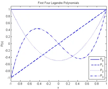
n and ℓ is the longest maturity in the bond market. In this model, each Legendre polynomial represents a term structure movement, providing an intuitive generalization of the principal components analysis proposed by Litterman and Scheinkman (1991). The constant polynomial is related to parallel shifts, the linear polynomial is related to changes in the slope, and the quadratic polynomial is related to changes in the curvature. Naturally, higher-order polynomials are interpreted as loadings of different types of curvatures. For illustration purposes, Figure 1 depicts the first four Legendre polynomials7. This model has been applied to problems involving
scenario-based portfolio allocation, risk management, and hedging with non-paralell movements (see, for instance, Almeida et al. 2000, 2003).
arbitrage-free model.
6
A parametric term structure model based on the power series as opposed to the Leg-endre polynomial basis, appeared before in Chambers et al. (1984). The advantage of Legendre polynomials is that they form an orthogonal basis, being less subject to multi-colinearity problems.
7
They are respectively P0(x) = 1, P1(x) = x, P2(x) = 1 2(3x
2
−1), and P3(x) = 1
2(5x 3
−3x), defined within the interval [-1,1]. The Legendre polynomials of degrees four and five,P4(x) =
1 8(35x
4
−30x2
+3) andP5(x) = 1 8(63x
5
−70x3
On the estimation process, the number of Legendre polynomials is fixed according to some statistical criterion8. When considering zero-coupon yields,
on each date, the model is estimated by running a linear regression of the corresponding vector of observed yields into the set of Legendre polynomials (Pn(·)’s ) previously selected. The cross section version (CS) of the model is
characterized by repeatedly running this linear regression at different instants of time, to extract a time series of term structure movements {Yt}t=1,..,T.
Equipped with those time series one can choose any arbitrary time-series process to fit their joint dynamics. It is important to note, however, that the time-series extraction step imposes no inter-temporal restrictions to term structure movements, consequently allowing for the existence of arbitrages within the model9.
From an economic point of view, it would be interesting to add enough structure to our model so as to enforce absence of arbitrages. To that end, we begin by assuming the following dynamics for the stochastic factors driving term structure movements:
dYt =µ(Yt)dt+σ(Yt)dWt, (2)
where W is a N-dimensional independent standard Brownian motion under the objective probability measureP andµ(·) andσ(·) are progressively mea-surable processes with values inRN and inRN×N, respectively, such that the
differential system above is well-defined.
How do we impose no-arbitrage conditions to the polynomial model? From finance theory, it suffices to guarantee the existence of a martingale measure equivalent to P (see Duffie 2001). More specifically, in order to rule out arbitrage opportunities, and to keep the polynomial term structure form, the following conditions (hereafter denominated AF conditions) must hold
1. The time t price of a bond with time to maturity τ =T −t, B(t, T), should be given by:
B(t, T) = e−τ G(τ)′Yt, (3)
8
Almeida et al. (1998) suggest the use of a stepwise regression, Akaike or Bayesian information criteria.
9
where G(τ) is a vector containing the first N Legendre polynomials evaluated at maturity τ:
G(τ) =
P0
2τ ℓ −1
P1
2τ ℓ −1
. . . PN−1
2τ ℓ −1
′
. (4)
2. There should exist a probability measureQequivalent toP such that, under Q, discounted bond prices are martingales.
The next theorem establishes restrictions (hereafter denominated AF re-strictions10) that will provide arbitrage-free versions of the polynomial model.
Theorem 1 Assume Yt-dynamics under a probability measure Q equivalent
to P given by:
dYt=µQ(Yt)dt+σ(Yt)dWt∗, (5)
where W∗ is a Browian motion under Q.
If µQ(Y
t) satisfies the restriction expressed in Equation 6, Q is an equiv-alent martingale measure and the AF conditions hold11.
(6.1) PN
j=2(j−1)LjYt,jτj−2 =PjN=1LjµQj (Yt)τj−1−P
[N 2] j=1
P[N2]
k=1Γjk(Yt)τ j+k−1
k
(6.2) Γjk(Yt) = 0 for j >[N2] or k >[N2]
(6)
with Γ(Yt) = Lσ(Yt)σ(Yt)L′, Lj standing for the jth-line of an upper tri-angular matrix that depends only on ℓ, and [·] representing the integer part of a number.
Proof and technical details are provided in the Appendix.
The AF restriction has a fundamental implication for any AF version of the Legendre polynomial model: for each stochastic term structure movement there must exist a corresponding conditionally deterministic movement whose
10
The AF restriction is equivalent to imposing the Heath et al. (1992) forward rate drift restriction that ensures absence of arbitrages in the market.
11
In addition to the drift restriction,σ(Yt) should present enough regularity to
guaran-tee that discounted bond prices that are local martingales, also become martingales. In practical problems, a bounded or a square-affineσ(Yt) is enough to enforce the martingale
drift will compensate the diffusion of the former. If we adopt, for instance, a CS version withN factors driving movements of the term structure, the cor-responding arbitrage-free versions should present 2N latent factors in order to become stochastically compatible with CS:N stochastic factors with non-null diffusion coefficients, andN conditionally deterministic factors. Observe that although the AF restriction is enforced to the drift of the risk neutral dynamics (5), in principle, we can work with any general drift (for the firstN
factors) under the objective dynamics (2) by taking general market prices of risk processes. However, the restriction that imposes the existence of condi-tionally deterministic factors must hold under both the risk neutral and the objective measures, and this is what enforces no-arbitrage, and distinguishes AF versions from CS.
In this paper, we focus our analysis on AF versions whose dynamics belong to the class of affine models (Duffie and Kan 1996). This is implemented by restricting the diffusion coefficient of the state vector Y to be within the affine class, simplifying the SDEs for Y to12:
dYt =κQ(θ−Yt)dt+ Σ
p
St(Yt)dWt∗, (7)
where the matrixStis diagonal with elementsStii=αi+βi′Yt for some scalar
αi and some RN-vectorβi.
In the empirical section, we compare a three factor CS version with two AF versions that present three stochastic factors with non-null diffusions. We have seen before that this implies arbitrage-free versions with six factors (three stochastic, three conditionally deterministic). The first AF version is a Gaussian model (βi = 0, ∀i) and the second is a stochastic volatility
model with only one factor driving the volatility. In the Appendix, we show in details how to translate the AF restriction to the affine framework, and further specialize the results to the Gaussian and stochastic volatility AF versions.
Following Duffee (2002) we specify the connection between risk neutral probability measure Q and objective probability measure P through an es-sentially affine market price of risk
Λt=
p
Stλ0+ q
St−λYYt, (8)
12
Note that although bond prices are exponential affine functions of the state space vector Y (see (3)), in general the dynamics of Y is not restricted to be that of an affine model. For instance, if we choose σ(Y) not to be the square root of an affine function of
where λ0 is a N ×1 vector, λY is a N ×N matrix, St appears in Equation
7, and St− is defined by:
Stii−=
1
Sii
t if inf(αi+β t
iYt)>0
0 otherwise.
(9)
The market prices of risk turn out to be of fundamental importance since the dependence of bond expected excess returns ei
t,τ on term structure
move-ments Y is what moves the model away from the Expectation Hypothesis Theory:
eit,τ =−τ G(τ) Σ Stλ0+I−λYYt
. (10)
Equation 10 indicates that zero coupon bond instantaneous expected ex-cess return is a linear combination of model factors, with weights depending on matricesλY, and Σ, and on a predetermined vector of maturity-dependent
Legendre polynomial terms.
Finally, to estimate the parameters of the two AF versions we use a Quasi-Maximum Likelihood procedure since, within the class of affine models, both first and second conditional moments of latent factors are known in closed-form closed-formulas (see Appendix for details).
2.1
Forecasting with the Polynomial Model
Within the sub-class of affine polynomial models with essentially affine mar-ket prices of risk, any arbitrage-free version will correspond to a continuous time vector autoregressive model of order 1 (possibly with stochastic volatil-ity). In order to provide fair comparisons, we match the lagging structure of the time series processes describing arbitrage-free and CS versions, therefore, specializing the CS version to forecast with a VAR(1) process.
The procedure to forecast under the CS version is divided in two steps: First extract the time series YCS
t of term structure movements by running
cross section regressions and then to fit a VAR(1) process to those series of term structure movements:
YCS
t =c+φY CS
t−1+ǫt. (11)
fac-tors under the VAR(1) structure:
Et Y CS t+h
=c
h−1 X
j=0
φj +φhYCS
t . (12)
The conditional expectation of the τ-maturity yield is obtained by substitut-ing factor forecasts in (1):
Et(R(t+h, τ)) = G(τ)′Et Y CS t+h
. (13)
Similarly, for the arbitrage-free affine versions, interest rate forecasts can be produced by using the closed form structure of conditional factor means. As under the affine sub-class the drift of latent factorsYarb.free
can be written as µQ
(Yarb.free t ) = κ
Q
(θ −Yarb.free
t ), the time t conditional expectation of
Yarb.free
t+h is given by (Duffee 2002):
Et Y
arb.free t+h
= (I2N −e−κ Qh
)θ+e−κQhYarb.free
t (14)
where I2N is the identity matrix of order 2N. Finally, for any fixed maturity
τ, the term structure formula in (1) should be used to forecast:
Et(R(t+h, τ)) =G(τ)′Et Y
arb.free t+h
(15)
Under both CS and arbitrage-free versions, forecasts considering horizons longer than the sampling frequency are produced under a multi-step predic-tion structure, as opposed to re-estimating the models under each horizon frequency.
3
Empirical Results
3.1
Data Description
3.2
Estimation
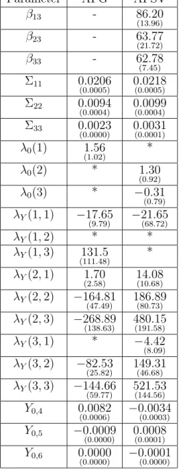
The two AF versions were estimated using a Quasi-Maximum Likelihood procedure, explicitly exploring the fact that the conditional first and sec-ond moments of latent variables are known analytically. Adopting Chen and Scott’s (1993) methodology, a subset of zero-rates (2-, 5- and 10-year ma-turities) was priced without errors, while the remaining rates were priced with i.i.d zero-mean errors. Parameters that identify the stochastic discount factor appear in Table 1. Σ’s and β’s are parameters related to volatility,λ’s are related to factors’ risk premia, and Y0’s define initial conditions for
con-ditionally deterministic factors. Standard deviations from residual fits of 3-and 7-year zeros, indicate that the AFSV version presents a better in-sample cross section fitting than the AFG version (13.6 and 26.0 bps under AFG versus 9.3 and 16.0 bps under AFSV).
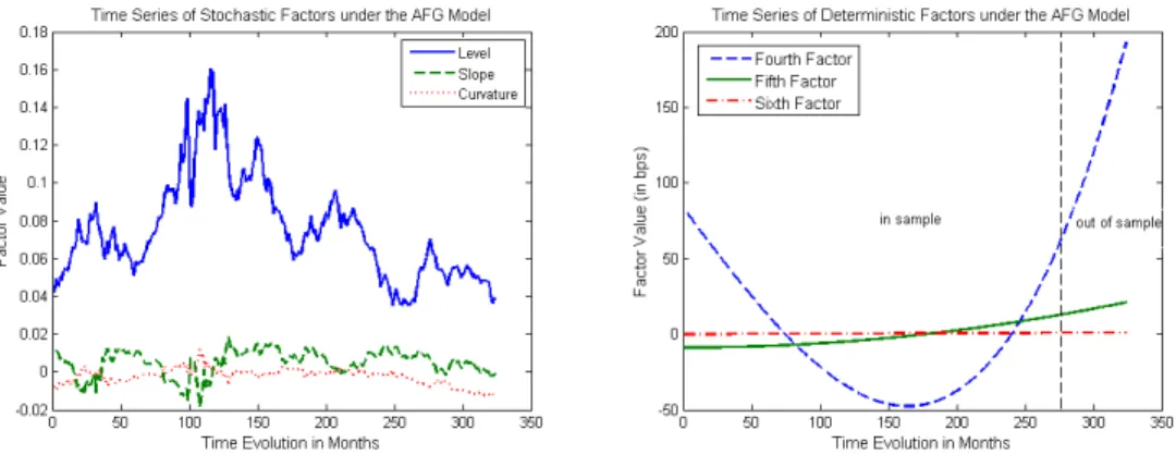
Figures 2 and 3 present time-series of factors capturing term structure movements, for respectively the AFG and AFSV versions. Left-hand side graphs present “level”, “slope” and “curvature” factors. Right-hand side graphs depict the three conditionally deterministic factors. As yields have intrinsic stochastic behavior, it is natural to expect that conditionally de-terministic factors will have their in-sample values minimized by the QML optimization procedure. Indeed, factors five and six, are practically negligible under both arbitrage-free versions. However, factor four, relating to the cubic Legendre polynomial (dashed blue line) gets up to 75 bps under the Gaus-sian version (in-sample), and gets up to 20 bps under the stochastic volatility version (in-sample). It doesn’t vanish like the other two conditionally deter-ministic factors because it represents the “price” that the polynomial model has to pay in order to become arbitrage-free. The three higher order fac-tors change the time-series of lower order movements (“level”, “slope” and “curvature”) in a way to guarantee no-arbitrage under each arbitrage-free version.
The small magnitude of conditionally deterministic factors explains why the three lower order movements present similar time series across different versions of the model (see Figures 2 and 3). Note that the two arbitrage-free versions present the same term structure parametric form, a linear combina-tion of the first six Legendre polynomials, implying that any differences on the time series of the lower order movements should come from differences on the higher order conditionally deterministic factors across versions.
separate cross sectional regressions. While arbitrage-free versions were esti-mated under QML explicitly considering the dynamics of the six polynomial factors, the CS version, in contrast, assumes complete time-independence for factors dynamics, and is based on only the three lower order factors, “level”, “slope” and “curvature”, since conditionally deterministic factors are not necessary in this case, given that no-arbitrage restrictions are not imposed.
Figure 4 presents time-series of the differences between each factor in the CS version (“level”, “slope” and “curvature”), and the corresponding factor on each dynamic version (AFG and AFSV). Those distances are small in mag-nitude and again, come predominantly from the conditionally deterministic factor due to the cubic Legendre polynomial. In fact, for each arbitrage-free version, the shape of the fourth factor time-series is carried out to Figure 413.
3.3
Forecast Comparisons
We proceed as in Section 2.1 to produce, for each version, forecasts based on fixed parameters estimated with the sample ranging from January 1972 to December 199414. We argue that keeping fixed estimated parameters, as
opposed to recursively re-estimating models out-of-sample (like performed in other studies), is an appropriate choice: With fixed estimated parameters, better out-of-sample forecasting suggests higher ability to capture the under-lyind dynamics of interest rates. This choice is consistent with our goal of further analyzing the risk premium structure of the polynomial model.
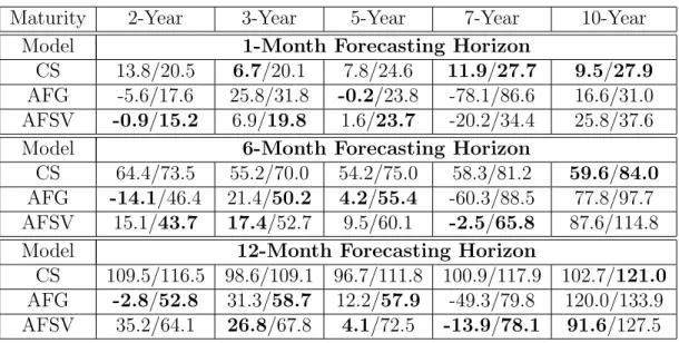
Table 2 presents yield forecast biases and Root Mean Square Errors (RMSE) for the out-of-sample period, from January of 1995 to December of 1998. For each maturity and forecasting horizon h, a total of 49-h forecasts
13
Favero et al. (2007) also compare time-series of term structure movements coming from models with and without no-arbitrage restrictions. They compare movements coming from a Gaussian arbitrage-free model to corresponding movements coming from the Diebold and Li (2006) model, finding that, across models, level factors are more homogenous, while slope and curvature present higher distances.
14
is produced, with h-month ahead forecasts beginning in the hth month of
1995, and ending in December of 1998. Bias and RMSE are measured in ba-sis points, and bold values indicate the lowest absolute value of bias/RMSE under a fixed maturity and forecasting horizon. We first concentrate our analysis on the bias results.
From a total of 15 entries appearing in the table (three forecasting hori-zons and five observed maturities), the CS version presents the lowest abso-lute bias in 4 of them, AFG version in 4, and AFSV in 7. In other words, in more than 70% of the entries the arbitrage-free models present significantly lower biases. Interestingly, the CS version is superior only on the shortest forecasting-horizon (1-month), indicating that no-arbitrage restrictions im-prove longer-horizon forecasts. A more appropriate comparison is proposed by separately comparing CS to each arbitrage-free version. In this case, the AFG version presents absolute bias lower than CS in 9 out of 15 entries, and the AFSV version presents absolute bias lower than CS in 11 out of 15 entries. In summary, from a bias perspective, no-arbitrage tremendously improves results, specially for longer forecasting horizons.
Bias results are pictured in Figure 5, where out-of-sample averaged ob-served and averaged model implied term structures appear. For instance, for a 1-month forecasting horizon, the solid blue line represents an average of the 48 curves that were observed between January 1995 and December of 1998. Correspondingly, the red dotted, the cyan dash-dotted, and the black dashed lines, represent the average of the 48 forecasts produced respectively by CS, AFG, and AFSV versions. The bias is simply the difference between averaged observed and model implied curves. Note how, due to the con-ditionally deterministic factors, arbitrage-free versions present much higher curvature than CS. This higher curvature produces two antagonistic effects: it makes arbitrage-free versions to get much closer to observed yields for most maturities, but also generates strong bias for a few cases15.
Now observing RMSE results in Table 2, it is clear that arbitrage-free versions are again superior. When compared by pairs CS x AFSV and CS x AFG, AFSV is superior to CS in 11 out of 15 entries, and AFG is superior to CS in 9 out of 15 entries. For short-horizon forecasts, the AFSV version presents the best performance, under the RMSE criterion, among the three competitors, and for long-horizon forecasts, AFG takes its place. On its
15
turn, CS version is only better on the 10-year maturity, where arbitrage-free versions are biased due to the conditionally deterministic factors (as mentioned above), and on the short-term forecast of the 7-year yield.
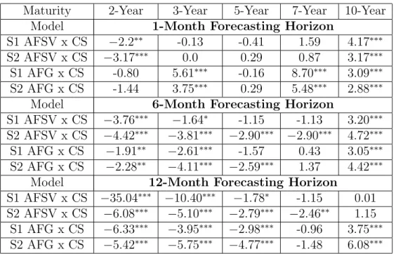
We check the statistical significance of our results by means of the Diebold and Mariano (1995) test. Under a Mean Absolute Error loss function (MAE), Table 3 compares forecasting errors produced with the arbitrage-free versions to corresponding CS forecasting errors16. Negative values of the statistics
(S1 or S2) indicate that no-arbitrage improves forecasts. According to S2,
which is robust to small samples, from a total of 15 table entries, AFSV has forecasting ability superior to CS in 8 of them at a 99% confidence level (bi-caudal test) (in 9 entries at a 95% confidence level). On the other hand, in only 2 entries CS would be superior to AFSV, at both 95% or 99% confidence level. On comparisons between AFG and CS versions, results are more balanced but still in favor of no-arbitrage, with 6 entries in favor of AFG, significant at a 95% confidence level (5 entries at 99%), and 5 entries in favor of CS, at a 99% confidence level. Interestingly, against AFG, CS is strong on short-horizon forecasts and on forecasts for the 10-year yield. Against AFSV, CS is strong only on forecasts for the 10-year yield.
3.4
Discussion
3.4.1 The Effects of Bond Risk Premium in Bias.
In order to better understand the differences in forecasting ability across the three distinct versions of the polynomial model analyzed in this paper, we are interested in decomposing the conditional expectations of yields as the difference of a forward rate component and a bond risk premium component. The bond risk premium component is defined as a holding-return premium, similarly to Hordahl et al. (2006)17.
Suppose we want to analyze model forecasting behavior for a fixed ma-turity of τ years, and forecasting horizon of h months, where one month is our basic time slot. The idea is to consider, at time t, the return of buying a zero-coupon bond with time to maturity τ+ h
12 and selling it hmonths in
the future, leading to the following excess return expression with respect to
16
Significance of results is not affected when we tested with a quadratic loss function.
17
the time t short-term yield with maturity h
12,R(t,
h
12):
BP(τ, h) = Et
"
log B(t+
h
12, τ)
B(t, τ + h
12) ! −R t, h 12 # (16)
We define this holding period return BP to be the bond premium. Now, defining thet1-maturity forward rate, t2 years in the future to be f(t, t1, t2),
the relation between bond premium, corresponding forward rate, and yield conditional expectation is given by:
Et
R
t+ h 12, τ
=f
t, τ, h
12 − h 12 τ !
BP(τ, h) (17)
Equation 17 says that theh-month ahead forecast for the yield with maturity
τ can be directly decomposed as the forward rate of aτ-maturity yield seenh
months in the future, subtracted by a normalized risk premium (normalized by forecasting horizon over time-to-maturity).
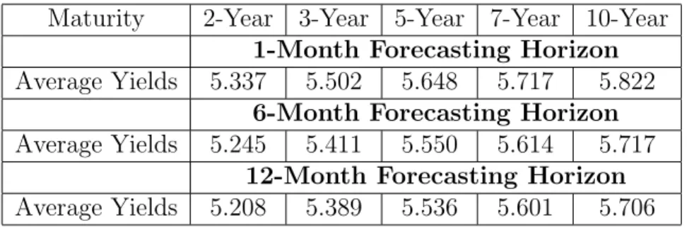
This way, adopting Equation 17, conditional yields are decomposed in a forward rate, and a holding-return premium component. These decomposed forecasts might be useful for managers as an accessing tool to extract risk premium, since there is large interest in obtaining bond premiums from term structure data, and since they are hard to estimate (Kim and Orphanides 2007).
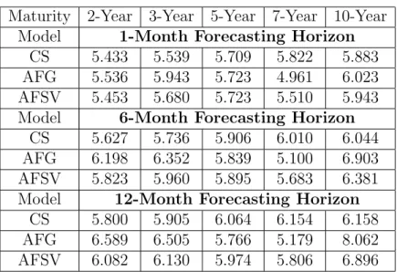
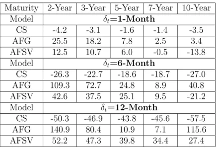
Tables 4, 5, and 6 respectively present out-of-sample averaged yields, av-eraged forward rates, and avav-eraged bond premium. By looking at the first two tables, with a few exceptions, we note that forward rates are higher than average yields, directly indicating that models should present positive risk premium in order to compensate this difference, and to decrease bias. Inter-estingly, Table 6 indicates that both arbitrage-free versions indeed generate positive risk premiums, while in contrast, the CS version generates negative premiums. In other words, under a vector autoregressive structure of lag one, the version that allows arbitrages does not capture risk premium cor-rectly18. For instance, the behavior of the 5-year yield under short/medium term forecasting horizons (1- and 6- month) is of particular interest to our
18
risk premium analysis. The short-term horizon is a good example because forward rates under the three versions of the model are close to each other (see Table 5) implying that differences in bias across versions come pre-dominantly from differences in their implied risk premiums. For a 1-month forecasting horizon, Table 4 shows an averaged observed out-of-sample yield for the 5-year maturity equal to 5.648%19. From Table 5, the 1-month ahead 5-year forward rates are respectively 5.709%, 5.723%, and 5.723%, for CS, AFG, and AFSV versions, with roughly a difference of 1.5 bps between CS and arbitrage-free versions. On the other hand, from Table 6, the averaged risk premiums implied by CS, AFG, and AFSV versions are respectively -1.6, 7.8, and 6.0 bps, indicating that CS misses bond premium even when forward rates are all similar across versions, that is, when we control for dif-ferences in forward rates across versions. Similarly, considering the 6-month forecasting horizon, the 6-month ahead 5 year forward rates for the CS and AFSV versions are very similar, respectively, 5.906% and 5.895% (Table 5), but their implied risk-premiums are very distinct, respectively -18.6 and 25.1 bps (Table 6). It is clear that the forward rates coming from the two versions are overestimating future 5-year yields, but while the positive risk premium implied by the AFSV version corrects this overestimation, the negative risk premium implied by the CS version worsens.
3.4.2 What is the Contribution of No-arbitrage?
Why imposing no-arbitrage leads to better forecasts? The mechanics of the problem can be directly explained by the conditionally deterministic factors. Once they are included in the term structure parameterization, they change the original time series of “level”, “slope” and “curvature” factors, conse-quently affecting the behavior of bond risk premium.
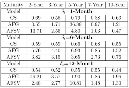
Further appreciation of the no-arbitrage effect on risk premium can be obtained from Table 7. It presents, for each model version, the ratio of the bias generated by assuming a zero bond risk premium (no model implied risk-premium effect), over the true bias generated when model implied bond risk premium is fully incorporated. Whenever risk premium has a positive effect on forecasting, we should immediately observe values higher than 1 for this ratio. For values lower than 1, the model is not correctly capturing
19
the risk premium dynamics. It is particularly interesting to observe that CS presents values lower than 1 in all table entries, indeed confirming that it is not correctly capturing risk premium dynamics. In sparkling contrast, arbitrage-free versions not only present (for most table entries) values higher than 1, but in addition, some entries have values much higher than 120,
indicating that no-arbitrage tremendously increase model ability to correctly capture risk premium dynamics.
A dynamic picture of the risk premium effect described on the paragraph above can be readily observed in Figure 6. For a fixed 12-month forecasting horizon, it presents time-series of observed out-of-sample 2-year yields, with corresponding forward rates, and model implied bond risk premiums21. On
each graph, the dotted line represents observed yields, the dashed line repre-sents the 12-month ahead 2-year forward rate, and the solid line reprerepre-sents the risk premium corrected forward rate, that is, the yield forecast produced with 17. Once risk premium is included, it clearly improves forecasts under the two arbitrage-free versions: the solid line is much closer to the dotted line than the dashed line is. However, under the CS version, risk premium degrades its performance. The dashed line (the one with zero-premium) is much closer to the true observed yield than the solid line (the one including risk premium).
Figure 7 presents examples of risk premium dynamics along the 27 years, from 1972 to 1998, for different maturities and forecasting horizons. The goal of this picture is to show similarities and differences among risk premiums implied by each model version, both in- and out-of-sample. It presents the 1-month holding period return premium for the 5-year bond, the 6-month premium for the 10-year bond, and the 12-month premium for the 2-year bond. Those three maturities give pretty much an idea of the risk premium behavior across the U.S. Treasury term structure for maturities up to 10-years. For the three forecasting horizons, the less volatile premium comes from the AFSV arbitrage-free version. Despite presenting a smaller volatility, it has a very strong effect on improving forecasts as previously observed
20
Under the AFG version, 7 ratio values are higher than 3, and under the AFSV ver-sion, 6 ratio values are higher than 3. A ratio value higher than 3 indicates that once model implied risk premium is considered in forecasting (and not only forward rates), bias decreases for less than one third of the bias value with zero-premium.
21
in Table 7. Risk premiums coming from the other two versions (CS and AFG) have more similar in-sample behavior, but clearly get apart out-of-sample, with the AFG version generating positive premiums, and the CS version generating negative ones. This out-of-sample separation of premiums indicates that while CS might be doing a good job when fitting in-sample data, it is probably overfitting data and missing the true dynamics of yields. The second picture in Figure 7 presents the premium behavior of the 10-year yield under a 6-month forecasting horizon. We have intentionally included this particular maturity to show that even the best arbitrage-free version of the polynomial model (analyzed in this paper) can not capture all features of data, ending up missing the risk premium for this particular maturity. Observe that in the out-of-sample period the AFSV premium converges to approximately the same negative values produced by the CS version, when both should be producing positive premiums. This is a first indication that the polynomial family, at least under its affine subclass, might not be the best candidate to simultaneously describe the behavior of the wholecross section of yields, and to guarantee inter-temporal consistency of the underlying term structure factors.
The third picture in Figure 7 presents the dynamic premium behavior of the 2-year yield under a 12-month forecasting horizon. Note how the out-of-sample behavior of the premium implied under the three versions is tremendously different, with the AFG premium highly positive, AFSV pre-mium slightly positive, and CS prepre-mium highly negative. This distinct dy-namic behavior translates into rather different implications for bias. For instance, the AFG excellent performance when forecasting the 2-year yield 12-months in future (-2.8 bps of bias) can be explained by it risk premium out-of-sample behavior. Picture 2 in Figure 6 indicates that its forward rates are exaggerated with respect to realized yields. However, its out-of-sample risk premium is positive and high, thus compensating those exaggerated for-ward rates, and bringing forecasts to values close to observed yields. On the other hand, AFSV version presents a positive bias of 35.2 basis points, indi-cating that it should have produced higher risk premium values to decrease bias. CS version clearly misses the premium as it should have been positive (see picture 3 in Figure 6), while it is negative during the whole out-of-sample period.
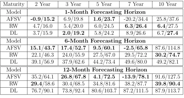
in-tention of putting the polynomial model among credible benchmarks, we present in Table 8, bias and Root Mean Square Errors coming from the best polynomial version AFSV, the established Random Walk (RW) benchmark, and the recently proposed Diebold and Li (2006) model (DL). Forecasting horizons (1-,6-, and 12- month) and maturities (2-, 3-, 5-, 7-, and 10-year) are the same as presented in previous tables. The polynomial model achieves smaller bias and RMSE in 9 out of 15 entries, and, interestingly 7 among those 9 entries are related to longer forecasting horizons (6- and 12-month).
4
Conclusion
We tested the effect of no-arbitrage restrictions on out-of-sample interest rate forecasts. This was implemented with the use of a parametric term structure model that expresses the term structure of interest rates as a linear combination of polynomials. We test this family by comparing forecasts of a model version which admits arbitrages, to two different arbitrage-free versions of the same model, concluding that absence of arbitrage decreases bias and RMSE, specially for longer forecasting horizons.
An important feature of performing this no-arbitrage effect test with a parametric family that presents closed-form formula for bond prices, is that it allows us to isolate the effects of no-arbitrage from other effects like changes in factor loadings under different model dynamic specifications. Fixed factor loadings not only put the forecasting comparison on a fixed basis, but also allow for a similar interpretation of bond risk premia across different model versions. By looking at model implied risk premia, we find that the different versions generate very distinct bond risk premium behavior, whose effect can be directly observed in the out-of-sample forecasting biases. The risk pre-mium implied by arbitrage-free versions improves forward rates forecasting ability while the corresponding premium implied by the cross section version degrades forecasting ability.
factors, out-of-sample22. With this observation in mind, we could conjecture
that under more flexible parametric families, the no-arbitrage restrictions might generate even more positive effects on forecasting. This way, it ap-pears to be room for further evaluation of important parametric families such as the classical polynomial-exponential family whose models by Nelson and Siegel (1987), Diebold and Li (2006), and Svenson (1994) belong to, and also analysis of more complex families like “splines with fixed knots” (see Bowsher and Meeks 2006)23. Moreover, as the techniques used to generate
arbitrage-free versions of parametric models readily allow for inclusion of extra variables in factor dynamics, tests including macroeconomic variables could possibly better identify bond risk premium behavior (see Ludvigson and Ng 2007). We leave those topics for future research.
22
The explosion of these conditionally deterministic factors is exacerbated by the para-metric polynomial structure of the yield curve. A test where all conditionally determin-istic factors are kept at a constant value (their last in-sample value) during the whole out-of-sample period, considerably improves forecasts under both versions, at those “bad” maturities, while keeping the previous good results at other maturities. The results of this test are available upon request.
23
References
[1] Almeida C.I.R (2005). Affine Processes, Arbitrage-Free Term Structures of Legendre Polynomials, and Option Pricing, International Journal of Theoretical and Applied Finance, 8, 2, 1-23.
[2] Almeida C.I.R., A.M. Duarte, and C.A.C. Fernandes (1998). Decompos-ing and SimulatDecompos-ing the Movements of Term Structures of Interest Rates in Emerging Eurobonds Markets. Journal of Fixed Income, 8, 1, 21-31.
[3] Almeida C.I.R., A.M. Duarte, and C.A.C. Fernandes (2000). Credit Spread Arbitrages in Emerging Eurobonds Markets. Journal of Fixed Income,10, 3, 100-111.
[4] Almeida C.I.R , A.M. Duarte, and C.A.C. Fernandes (2003) A Gen-eralization of Principa Component Analysis for Non-observable Term Structures in Emerging Markets, International Journal of Theoretical and Applied Finance, 6, 8, 885-903.
[5] Ang A., and M. Piazzesi (2003). A No-Arbitrage Vector Autoregression of Term Structure Dynamics with Macroeconomic and Latent Variables.
Journal of Monetary Economics, 50, 745-787.
[6] Bali T., M. Heidari, and L. Wu (2006). Predictability of Interest Rates and Interest Rate Portfolios. Working Paper, Baruch College.
[7] Bowsher C. and R. Meeks (2006). High Dimensional Yield Curves: Mod-els and Forecasting. Working Paper, Nuffield College, University of Ox-ford.
[8] Campbell, J. Y. and R. Shiller (1991). Yield Spreads and Interest Rate Movements: A Birds Eye View. Review of Economic Studies, 58, 495-514.
[9] Chambers D.R., W.T. Carleton, and D.W. Waldman (1984). A New Approach to Estimation of the Term Structure of Interest Rates.Journal of Financial and Quantitative Analysis, 19, 3, 233-251.
[11] Chen R.R. and L. Scott (1993). Maximum Likelihood Estimation for a Multifactor Equilibrium Model of the Term Structure of Interest Rates.
Journal of Fixed Income, 3, 14-31.
[12] Christensen J.H.E., F. Diebold, and G.D. Rudebusch (2007). The Affine Arbitrage-free Class of the Nelson-Siegel Term Structure Models. Work-ing Paper, Federal Reserve Bank of San Francisco.
[13] Dai Q. and K. Singleton (2000). Specification Analysis of Affine Term Structure Models. Journal of Finance, LV, 5, 1943-1977.
[14] Dai Q. and Singleton K. (2002). Expectation Puzzles, Time-Varying Risk Premia, and Affine Models of the Term Structure. Journal of Fi-nancial Economics, 63, 415-441.
[15] De Rossi G. (2004). Kalman Filtering of Consistent Forward Rate Curves: A Tool to Estimate and Model Dynamically the Term Struc-ture. Journal of Empirical Finance,11, 277-308.
[16] Diebold F.X. and C. Li (2006). Forecasting the Term Structure of Gov-ernment Bond Yields. Journal of Econometrics, 130, 337-364.
[17] Diebold F.X. and R.S. Mariano (1995). Comparing Predictive Accuracy.
Journal of Business and Economic Statistics, 13, 253-263.
[18] Duffee G. R. (2002). Term Premia and Interest Rates Forecasts in Affine Models. Journal of Finance, 57, 405-443.
[19] Duffie D. (2001). Dynamic Asset Pricing Theory. Princeton University Press.
[20] Duffie D. and Kan R. (1996). A Yield Factor Model of Interest Rates.
Mathematical Finance, 6, 4, 379-406.
[21] Fama E.F. (1984). The Information in the Term Structure of Interest Rates. Journal of Financial Economics, 13, 2, 509-528.
[23] Favero A.C., L. Niu, and L. Sala (2007). Term Structure Forecasting: No-Arbitrage Restrictions vs. Large Information Set. Working Paper, Bocconi University.
[24] Filipovic D. (1999). A Note on the Nelson and Siegel Family. Mathemat-ical Finance, 9, 4, 349-359.
[25] Filipovic D. (2001). Consistency Problems for Heath-Jarrow-Morton Interest Rate Models. Lecture Notes in Mathematics, 1760, Springer-Verlag, Berlin.
[26] Heath D., R. Jarrow and A. Morton (1992). Bond Pricing and the Term Structure of Interest Rates: A New Methodology for Contingent Claims Valuation. Econometrica, 60, 1, 77-105.
[27] Hordahl P., O. Tristani, and D. Vestin (2006). A Joint Econometric Model of Macroeconomic and Term Structure Dynamics. Journal of Econometrics,131, 405-440.
[28] Huse C. (2007). Term Structure Modelling with Observable State Vari-ables. Working Paper, London School of Economics.
[29] Kargin V. and A. Onatski (2007). Curve Forecasting by Functional Au-toregression. Working Paper, Columbia University.
[30] Kim D. and A. Orphanides (2007). The Bond Market Term Premium: What is it, and How can we Measure it?, BIS Quarterly Review, June.
[31] Litterman R. and Scheinkman J.A. (1991). Common Factors Affecting Bond Returns. Journal of Fixed Income, 1, 54-61.
[32] Ludvigson S. and S. Ng (2007). Macro Factors in Bond Risk Premia. Working Paper, Department of Economics, New York University.
[33] McCulloch J.H. (1971). Measuring the Term Structure of interest Rates.
Journal of Business, 44, 19-31.
[35] Nelson C. and A. Siegel (1987). Parsimonious Modeling of Yield Curves.
Journal of Business, 60, 4, 473-489.
[36] Sharef E. and D. Filipovic (2004). Conditions for Consistent Exponential-Polynomial Forward Rate Processes with Multiple Nontriv-ial Factors. International Journal of Theoretical and Applied Finance, 7, 685-700.
[37] Svensson L. (1994). Monetary Policy with Flexible Exchange Rates and Forward Interest Rates as Indicators. Institute for International Eco-nomic Studies, Stockholm University.
[38] Tang H. and Y. Xia (2007). An International Examination of Affine Term Structure Models and the Expectations Hypothesis. Journal of Financial and Quantitative Analysis,42, 1, 41-80.
5
Appendix
5.1
Proof of Theorem 1.
Theorem 1.
Assume Yt-dynamics under a probability measure Q equivalent to P given
by:
dYt=µQ(Yt)dt+σ(Yt)dWt∗, (18)
where W∗ is a Browian motion under Q. If µQ
(Yt) satisfies the restriction expressed in Equation (19), Q is an
equivalent martingale measure and the AF conditions hold24.
PN
j=2(j−1)LjYt,jτj−2 =PjN=1LjµQj (Yt)τj−1−P
[N 2] j=1
P[N2]
k=1Γjk(Yt)τ j+k−1
k
Γjk(Yt) = 0 for j >[N2] or k >[N2]
(19) with Γ(Yt) = Lσ(Yt)σ(Yt)L′, Lj standing for the jth-line of an upper
triangular matrix that depends only on ℓ, and [·] representing the integer part of a number.
Proof of Theorem 1.
The term structure of the Legendre polynomial model is given by:
R(τ, Yt) =G(τ)′Yt= N
X
n=1
Yt,nPn−1(
2τ
ℓ −1), (20)
that is, the loadings of the term structure are Legendre polynomials. There-fore, the τ-maturity instantaneous forward rate is
f(τ, Yt) = N
X
n=1
Yt,nPn−1(
2τ
ℓ −1) +τ
N
X
n=1
Yt,n
∂Pn−1(2ℓτ −1)
∂τ
!
. (21)
In the equation above, the forward rates are expressed as linear combinations of Legendre polynomials, which can be readily expressed as linear
combina-24
In addition to the drift restriction,σ(Yt) should present enough regularity to
guaran-tee that discounted bond prices that are local martingales, also become martingales. In practical problems, a bounded or a square-affineσ(Yt) is enough to enforce the martingale
tions of powers of τ:
f(τ, Yt) = N
X
n=1
LnYtτn−1, (22)
whereLnis thenthrow of the upper triangular matrixL. In fact, (22) defines
matrix L. If N = 6 the matrix L is25
L=
1 −1 1 −1 1 −1
0 4ℓ −12ℓ 24ℓ −40ℓ 60ℓ
0 0 18ℓ2 −
90
ℓ2 270
ℓ2 − 630
ℓ2
0 0 0 80
ℓ3 −560ℓ3 2450ℓ3
0 0 0 0 350ℓ4 −
3150
ℓ4
0 0 0 0 0 1512ℓ5
. (24)
Proposition 3.2 of Filipovic (1999) presents conditions on f(τ, Yt), which
guarantee that discounted bond prices are martingales under any specific in-terest rate model26. Using these conditions, Almeida (2005) proves that if the
AF restrictions (19) hold, then the Legendre polynomial model is arbitrage-free. ⋄
25
Using the first six Legendre polynomials we have
f(τ, Yt) =
Yt,1+Yt,2x+
Yt,3
2 (3x 2
−1) + Yt,4
2 (5x 3
−3x)+
Yt,5
8 (35x 4
−30x2
+ 3) + Yt,6
8 (63x 5
−70x3
+ 15x)+
2τ ℓ
h
Yt,2+ 3Yt,3x+
Yt,4
2 (15x 2
−3)i+
2τ ℓ
hY
t,5
8 (140x 3
−60x) +Yt,6
8 (315x 4
−210x2
+ 15)i.
(23)
wherex= 2τ
ℓ −1. Collecting terms that are powers ofτ in the expression above we obtain
the upper triangular matrixLforN = 6.
26
5.2
Technical Details about the Sub-Class of
Arbitrage-Free Legendre Models with Affine Dynamics.
The affine class of dynamic term structure models is composed by processes whose state vector Y is an affine diffusion27, and whose implied short term
rate is affine in Y. Dai and Singleton (2000) proposed the following notation to describe the dynamics of canonical affine models under the risk neutral measure Q:
dYt =µQ(Yt)dt+ Σ
p
St(Yt)dWt∗ =κ
Q
(θQ−Yt)dt+ Σ
p
St(Yt)dWt∗ (25)
where κQ and Σ areN ×N matrices, θQ is a
RN-vector, and S
t is diagonal
matrix with elements Stii =αi+βi′Yt for some scalar αi and someRN-vector
βi.
Now suppose we want to equip the affine class of models with a loadings structure composed by Legendre polynomials28. To this end, we have to
impose the AF restrictions of Theorem 1.
Consider the auxiliary state space vector ˜Yt defined by
˜
Yt=LYt, (26)
where L is the upper triangular matrix of Theorem 1. This auxiliary pro-cess characterizes term structure movements when the loadings come from a power series in the maturity variable τ. It appears as an intermediate step in calculations.
The dynamics of ˜Yt under probability measure Qis given by
dY˜t= ˜µQ( ˜Yt)dt+ ˜Σ
q
˜
St( ˜Yt)dWt∗, (27)
where the parameters of this stochastic differential equations system are de-fined in similar way to (25) (i.e., ˜Sii
t = ˜αi+ ˜βi
′ ˜
Ytfor some scalar ˜αi and some
RN-vector ˜β
i and so on) and are related through (26) with the corresponding
parameters in (25). It should be clear that ˜Yt is affine if, and only if, Yt is
affine, because L is invertible.
27
This means that the drift and the squared diffusion terms ofY are affine functions of
Y.
28
Under this particular sub-class (affine plus polynomial loadings), the first requirement of AF restrictions becomes
N
X
j=2
(j −1) ˜Yt,jτj−2 = N
X
j=1
µQj ( ˜Yt)τj−1−
[N 2] X
j=1 [N
2] X
k=1
( ˜H0,jk+ ˜H1,jkY˜t)
τj+k−1 k , (28)
where Σ ˜˜StΣ˜′
ij = ˜H0ij+ ˜H1ij
˜
Yt, with ˜H0ij ∈R and ˜H1ij ∈RN.
In particular, by matching coefficients on the maturity variableτ in (28), we obtain an explicit expression for the drift of the auxiliary process:
˜
µQY˜t
i =i
˜
Yt,i+1+
Min{i−1,[N2]}
X
j=Max{1,i−[N2]} ˜
H0,j(i−j)+ ˜H1,j(i−j)Y˜t
i−j . (29)
This expression can be readily translated to a similar expression for the drift of the original state vector Y with the use of (26).
In the empirical section of our paper, we compare a three factor CS ver-sion with corresponding AF verver-sions that present three stochastic factors with non-null diffusions. By Theorem 1, a natural way to implement this ap-plication, is to work with AF versions driven by six factors (three stochastic, three conditionally deterministic). In the next lines, we provide the restric-tions that should be implemented to generate affine models with polynomial
When N = 6 the dynamics of ˜Yt has the following form:
˜
Stii( ˜Yt) =
˜
αi+ ˜β ′
iY˜t if i≤3
0 if i >3,
˜
Σi,j = 0 i, j >3,
˜
µQ
( ˜Yt)1 = ˜Yt,2,
˜
µQ( ˜Yt)2 = 2 ˜Yt,3+ ˜H0,11+ ˜H1,11Y˜t,
˜
µQ( ˜Yt)3 = 3 ˜Yt,4+
˜
H0,12
2 +
˜
H1,12
2 Y˜t+ ˜H0,21+ ˜H1,21Y˜t,
˜
µQ( ˜Yt)4 = 4 ˜Yt,5+
˜
H0,13
3 +
˜
H1,13
3 Y˜t+ ˜
H0,22
2 +
˜
H1,22
2 Y˜t+ ˜H0,31+ ˜H1,31Y˜t,
˜
µQ( ˜Yt)5 = 5 ˜Yt,6+
˜
H0,23
3 +
˜
H1,23
3 Y˜t+ ˜
H0,32
2 +
˜
H1,32
2 Y˜t,
˜
µQ( ˜Yt)6 =
˜
H0,33
3 +
˜
H1,33
3 Y˜t.
(30) The dynamics of the term structure movements Y under the original Legendre polynomial parameterization can then be obtained by solving (26). To that end, let us rewrite the drift ˜µQ
in matrix notation, as an affine transformation of ˜Y:
˜
where U =U1+U2, and U1, U2 and M are given by: M = 0 ˜
H0,11
˜
H0,12
2 + ˜H0,21 ˜
H0,13 3 +
˜
H0,22
2 + ˜H0,31 ˜
H0,23 3 +
˜
H0,32 2
˜
H0,33 3 , (32)
U1 =
0 1 0 0 0 0 0 0 2 0 0 0 0 0 0 3 0 0 0 0 0 0 4 0 0 0 0 0 0 5 0 0 0 0 0 0
, (33)
U2=
01×6
˜
H1,11
˜
H1,12
2 + ˜H1,21 ˜
H1,13 3 +
˜
H1,22
2 + ˜H1,31 ˜
H1,23 3 +
˜
H1,32 2
˜
H1,33 3 . (34)
Finally, the drift and diffusion of process Y are given by:
µQ(Yt) = L−1µ˜Q( ˜Yt) =L−1µ˜Q(LYt) = L−1M +L−1U LYt (35)
and
σ(Yt) = L−1Σ˜
q
˜
In our empirical application, the maximum maturity is equal to ℓ = 10 years. Then, matrix L is given by:
L=
1 −1 1 −1 1 −1
0 0.4 −1.2 2.4 −4 6
0 0 0.180 −0.9 2.70 −6.3
0 0 0 0.08 −0.56 2.24
0 0 0 0 0.035 −0.3158
0 0 0 0 0 0.0152
. (37)
Now we are ready to specialize the drift restriction (30) to each particular AF version implemented in this paper (AFG and AFSV), and also to obtain the corresponding restrictions for the process of interest Y, the one that drives term structure movements within the Legendre polynomial model.
5.2.1 The AFG Version
Noting that in this version the matrix controlling the diffusion structure of vector ˜Y, i.e. ˜S(.), is the identity matrix, we directly obtain ˜Σ ˜Σ′ = ˜H
0, and
from (36) we obtain the relation between ˜H0 and Σ:
˜
H0 =LΣ2((L−1)′)−1 =LΣ2L′. (38)
If we adopt a diagonal matrix representation for Σ29, with Σ
ii as the ith
-diagonal term, then, in order to match the second requirement of AF re-strictions we must have Σii = 0 for i ≥ 4. Therefore, using transformation
L between Y and ˜Y, ˜H0 can be explicitly related to the non-null diagonal
terms in Σ:
29
˜
H0 =
Σ211+ Σ222+ Σ233 −0.4Σ222 −1.2Σ233 −0.18Σ233 0 0 0
−0.4Σ222−1.2Σ233 0.16Σ222+ 1.44Σ233 −0.216Σ233 0 0 0
0.18Σ2
33 −0.216Σ233 0.0324Σ233 0 0 0
0 0 0 0 0 0
0 0 0 0 0 0
0 0 0 0 0 0
. (39)
Since U2 is null under the Gaussian version, we learn from (35) that the
two matrices (L−1M and L−1U
1L) necessary to obtain an explicit expression
for the drift µQ
(Yt) are given by:
L−1M =
5 2Σ 2 11+ 5 6Σ 2 22+ 1 2Σ 2 33 5 2Σ 2 11+ 3 2Σ 2 22+ 11 14Σ 2 33 5 3Σ 2 22+ 5 7Σ 2 33 Σ2
22+ Σ233
9 7Σ 2 33 5 7Σ 2 33 (40) and
L−1U1L=
0 0.4 −0.3 0.56667 −0.41667 0.65667
0 0 0.9 −0.5 1.25 −0.77
0 0 0 1.3333 −0.58333 1.7833
0 0 0 0 1.75 −0.63
0 0 0 0 0 2.16
0 0 0 0 0 0
Note that Y4, Y5, and Y6 are deterministic factors under the Gaussian case.
This is a consequence of two facts: (i) their dynamics do not depend on the Brownian motion vector, and (ii) their drifts do not depend on the first three components of the state vector. With matrices L−1M and L−1U
1L in
hands, we obtain the drift of vector Y, and in particular, the drifts of the deterministic factors Y4, Y5, and Y6:
µQ(Y
t)4 = Σ222+ Σ233+ 1.75Yt,5−0.63Yt,6,
µQ(Yt)5 =
9 7Σ
2
33+ 2.16Yt,6,
µQ(Yt)6 =
5 7Σ
2 33.
(42)
By explicitly solving the ordinary differential equations implied for these factors, we have
Yt,4 =Y0,4+(Σ222+Σ332 +1.75Y0,5−0.63Y0,6)t+(0.9Σ233+0.189Y0,6)t2+0.45Σ233t3,
(43)
Yt,5 =Y0,5+ (
9 7Σ
2
33+ 2.16Y0,6)t+
27 35Σ
2
33t2, (44)
Yt,6 =Y0,6+
5 7Σ
2
33t. (45)
Note that, under this Gaussian version, the dynamics of the state vari-ables Yt,4, Yt,5 and Yt,6, in addition to being deterministic, are completely
determined by parameters Σ22, Σ33, and the initial conditions Y0,4, Y0,5 and
Y0,6.
5.2.2 The AFSV Version
The AFSV version, presents one stochastic factor driving the stochastic volatility of the three stochastic factors (Y1, Y2 and Y3). In order to keep
the risk-neutral dynamics of both Yt and ˜Yt within the sub-class of affine
to drive the stochastic volatility30. Specifically we set
βi′ = [0 0 βi3 0 0 0],
what gives:
H1,ij = [0 0 hij 0 0 0] 1≤i, j ≤6;
where (ΣStΣ′)ij = H0ij +H1ijYt with H1ij ∈ RN. This specifications imply
that
H1·Yt=Yt,3H,
where in the right-hand side we have a tensor product, withH being a 6× 6-matrix with elements hij (see Duffie (2001) for the tensorial notation).
From (36) and the relation ˜Yt=LYt we obtain
H0 = Σ (diag [α1, . . . , α6]) Σ′,
˜
H0 =LH0L′,
H = Σ (diag [b1, . . . , b6]) Σ′.
Since ˜H1·Y˜t=L(H1·Yt)L′ =Yt,3LHL′ we have
˜
H1,ij =
0 0 zij 11.25zij
720 7 zij
6250 7 zij
, (46)
with zij = (LHL′)ij.
Hence from (32), (33) and (34) we can expressM andUas well as the drift of Yt as functions of αi, βi3 (i = 1, . . . ,6) and Σ. Finally, for identification
purposes, in the empirical implementation of this version, we fix Σ to be a diagonal matrix (with Σii = 0 for i ≥ 4 in order to match the second
requirement of AF restrictions) and α= [1 1 1 0 0 0].
5.2.3 Estimation Procedures
How does one estimate CS and AF versions of the Legendre polynomial model?
For the CS version, we run cross-sectional independent regressions for each point t in time, within the sample period. In a market of zero coupon
30
bonds, assuming that we observe yields Robs with measurement error, the
model is estimated with the use of the following linear regression:
ˆ
Yt= (F′F)−1F′Rtobs, (47)
where Rtobs is a vector containing observed yields, at time t, for different maturities (τ1,...τk) , andF is the following matrix:
F =
P0(2τℓ1 −1) P1(2ℓτ1 −1) ... PN−1(2τℓ1 −1)
P0(2τℓ2 −1) P1(2ℓτ2 −1) ... PN−1(2τℓ2 −1)
... ... ...
P0(2τkℓ −1) P1(2ℓτk −1) ... PN−1(2τkℓ −1)
.
Parameter AFG AFSV
β13 - 86.20 (13.96)
β23 - 63.77 (21.72)
β33 - 62.78 (7.45)
Σ11 0.0206
(0.0005) 0(0.0218.0005)
Σ22 0.0094
(0.0004) 0(0.0099.0004)
Σ33 0.0023
(0.0000) 0(0.0031.0001)
λ0(1) 1.56
(1.02) *
λ0(2) * 1.30 (0.92)
λ0(3) * −0.31 (0.79)
λY(1,1) −17.65
(9.79) −21(68..6572)
λY(1,2) * *
λY(1,3) 131.5
(111.48) *
λY(2,1) 1.70
(2.58) 14(10..0868)
λY(2,2) −164.81
(47.49) 186(80..73)89
λY(2,3) −268.89
(138.63) 480(191..58)15
λY(3,1) * −4.42
(8.09)
λY(3,2) −82.53
(25.82) 149(46..68)31
λY(3,3) −144.66
(59.77) 521(144..56)53
Y0,4 0.0082
(0.0006) −0(0.0034.0003)
Y0,5 −0.0009
(0.0000) 0(0.0008.0001)
Y0,6 0.0000
(0.0000) −0(0.0001.0000)
Table 1: Estimated Parameters and Standard Errors for the AFG Model
Both models were estimated by QML adopting the methodology proposed by Chen and Scott (1993), with 2-,5-, and 10-year maturity zero-coupon bonds priced exactly and 3-, and 7-year maturity zero-coupon bonds priced with i.i.d zero-mean errors. Under AFSV model, for each i and j 6= 3, βij is fixed to zero (only the third
factor drives stochastic volatility). Values with stars were not significant in a first QML estimation passage. Values with dashes do not apply to the specific model. Estimation sample ranges from January 1972 to December 1994. Standard errors
Maturity 2-Year 3-Year 5-Year 7-Year 10-Year
Model 1-Month Forecasting Horizon
CS 13.8/20.5 6.7/20.1 7.8/24.6 11.9/27.7 9.5/27.9
AFG -5.6/17.6 25.8/31.8 -0.2/23.8 -78.1/86.6 16.6/31.0
AFSV -0.9/15.2 6.9/19.8 1.6/23.7 -20.2/34.4 25.8/37.6
Model 6-Month Forecasting Horizon
CS 64.4/73.5 55.2/70.0 54.2/75.0 58.3/81.2 59.6/84.0
AFG -14.1/46.4 21.4/50.2 4.2/55.4 -60.3/88.5 77.8/97.7
AFSV 15.1/43.7 17.4/52.7 9.5/60.1 -2.5/65.8 87.6/114.8
Model 12-Month Forecasting Horizon
CS 109.5/116.5 98.6/109.1 96.7/111.8 100.9/117.9 102.7/121.0
AFG -2.8/52.8 31.3/58.7 12.2/57.9 -49.3/79.8 120.0/133.9
AFSV 35.2/64.1 26.8/67.8 4.1/72.5 -13.9/78.1 91.6/127.5
Table 2: Bias and Root Mean Square Errors for Out-of-Sample Fore-casts (in bps)