www.the-cryosphere.net/10/1547/2016/ doi:10.5194/tc-10-1547-2016
© Author(s) 2016. CC Attribution 3.0 License.
An ice-sheet-wide framework for englacial attenuation from
ice-penetrating radar data
T. M. Jordan1, J. L. Bamber1, C. N. Williams1, J. D. Paden2, M. J. Siegert3, P. Huybrechts4, O. Gagliardini5, and F. Gillet-Chaulet6
1Bristol Glaciology Centre, School of Geographical Sciences, University of Bristol, Bristol, UK 2Center for Remote Sensing of Ice Sheets, University of Kansas, Lawrence, USA
3Grantham Institute and Earth Science and Engineering, Imperial College, University of London, London, UK 4Earth System Science and Departement Geografie, Vrije Universiteit Brussel, Brussels, Belgium
5Le Laboratoire de Glaciologie et Geophysique de l’Environnement, University Grenoble Alpes, Grenoble, France 6Le Laboratoire de Glaciologie et Geophysique de l’Environnement, Centre National de la Recherche Scientifique, Grenoble, France
Correspondence to:T. M. Jordan ([email protected]) and J. L. Bamber ([email protected]) Received: 14 January 2016 – Published in The Cryosphere Discuss.: 22 January 2016
Revised: 23 June 2016 – Accepted: 24 June 2016 – Published: 20 July 2016
Abstract. Radar inference of the bulk properties of glacier beds, most notably identifying basal melting, is, in general, derived from the basal reflection coefficient. On the scale of an ice sheet, unambiguous determination of basal reflection is primarily limited by uncertainty in the englacial attenu-ation of the radio wave, which is an Arrhenius function of temperature. Existing bed-returned power algorithms for de-riving attenuation assume that the attenuation rate is region-ally constant, which is not feasible at an ice-sheet-wide scale. Here we introduce a new semi-empirical framework for de-riving englacial attenuation, and, to demonstrate its efficacy, we apply it to the Greenland Ice Sheet. A central feature is the use of a prior Arrhenius temperature model to esti-mate the spatial variation in englacial attenuation as a first guess input for the radar algorithm. We demonstrate regions of solution convergence for two input temperature fields and for independently analysed field campaigns. The coverage achieved is a trade-off with uncertainty and we propose that the algorithm can be “tuned” for discrimination of basal melt (attenuation loss uncertainty ∼5 dB). This is supported by our physically realistic (∼20 dB) range for the basal reflec-tion coefficient. Finally, we show that the attenuareflec-tion solureflec-tion can be used to predict the temperature bias of thermomechan-ical ice sheet models and is in agreement with known model temperature biases at the Dye 3 ice core.
1 Introduction
sensitive to basal traction (Price et al., 2011; Nowicki et al., 2013; Ritz et al., 2015), the poorly constrained basal interface poses a problem for their predictive accuracy. Additionally, ice-sheet-wide evaluation of englacial temperature from IPR data over the full ice column has yet to be realised, with re-cent advances focusing primarily on the isothermal regime (MacGregor et al., 2015b).
Bulk material properties of glacier beds can, in principle, be identified from their basal (radar) reflection coefficient (Oswald and Robin, 1973; Bogorodsky et al., 1983a; Peters et al., 2005; Oswald and Gogineni, 2008). The basal reflec-tion coefficient is predicted to vary over a∼20 dB range for different subglacial materials, with water having a ∼10 dB higher value than the most reflective frozen bedrock (Bo-gorodsky et al., 1983a). Relative basal reflection values can be fairly well constrained in the interior of ice sheets, where the magnitude and spatial variation in the attenuation rate is expected to be low (Oswald and Gogineni, 2008, 2012). However, toward the margins of ice sheets unambiguous radar inference of basal melt from bed reflections is limited primarily by uncertainty in the spatial variation of englacial attenuation (Matsuoka, 2011; MacGregor et al., 2012). Ar-rhenius models, where the attenuation rate is an exponen-tial function of inverse temperature (Corr et al., 1993; Wolff et al., 1997; MacGregor et al., 2007, 2015b), predict that the depth-averaged attenuation rate varies by a decibel range of ∼5–40 dB km−1 over the Antarctic Ice Sheet (Matsuoka et al., 2012a). These models are, however, strongly limited by both inherent uncertainty in model parameters (∼20–25 % fractional error) (MacGregor et al., 2007, 2012, 2015b), in-cluding a potential systematic underestimation of attenua-tion at the frequency of the IPR system (MacGregor et al., 2015b). Additionally Arrhenius models are highly sensitive to the input temperature field, which itself is poorly con-strained. Despite this evidence for spatial variation in atten-uation, radar algorithms, which use the relationship between bed-returned power and ice thickness to identify an attenu-ation trend, make the assumption that the attenuattenu-ation rate is locally constant (e.g. Gades et al., 2000; Winebrenner et al., 2003; Jacobel et al., 2009; Fujita et al., 2012). Due to this constancy assumption, these radar algorithms are suspected to yield erroneous values (Matsuoka, 2011; Schroeder et al., 2016). Moreover, these radar algorithms are not tuned for au-tomated application over the scale of an ice sheet.
In this study we introduce a new ice-sheet-wide frame-work for the radar inference of attenuation and apply it to IPR data from the Greenland Ice Sheet (GrIS). A central fea-ture of our approach is to firstly estimate the spatial variation in the attenuation rate using an Arrhenius model, which en-ables us to modify the empirical bed-returned power method. Specifically, the estimate is used to (i) constrain a moving window for the algorithm sample region, enabling a formally regional method to be applied on a ice-sheet-wide scale and (ii) to standardise the power for local variation in attenuation within each sample region when deriving attenuation using
bed-returned power. We demonstrate regions of algorithm so-lution convergence for two different input temperature fields and for independently analysed IPR data. The coverage pro-vided by the algorithm is a trade-off with solution accuracy, and we suggest that the algorithm can be “tuned” for basal melt discrimination in restricted regions, primarily in the southern and eastern GrIS. This is supported by the decibel range for the basal reflection coefficients (∼20 dB for con-verged regions). Additionally, we show that the attenuation rate solution can be used to infer bias in the depth-averaged temperature field of thermomechanical ice sheet models.
2 Data and methods
2.1 Ice-penetrating radar data
The airborne IPR data used in this study were collected by the Center for Remote Sensing of Ice Sheets (CReSIS) within the Operation IceBridge project. Four field seasons from 2011 to 2014 (months March–May) have been analysed in this proof of concept study. These field seasons are the most spatially comprehensive to date, with coverage throughout all the major drainage basins of the GrIS and relatively dense across-track spacing toward the ice margins (Fig. 1). The radar instrument, the Multichannel Coherent Radar Depth Sounder (MCoRDS), has been installed on a variety of plat-forms and has a programmable frequency range. However, for the data used in this study, it is always operated on the NASA P-3B Orion aircraft and uses a frequency range from 180 to 210 MHz, which, after accounting for pulse shaping and windowing, corresponds to a depth-range resolution in ice of 4.3 m (Rodriguez-Morales et al., 2014; Paden, 2015). The data processing steps to produce the multilooked syn-thetic aperture radar (SAR) images used in this work, are de-scribed in Gogineni et al. (2014). The along-track resolution after SAR processing and multilooking depends on the sea-son and is either∼30 or∼60 m with a sample spacing of ∼15 or∼30 m respectively. The radar’s dynamic range is controlled using a waveform playlist which allows low- and high-gain channels to be multiplexed in time. The digitally recorded gain for each channel allows radiometric calibra-tion and, in principle, enables power measurements from dif-ferent flight tracks and field seasons to be combined. This is in contrast to pre-2003 CReSIS Greenland data sets, which used a manual gain control that was not recorded in the data stream.
2.2 Overview of algorithm
Figure 1. (a) Source map for CReSIS flight tracks.(b)Ice core locations and GrIS drainage basins (Zwally et al., 2012). The coordinate system, used throughout this study, is a polar-stereographic projection with reference latitude 71◦N and longitude 39◦W. The land–ice–sea mask is from Howat et al. (2014).
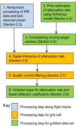
Figure 2.Flow diagram for the components of the radar algorithm.
the attenuation rate (Sect. 2.4) uses the framework developed by MacGregor et al. (2007, 2015b) and assumes temperature fields from the GISM (Greenland Ice Sheet Model)
(Huy-brechts, 1996; Shapiro and Ritzwoller, 2004; Goelzer et al., 2013), and SICOPOLIS (SImulation COde for POLythermal Ice Sheets) (Greve, 1997) thermomechanical models. The Arrhenius model is used to firstly constrain the sample re-gion for the algorithm (Sect. 2.5), then to correct for local attenuation variation within each region when inferring the attenuation rate (Sect. 2.6). Sections 2.5 and 2.6 represent the central original method contributions in this study. They both address how the regional bed-returned power method for attenuation evaluation (which assumes local constancy) can be modified for spatial variation. Algorithm quality con-trol is then implemented by testing for regions where the at-tenuation solution is marked by strong correlation between bed-returned power and ice thickness (Sect. 2.7). Finally, maps are produced for the radar-inferred attenuation rate, the two-way attenuation loss, and the basal reflection coef-ficient (Sect. 2.8). A list of principle symbols is provided in Table A1 in Appendix A.
2.3 Waveform processing
principles, the aggregated definition of bed-returned power for a diffuse surface is more directly related to the predicted (specular) reflection coefficients than equivalent peak power values (Oswald and Gogineni, 2008). In our study we make two important modifications to this method, which are de-scribed here, along with an overview of the key processing steps. The first modification corresponds to defining a vari-able window size for the along-track averaging of the basal waveform (which enables us to optimise the effective data resolution in thin ice), and the second corresponds to the im-plementation of an automated waveform quality control pro-cedure.
Using the waveform processing method of Oswald and Gogineni (2008, 2012), the along-track waveform averaging window is set using the first return radius
r= s
p
s+√h ǫice
, (1)
where p=4.99 m is the (prewindowed) radar pulse half-width in air (Rodriguez-Morales et al., 2014),sis the height of the radar sounder above the ice surface,his the ice thick-ness, andǫice=3.15 is the real part of the relative dielectric permittivity for ice. A flat surface,r corresponds to the ra-dius of the circular region illuminated by the radar pulse such that it extends the initial echo return by<50 % (Oswald and Gogineni, 2008). Additionally, if adjacent waveforms within this region are stacked about their initial returns and arith-metically averaged, they represent a phase-incoherent aver-age where the effects of power fluctuations due to interfer-ence are smoothed (Oswald and Gogineni, 2008; Peters et al., 2005). Oswald and Gogineni (2008, 2012) considered the northern interior of the GrIS where h∼3000 m, and sub-sequentlyr and the along-track averaging interval were ap-proximated as being constant. Since our study considers IPR data from both the ice margins and the interior, we use Eq. (1) to define a variable size along-track averaging window. For the typical flying height ofs=480 m,rranges from∼55 m in thin ice (h=200 m) to∼105 m in thick ice (h=3000 m), though can be higher during plane manoeuvres. The number of waveforms in each averaging window is then obtained by dividing 2rby the along-track resolution.
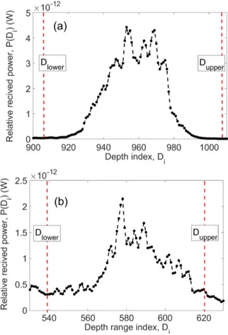
The incoherently averaged basal waveforms range from sharp pulse-like returns associated with specular reflection, to broader peaks associated with diffuse reflection (refer to Oswald and Gogineni, 2008 for a full discussion). An ex-ample of an incoherently averaged waveform is shown in Fig. 3a, in units of linear power, P, vs. depth-range index
Di. The plot shows the upper and lower limits of the power
depth integral,DlowerandDupper. These limits are symmet-ric about the peak power value, with(Dupper−Dlower)=2r (in units of the depth-range index); a range motivated by the observed fading intervals described in Oswald and Gogineni (2008). Subsequently, as is the case for the along-track av-eraging bin, the power integral limits vary over the extent of
Figure 3. Waveform processing using the power depth integral method, Eq. (2). (a) A waveform that satisfies the quality con-trol criteria (decays to 2 % of peak power within integral bounds). (b)A waveform that does not satisfy the quality control criteria.
the ice sheet and are of greater range in thicker ice. The ag-gregated (integrated) power is then defined by
Pagg=
Di=Dupper X
Di=Dlower
P (Di). (2)
Waveform quality control was implemented by testing if the waveform decayed to a specified fraction of the peak power value within the integral limitsDlower andDupper. This ef-fectively tests whether the SAR beamwidth is large enough to include all of the scattered energy, which was argued to be the general case by Oswald and Gogineni (2008). Decay fractions of 1, 2, and 5 % were considered, and 2 % was es-tablished to give the best coverage, whilst excluding obvious waveform anomalies. The waveform in Fig. 3a is an example that satisfies the quality control measure, whereas the wave-form shown in Fig. 3b does not. The relative decibel power for each waveform is then defined by
[P] =10log10Pagg, (3)
spreading using
[PC] = [P] − [G], (4)
where
[G] =20 log10 gλ0 8πs+√hǫ
ice
, (5)
(Bogorodsky et al., 1983b) withg=4 the antenna gain (cor-responding to 11.8 dBi) (Paden, 2015), andλ0=1.54 m the central wavelength of the radar pulse (Rodriguez-Morales et al., 2014).
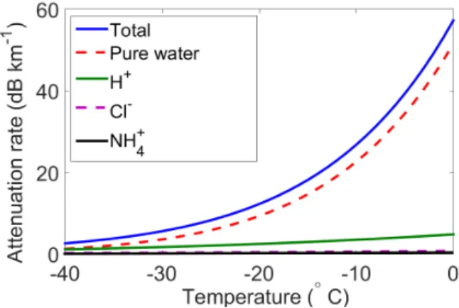
2.4 Arrhenius temperature model for attenuation It is well established that the dielectric conductivity and radar attenuation rate in glacier ice is described by an Ar-rhenius relationship where there is exponential dependence upon inverse temperature and a linear dependence upon the concentration of soluble ionic impurities (Corr et al., 1993; MacGregor et al., 2007, 2015b; Stillman et al., 2013). The Arrhenius modelling framework introduced by MacGre-gor et al. (2015b) for the GrIS, which we adopt here, in-cludes three soluble ionic impurities: hydrogen/acidity (H+), chlorine/sea salt (Cl−), and ammonium (NH+4). Our Arrhe-nius model assumes uniform, depth-averaged, molar concen-trations: cH+=0.8 µM, cCl−=1.0 µM and cNH+
4 =0.4 µM (M=mol L−1), which are derived from GRIP core data (MacGregor et al., 2015b). A decomposition of the temper-ature dependence for the attenuation rate for pure ice and the different ionic species is shown in Fig. 4. Use of layer stratigraphy for the concentration of the ionic species (rather than depth-averaged values) is discussed in detail in MacGre-gor et al. (2012, 2015b). The equations and parameters for the model calculation of the attenuation rate, Bˆ (dB km−1), the depth-averaged attenuation rate,<B >ˆ (dB km−1), and the two-way attenuation loss [ ˆL](dB) are outlined in Ap-pendix B. Throughout this manuscript we use Xˆ notation to distinguish Arrhenius model estimates from the radar-derived values and < X > to indicate dept averages. For brevity we often refer to the depth-averaged attenuation rate as the attenuation rate.
The Arrhenius relationship is empirical and the dielectric properties of impure glacier ice (pure ice conductivity, mo-lar conductivities of soluble ionic impurities, and activation energies) need to be measured with respect to a reference temperature and frequency. Two Arrhenius models for the di-electric conductivity and the attenuation rate were applied to the GrIS by MacGregor et al. (2015b): the W97 model intro-duced by Wolff et al. (1997), and the M07 model introintro-duced by MacGregor et al. (2007). For equivalent temperature and chemistry the W97 model produces conductivity/attenuation rate values at ∼65 % of the M07 model (MacGregor et al., 2015b). In Appendix B we describe these models in more detail, along with an empirical correction to the W97 model
Figure 4.Temperature dependence of estimated attenuation rate, ˆ
B, assuming depth-averaged chemical concentrations at GRIP core and the Arrhenius model, M07, in MacGregor et al. (2007).
(hereafter referred to as W97C), which accounts for a pro-posed frequency dependence of the dielectric conductivity between the radar system frequency (195 MHz) and the ref-erence frequency of the Arrhenius model (300 kHz). In Ap-pendix A we propose a test, based upon the thickness cor-relation for the estimated values of the basal reflection co-efficient, for how well tuned each model is for estimating the conductivity/attenuation at the radar frequency. From this test we conclude that the M07 model provides a suitable es-timate for our algorithm, and unless stated we use it in all further attenuation estimates.
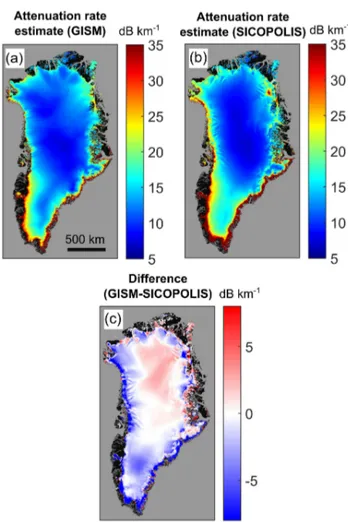
The temperature fields for GISM and SICOPOLIS were used to estimate the spatial variation in the depth-averaged attenuation rate for the GrIS and were interpolated at 1 km grid resolution. Both the GISM and SICOPOLIS models provide temperature profiles as a function of relative depth, and these were vertically scaled using the 1 km Greenland Bedmap 2013 ice thickness data product (Bamber et al., 2013). For the SICOPOLIS temperature field it is neces-sary to convert the (homologous) temperature values from degrees below pressure melting point to units of K (or◦C) using a depth correction factor of−0.87 K km−1(Price et al., 2015). For both temperature fields, the attenuation rate is predicted to vary extensively over the GrIS, with minimum values in the interior (∼7 dB km−1) and maximum values for the south-western margins of>35 dB km−1(shown for GISM in Fig. 5a and SICOPOLIS in Fig. 5b). Toward the ice sheet margins GISM generally has a lower temperature and therefore a lower attenuation rate than SICOPOLIS (Fig. 5c). The GISM vertical temperature profiles are in better overall agreement with the temperature profiles at the deep ice core sites shown in Fig. 1b (refer to MacGregor et al., 2015b for summary plots of the core temperature profiles).
2.5 Constraining the algorithm sample region
thick-Figure 5. Estimated spatial dependence of depth-averaged atten-uation rate for the GrIS using the Arrhenius model. (a) GISM temperature field, <B(Tˆ GISM) >. (b) SICOPOLIS temperature
field,<B(Tˆ SIC) >.(c)Attenuation rate difference plot for
GISM-SICOPOLIS,<B(Tˆ GISM) >−<B(Tˆ SIC) >.
ness, requires sampling IPR data from a local region of the ice sheet (Gades et al., 2000; MacGregor et al., 2007; Jacobel et al., 2009; Fujita et al., 2012; Matsuoka et al., 2012b). An implicit assumption of the method is that the depth-averaged attenuation rate is constant across the sample region (Lay-berry and Bamber, 2001; Matsuoka et al., 2010a). However, as was shown in Sect. 2.4, the depth-averaged attenuation rate is predicted to have pronounced spatial variation, and therefore an ice-sheet-wide radar attenuation algorithm must take this into account. In our development of an automated framework we use the spatial distribution of<B >ˆ (the prior Arrhenius model estimate) to constrain the size and shape of the sample region as a function of position (a “moving target window”) by estimating regions where the attenuation rate is constant subject to a specified tolerance. The most gen-eral, but computationally expensive, approach to defining the sample region would be to define an irregular contiguous re-gion about each window centre where the attenuation rate is less than a tolerance criteria (such as an absolute
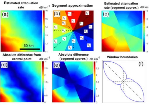
differ-ence). Here, motivated by computational efficiency, we have developed a “segmentation approximation” for defining the anisotropic sample region window. This approach uses local differences in the estimated<B >ˆ field along eight grid di-rections, and is similar in its representation of anisotropy to numerical gradient operators defined on an orthogonal grid. Below we describe the key conceptual steps to our method with the further details in Appendix C.
Figure 6a illustrates an example of the anisotropy that can occur in the spatial distribution of <B >ˆ for a 120 km2 region of the GrIS. The target window is divided into eight segments (notated by Sn with n=1,2, . . .,8), in a
plane-polar coordinate system about a central point (x0,y0) (Fig. 6b) with the ultimate goal to produce a variable ra-dial length of the target window by interpolating with re-spect to angle. The size of each segment is defined by its central radius vector, Rn, for angles θn=(n−81)π, with
R1=R5,R2=R6,R3=R7,R4=R8. The estimate<B >ˆ is then approximated in the plane-polar coordinate system by defining the attenuation rate in each segment to have the same radial dependence as along the direction of the central radius vector: <B(r) >ˆ =<B(rˆ n, θn) > with r=
p
(x−x0)2+(y−y0)2(Fig. 6c). The Euclidean distance of
<B >ˆ from (x0,y0) is then used to define a tolerance metric, shown for
q
(<B(x, y) >ˆ −<B(xˆ 0, y0) > )2 in Fig. 6d and
q
(< B(rˆ n, θn) >−<B(xˆ 0, y0) > )2(the segment ap-proximation) in Fig. 6e. Finally, the boundaries of the tar-get window are defined by linear interpolation along a circu-lar arc (Fig. 6f). Note that the target window boundaries are largest in the direction approximately parallel to the contours of constant<B >ˆ in Fig. 6a.
A primary consideration for the moving target window is that the dimensions,Rn, are smoothly varying in space. If the
converse were true then there would be a sharp discontinu-ity in the IPR data that is sampled. It was established that, rather than use of a simple maximum Euclidean distance cri-teria to defineRn, a root mean square (rms) integral
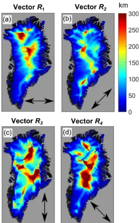
mea-sure produces greater spatial continuity (described fully in Appendix C). The spatial distribution of the target window radius vectorsR1,R2,R3,R4using GISM temperature field are shown in Fig. 7. All four plots have the general trend that the target window radii are larger in the interior of the ice sheet corresponding to where the <B >ˆ field is more slowly varying. The dependence ofR1,R2,R3,R4upon the anisotropy of the<B >ˆ field in Fig. 5 is also evident, with larger radii approximately parallel to contours of constant
Figure 6. Constraining the target window boundaries. (a) Estimated attenuation rate, <B(x, y) >ˆ . (b) Segment approximation: seg-ments Sn=1, . . .,7,8, radii Rn=1, . . .,7,8 with n=1, . . .,7,8. (c) Segment approximation for the attenuation rate, <B(r)>ˆ =<
ˆ
B(rn, θn) >. (d) Local tolerance/absolute difference,
q
(<B(x, y) >ˆ −<B(xˆ 0, y0) > )2. (e) Segment approximation for tolerance, q
(<B(rˆ n, θn) >−<B(xˆ 0, y0) > )2.(f)Target window boundaries.
gradient of depth-averaged temperature). Hence systematic biases in the model temperature fields are less important. 2.6 Radar inference of attenuation rate
The method of using the relationship between ice thickness and bed-returned power to infer the radar attenuation rate and basal reflection coefficient has been employed many times to local regions of ice sheets (Gades et al., 2000; Winebrenner et al., 2003; MacGregor et al., 2007; Jacobel et al., 2009; Fu-jita et al., 2012). An explanation for how this method works begins with the radar power equation
[PC] = [R] − [L], (6)
where [R]is the basal reflection coefficient, [L] is the to-tal (two way) power loss (Matsuoka et al., 2010a). This ver-sion of the radar power equation neglects instrumental fac-tors, which here we assume to be a constant for each field campaign. In our study[PC]is the aggregated geometrically corrected power, as defined by Eqs. (2)–(4), whereas in the majority of other studies[PC]is the geometrically corrected peak power of the basal echo. Equation (6) does not include additional loss due to internal scattering, which can occur when the glacial ice has crevasses and is not well stratified as is often the case for fast-flowing regions near the ice sheet margin (Matsuoka et al., 2010a; MacGregor et al., 2007). Expressing the total loss in terms of the depth averaged at-tenuation rate as[L] =2< B > h, and then considering the
variation in Eq. (6) with respect to ice thickness gives
δ[PC]
δh =
δ[R]
δh −2< B >, (7)
(Matsuoka et al., 2010a). If δ[δhR]≪δ[PδhC] (refer to Sect. 2.7
for the algorithm quality control measures that test for this), then
< B >≈ −1
2
δ[PC]
δh . (8)
Subsequently, radar inference of the attenuation rate is achieved via linear regression of Eq. (8), the total loss can be calculated from[L] =2< B > h, and the basal reflec-tion coefficients can be calculated from Eq. (6).
As discussed here and in Sect. 2.5, in applying this linear regression approach, it is assumed that the regression gra-dient (i.e. the depth-averaged attenuation rate) is constant throughout the sample region, which can lead to erroneous slope estimates (Matsuoka, 2011). In practice, however, the sample region must necessarily include ice with a range of thicknesses, and therefore a range of temperatures and at-tenuation rates. In our modification to the basic method, the Arrhenius model is used to “standardise” bed-returned power for local attenuation variation, using the central point of each target window as a reference point. This is achieved via the power correction
[PC]i→ [PC]i+2
<B(xˆ i, yi) >−<B(xˆ 0, y0) >
Figure 7. Maps for target window radii vector length using the GISM temperature field.(a)VectorR1,(b)VectorR2,(c)Vector
R3,(d)VectorR4. The orientation of each radii vector is shown in
each subplot.
where(xi, yi)corresponds to the position of theith data point
within the target window and(x0, y0)corresponds to the cen-tral point. This power correction represents an estimate of the difference in attenuation loss between an ice column of the actual measurement (loss estimate 2<B(xˆ i, yi) > hi), and a
hypothetical ice column with the same thickness as the mea-surement but with the attenuation rate of the central point (loss estimate 2<B(xˆ 0, y0) > hi).
An example of a[PC]vs.hregression plot pre- and post-power correction, Eq. (9), is shown in Fig. 8. In this exam-ple, ice columns that are thinner than the central point have
(<B(xˆ i, yi) >−<B(xˆ 0, y0) >) >0 and the power values are increased by Eq. (9), whereas ice columns that are thicker than the central point have(<B(xˆ i, yi) >−<B(xˆ 0, y0) >
) <0 and the power values are decreased. Subsequently, the power correction acts to enhance the linear correlation be-tween power and ice thickness (as demonstrated by the in-crease in ther2value in Fig. 8), and enables the underlying attenuation trend to be better discriminated. It follows that, for this situation described, failing to take into account the spatial variation in attenuation rate in the linear regression procedure results in a systematic underestimation of the at-tenuation rate. The difference in radar-inferred atat-tenuation
Figure 8. Bed-returned power vs. ice thickness pre- and post-local attenuation correction, Eq. (9). The radar-inferred attenuation rate pre correction is< B >=15.4 dB km−1(r2=0.56) and post-correction is< B >=19.3 dB km−1(r2=0.89). The central point of the sample region is 64.30◦N, 43.82◦W (100 km due south of the Dye 3 ice core) and has ice thickness 1604 m, and target window radii vectors:R1=39 km,R2=55 km,R3=108 km,R4=45 km.
rate pre- and post-power correction depends upon the dis-tribution of IPR flight track coverage within the sample re-gion and the size of the sample rere-gion, and is typically∼1– 4 dB km−1. Equation (9) represents our central modification to the bed-returned power method for deriving attenuation. We anticipate that, if a temperature model is available, this correction for local attenuation variation could be applied in future regional studies (even if the windowing methods de-scribe in Sect. 2.5 are not).
When applying the linear regression approach described in this section, IPR data from each field season were consid-ered separately. To ensure that there were sufficiently dense data within each sample region, a minimum threshold of 20 measurements was enforced, where each measurement cor-responds to a separate along-track averaged waveform as de-scribed in Sect. 2.3. Additionally, target window centres that were more than 50 km from the nearest IPR data point were excluded.
2.7 Quality control
The accuracy of the radar-inferred attenuation rate solution from Eq. (8) depends upon (i) a strong correlation between bed-returned power and ice thickness,δ[δhPC], (ii) a weak cor-relation between reflectivity and ice thickness, δ[δhR], relative toδ[δhPC]. To make a prior estimate of the correlation for δ[δhR] we use the prior Arrhenius model estimate of the basal re-flection coefficient governed by
and consider the correlation and linear regression model for
δ[ ˆR]
δh . The joint quality control threshold as follows:
r2
[PC] > α (11)
rratio2 = r2
[PC]
r2
[PC]+r2 [ ˆR]
> β, (12)
is then enforced wherer2
[PC]andr2 [ ˆR]arer
2correlation co-efficients for the δ[PδhC] and δ[ ˆδhR] linear regression models, and 0≥α≥1, 0≥β≥1 are threshold parameters. The first thresholding criteria, Eq. (11), tests for strong absolute corre-lation inδ[PδhC], and the second thresholding criteria, Eq. (12), tests for strong relative correlation in δ[δhPC] with respect to
δ[ ˆR]
δh . The name for ther
2
ratioparameter indicates that it is the “correlation ratio”. Both quality measures are designed with attenuation rate/loss accuracy in mind (rather than directly constraining the distribution of relative reflection). Unlike the use of the Arrhenius model attenuation estimate in Sects. 2.5 and 2.6, which uses the local difference in the<B >ˆ field, in Eq. (10) the absolute value of<B >ˆ is used. A justification for the use of the absolute value here is that it is used only as a quality control measure and does not directly enter the calculation of the radar-inferred attenuation rate.
In general, r2
[ ˆR]can be high (or equivalentlyr
2
ratiocan be low) due to (i) there being a true correlation in the basal re-flection coefficient with thickness, (ii) there being a correla-tion due to addicorrela-tional losses other than attenuacorrela-tion such as internal scattering, and (iii) the Arrhenius model estimate of the attenuation rate being significantly different from the true attenuation rate. Whilst the first two reasons are both desir-able for quality control filtering, the third reason is an erro-neous effect. However, as the dual threshold filters out all three classes of sample region, this erroneous effect simply reduces the coverage of the algorithm.
2.8 Gridded maps
The attenuation rate solution from the radar algorithm, < B >, is at a 1 km grid resolution and arises as a consequence of the scan resolution of the moving target window described in Sect. 2.5. It is defined on the same polar-stereographic co-ordinate system as in Fig. 1 and the gridded thickness data from Bamber et al. (2013). Subsequently, a gridded data set for the two-way loss can be calculated using[L] =2< B > h. For grid cells that contain IPR data, the mean[PC]value is calculated and, using Eq. (6), an along-track map for the grid-ded relative reflection coefficient,[R], is obtained. Due to the definition of relative power in Eqs. (3) and (4), the values of [R]are also relative. As described in Sect. 2.3 the averaging procedure for the basal waveforms means that the effective resolution of the processed IPR data varies over the extent of the ice sheet. Consequently, the number of data points that
are arithmetically averaged in each grid cell varies accord-ing to both this resolution variation and the orientation of the flight tracks relative to the coordinate system. For a single flight line (i.e. no intersecting flight tracks), the number of points in a grid cell typically ranges from∼4 in thick ice to ∼16 in thin ice. Initially, maps for the four field seasons were independently processed, which enables crossover analysis for the uncertainty estimates. Joint maps were then produced by averaging values where there were grid cells with cover-age overlap.
3 Results and discussion
With a view toward identifying regions of the GrIS where the radar attenuation algorithm can be applied, we firstly con-sider ice-sheet-wide properties for the linear regression cor-relation parameters (Sect. 3.1). We then demonstrate that, on the scale of a major drainage basin, basin 4 in Fig. 1b (SE Greenland), the attenuation solution converges for the two input temperature fields (Sect. 3.2). We go on to show that the converged attenuation solution produces a physically re-alistic range and spatial distribution for the basal reflection coefficient (Sect. 3.3). The relationship between algorithm coverage and uncertainty is then outlined (Sect. 3.4). Finally, we consider how the attenuation solution can be used to pre-dict temperature bias in thermomechanical ice sheet models (Sect. 3.5).
3.1 Ice-sheet-wide properties
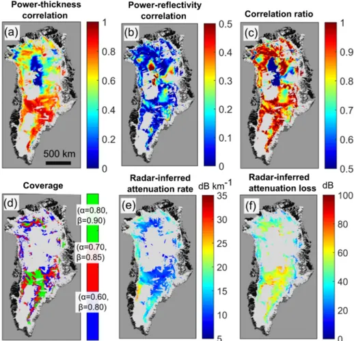
Ice-sheet-wide maps for the linear regression correlation pa-rameters are shown in Fig. 9a–c using the GISM tempera-ture field as an input. As discussed in Sects. 2.6 and 2.7, the radar algorithm requires (i) a strong correlation between bed-returned power and ice thickness (highr2
[PC]), (ii) a weak correlation between basal reflection and ice thickness (low
r2
[ ˆR]and highr
2
ratio). In general,r[2PC]has stronger correlation values in southern Greenland (typically ∼0.7–0.9). These regions of higher correlation correspond to where there is higher variation in ice thickness due to basal topography, and are correlated with regions of higher topographic roughness (Rippin, 2013). Correspondingly, in the northern interior of the ice sheet, where the topographic roughness is lower, there are weaker correlation values forr2
[PC](typically∼0.2–0.3). The correlation values forr2
[PC] in the northern interior can also, in part, be explained by the lower absolute values for the depth-averaged attenuation rate as predicted in Fig. 5. The correlation values forr2
[ ˆR]are generally much lower than
r2
[PC]and more localised. As discussed in Sect. 2.7, regions wherer2
[ ˆR]is high can arise due to both true target-window
scale variation in the basal reflector or due to a significant bias in the Arrhenius model estimation,[ ˆR]. The values for
rratio2 , are largely correlated withr2
Figure 9.Ice-sheet-wide properties of the radar algorithm using the GISM temperature field.(a)Power–thickness correlation,r2
[PC].(b)
Ar-rhenius reflection coefficient-thickness correlation,r2
[ ˆR].(c)Correlation ratio,r 2
ratio, Eq. (12).(d)Coverage for three thresholds (green is a
subset of red and red is a subset of blue). (e) Radar-inferred attenuation rate,< B(TGISM) >, for(α, β)=(0.60,0.80).(f)Radar-inferred
attenuation loss,[L(TGISM)], for(α, β)=(0.60,0.80).
Examples of algorithm coverage for three different sets of (α,β) quality control thresholds, Eqs. (11) and (12), are shown in Fig. 9d. These are chosen such that each succes-sively higher quality threshold region is contained within the lower threshold region. In Sect. 3.4 we discuss how the cov-erage regions relate to uncertainty in the radar-inferred at-tenuation rate and two-way atat-tenuation loss, and the central problem of the radar inference of the basal material proper-ties. For the discussion here, it is simply important to note that algorithm coverage is fairly continuous for a significant proportion of the southern ice sheet (corresponding to large regions of major drainage basins 4–7) and toward the mar-gins of the other drainage basins. The spatial distribution of the radar-inferred attenuation rate,< B(TGISM) >, is shown in Fig. 9e and the radar-inferred attenuation loss,[L(TGISM)], is shown in Fig. 9f, both of which are for the threshold
(α, β)=(0.6,0.8). Note that the ice-sheet-wide properties for< B(TGISM) >are similar to the Arrhenius model predic-tions (Fig. 5a) with higher values (∼15–30 dB km−1) toward
the ice margins and lower values (∼7–10 dB km−1) in the interior.
The ice-sheet-wide properties of the algorithm are pre-served using the SICOPOLIS temperature field as an input (refer to Supplement for a repeat plot of Fig. 9). Notably, the ice-sheet-wide distribution forr2
[PC]is similar, and for equiv-alent choices of threshold parameters there is better coverage for the southern GrIS than for the northern interior.
3.2 Attenuation solution convergence
To demonstrate the convergence of the attenuation solution for different input temperature fields (convergence is de-fined here as a normally distributed difference distribution about zero), we compare the solution differences for the (input) Arrhenius models, <B(Tˆ GISM) >−<B(Tˆ SIC) > and [ ˆL(TGISM)] − [ ˆL(TSIC)], with the corresponding (out-put) radar-inferred solution differences,< B(TGISM) >−<
B(TSIC) >and[L(TGISM)] − [L(TSIC)]. As[L] =2< B >
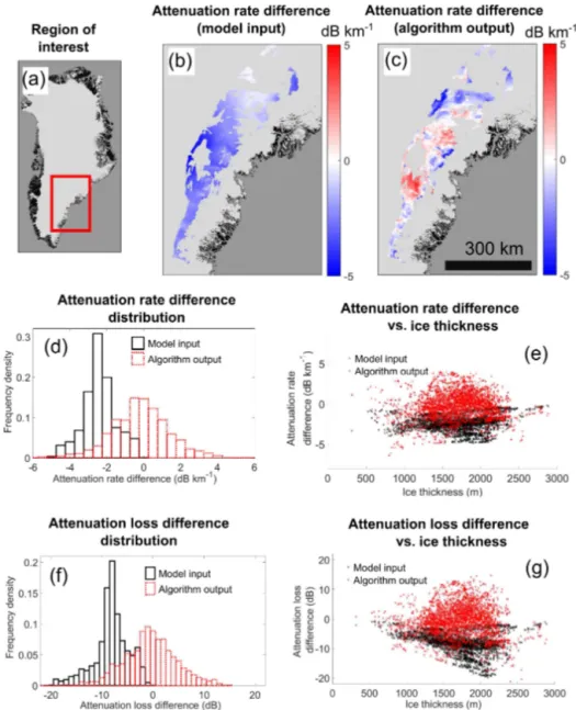
Figure 10.Attenuation solution convergence for the SE GrIS.(a)Region of interest.(b)Map for<B(Tˆ GISM) >−<B(Tˆ SIC) >(Arrhenius
model input).(c)Map for< B(TGISM) >−< B(TSIC) >(algorithm output).(d)Difference distributions for(b)and (c). (e) Thickness
dependence for plot(d).(f)Difference distributions for attenuation loss.(g)Thickness dependence for plot(f).
solution differences and the consequences for a thickness-correlated bias in basal reflection values. We focus on the south-east GrIS, corresponding to target window centres that are located in drainage basin 4 Fig. 1a. This region is se-lected post-ice-sheet-wide processing, and the IPR data from neighbouring drainage basins are incorporated in the linear regression plots for the target windows that lie close to the basin boundaries. We consider an attenuation rate solution for fixed threshold parameters(α, β)=(0.6,0.8). These are chosen to achieve a solution uncertainty deemed to approach the accuracy required to discriminate basal melt (discussed fully in Sect. 3.4).
The inset region we consider is shown in (Fig. 10a). The prior Arrhenius model solution difference for the attenuation
rate, <B(Tˆ GISM) >−<B(Tˆ SIC) >, is strongly negatively biased (Fig. 10b). If the solution difference is aggregated over all grid cells that contain IPR data, the mean and standard deviation,µ±σ, is−2.42±0.88 dB km−1(Fig. 10d). Note thatσ does not represent an uncertainty for the Arrhenius-modelled attenuation rate. It is a measure of the spread of the two different input attenuation rate fields. On the scale of the drainage basin, this solution bias is approxi-mately constant with ice thickness (Fig. 10e). By contrast, the radar algorithm solution difference,<B(Tˆ GISM) >−<
ˆ
zero,µ±σ = −0.18±1.53 dB km−1(Fig. 10d), and approx-imately constant with ice thickness (Fig. 10e).
Corresponding difference distributions for the attenuation loss are shown in Fig. 10f and g. These represent a rescal-ing of the distributions in Fig. 10d and e by the factor 2h
and do not take thickness uncertainty into account. The Ar-rhenius model solution difference is weakly negatively corre-lated with thickness (r2=0.09), and from Eq. (6) results in a thickness-correlated bias for the basal reflection coefficient. As the attenuation loss solution bias can be>10 dB for thick ice (h∼2000 m or greater), this would potentially result in a different diagnosis of thawed and dry glacier beds using the different temperate fields in the Arrhenius model. Again, the radar-inferred solution difference is approximately nor-mally distributed about zero (µ±σ= −0.56±5.19 dB). The radar-inferred difference is also uncorrelated with ice thick-ness (r2=0.00), which is highly desirable for unambiguous radar inference of basal material properties on an ice-sheet-wide scale.
If a similar analysis for the attenuation solution differences is applied to drainage basins 3, 5, and 6 (southern and east-ern Greenland) we observe algorithm solution convergence (in the sense of a normally distributed difference centred on zero) and an associated reduction in the solution bias from the Arrhenius model input. In drainage basins 1, 2, 7, and 8 (northern and western Greenland), we do not observe analo-gous solution convergence for the radar-inferred values. We do, however, typically see a reduction in the mean system-atic bias for the attenuation rate/loss solution relative to the Arrhenius model input. In the Supplement we provide ad-ditional plots and discuss the potential reasons for the algo-rithm non-convergence, which are thought to relate primarily to the more pronounced temperature sensitivity of the algo-rithm target windows in the northern GrIS.
3.3 Attenuation rate and basal reflection maps
For regions of the GrIS where the attenuation rate solution converges and there is algorithm coverage overlap for the different temperature field inputs, it is possible to define the mean radar-inferred attenuation rate solution
< B>=1
2(< B(TSIC) >+< B(TGISM) >) . (13) Note that the explicit temperature dependence for the mean value is dropped as, for the regions of convergence, it rep-resents a solution that is (approximately) independent of the input temperature field. Within the drainage basins where the solution converges and where only one of < B(TSIC) >or
< B(TGISM) >is above the coverage threshold, we use the single values to define the mean < B >field. A justifica-tion for this approach is that a region where only one tem-perature field has coverage is most likely to be an instance of where the other temperature field has erroneous estimates for δδh[ ˆR] as discussed in Sect. 2.7. Hence, for a given(α, β)
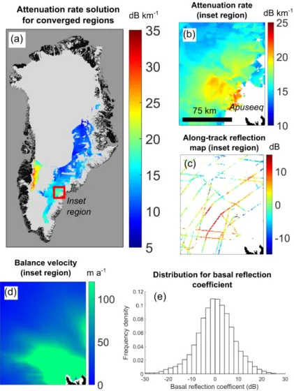
threshold, the coverage region for< B >is slightly larger than for < B(TSIC) > and < B(TGISM) >. A map for the converged attenuation rate solution using Eq. (13) is shown in Fig. 11 for coverage threshold(α, β)=(0.60,0.80). This field is generally smoothly varying, as would be expected given its primary dependence upon temperature.
Inset maps for the depth-averaged attenuation rate and basal reflection coefficient are compared with balance veloc-ity (Bamber et al., 2000) in Fig. 11b–d. Following the nam-ing convention in Bjørk et al. (2015), this region is upstream from the Apuseeq outlet glacier. Balance velocities rather than velocity measurements are used due to incomplete ob-servations in the region of interest (Joughin et al., 2010). The correspondence between the fast-flowing region (ap-proximately >120 m a−1) and the near-continuous regions of higher attenuation rate (approximately>18 dB km−1) and higher basal reflection values (approximately>8 dB) is evi-dent. This supports the view that the fast-flowing region cor-responds to relatively warm ice, and is underlain by a pre-dominately thawed bed which acts to enhance basal sliding.
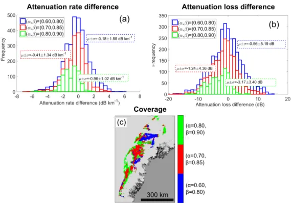
The probability distribution for the relative basal reflec-tion coefficient,[R], over the converged region is shown in Fig. 11e. The distribution is self-normalised by setting the mean value to equal zero. The decibel range is∼20 dB which is consistent with the predicted decibel range for subglacial materials (Bogorodsky et al., 1983a), and our estimate of the loss uncertainty (∼5 dB), discussed in more detail in Sect. 3.4. Since our definition of the basal reflection coef-ficient is based upon the aggregated definition of the bed-returned power, Eqs. (2) and (3), the overall range will be less than using the conventional peak power definition. 3.4 Relationship between uncertainty and coverage There are two metrics, both as a function of the quality threshold parameters(α, β), that we propose can be used to quantify the uncertainty of the radar algorithm. The first met-ric is the standard deviation of the attenuation solution dif-ferences for different input temperature fields as previously described in Sect. 3.2. This metric assesses solution varia-tion due to the target windowing and the local correcvaria-tion to the power within the target window described in Sects. 2.5 and 2.6 respectively. The second metric is to consider the standard deviation of the attenuation solution differences for independently analysed field seasons for a fixed input temperature field. This metric tests whether the waveform-processing and system performance are consistent between different field seasons. Furthermore, it tests whether differ-ent flight track distributions and densities in the same target window produce a similar radar-inferred attenuation rate.
Figure 11.Attenuation solution and basal reflection.(a)Converged radar-inferred attenuation rate map,< B >(average for both input temperature fields).(b)Attenuation rate map for inset region.(c)Along-track map for basal reflection coefficient for inset region.(d)Balance velocities for inset region. (e) Probability distribution for basal reflection coefficient for entire coverage region in(a). The reflection coefficient is defined using the aggregated power for the basal echo.
for grid cells that contain IPR data within drainage basin 4. It is clear that the standard deviation of the difference dis-tribution is related to how strict the coverage threshold is, with the strictest coverage threshold having the smallest stan-dard deviation value (refer to plots for values). Subsequently, we suggest that the coverage of the algorithm is a trade-off with uncertainty. The systematic bias for the strictest cover-age threshold, (α, β)=(0.80,0.90), is thought to arise due to sampling an insufficiently small region of the ice sheet. The standard deviation values in Fig. 12 for drainage basin 4 are similar in the other drainage basins where there is so-lution convergence. For example, for (α, β)=(0.60,0.80),
σ ∼1.5 dB km−1for the attenuation rate difference distribu-tion.
A similar relationship between the choice of(α, β) thresh-old parameters and solution accuracy arises for indepen-dently analysed field campaign data, and a full data
ta-ble is supplied in the Supplement. The attenuation solu-tion difference distribusolu-tions are close to being normally dis-tributed about zero, with small systematic biases (∼0.1– 0.7 dB km−1) for the attenuation rate. For the same choice of(α, β)threshold parameters, the attenuation rate solution standard deviations are of similar order to the equivalent temperature field difference distributions. For example, for
(α, β)=(0.60,0.80),σ is in the range 0.98–1.71 dB km−1 for the different field season pairs.
Figure 12.Relationship between algorithm coverage and uncertainty as measured by attenuation solution difference distributions.(a) Atten-uation rate,< B(TGISM) >−< B(TSIC) >.(b)Attenuation loss,[L(TGISM)] − [L(TSIC)].(c)Algorithm coverage. Green is a subset of red
and red is a subset of blue. The region is the same as Fig. 10.
a typical sample region (ice thickness∼1500–2000 m), it re-sults in a desired attenuation rate accuracy∼1–1.5 dB km−1. For both uncertainty metrics this corresponds to approxi-mately(α, β)=(0.6,0.8). This interpretation of uncertainty is consistent with the∼20 dB range for the basal reflection coefficients in Fig. 11. Throughout the algorithm develop-ment, we continually considered both uncertainty metrics. Of particular note, if the Arrhenius model is used to constrain the target window dimensions (Sect. 2.5), but not to make a power correction within each target window (Sect. 2.6), there are more pronounced systematic biases present for both un-certainty metrics.
The recent study by MacGregor et al. (2015b) also pro-duced a GrIS wide map for the radar-inferred attenuation rate. This study used returned power from internal layers in the glacier ice to infer the attenuation rate (Matsuoka et al., 2010b), and the values are therefore only for some fraction of the ice column (roughly corresponding to the isothermal region of the vertical temperature profiles). The uncertainty was quantified using the attenuation rate solu-tion standard deviasolu-tion (σ=3.2 dB km−1) at flight transect crossovers. A direct comparison between their uncertainty estimate and ours is not possible, as we use a different def-inition of crossover point (i.e. all grid cells that contain IPR data in a mutual coverage region), and we can tune the cov-erage of our algorithm for a desired solution accuracy. Addi-tionally, whereas each value using the internal layer method is spatially independent, the moving target-windowing
ap-proach of our algorithm means each radar-inferred value is dependent upon neighbouring estimates.
3.5 Evaluation of temperature bias of ice sheet models The evaluation of the temperature bias of a thermomechani-cal ice sheet model using attenuation rates inferred from IPR data was recently considered for the first time by MacGre-gor et al. (2015b); in this case the ISSM (Ice Sheet System Model) model described by Seroussi et al. (2013). For the internal layer method used by MacGregor et al. (2015b) the attenuation rate inferred from the IPR data represents a truly independent test of temperature bias. For our method, which uses ice sheet model temperature fields as an input, this is not necessarily the case, and we only consider regions where the radar-inferred values tend to converge for different input tem-perature fields (the map in Fig. 11a). The inversion of the Ar-rhenius relations (solving for a depth-averaged temperature given a depth-averaged attenuation rate) is both a non-linear and non-unique problem. We leave this problem, which is po-tentially more complex for the full ice column than the depth section where internal layers are present (which is closer to being isothermal), for future work. Instead we estimate tem-perature bias using the Arrhenius model radar algorithm so-lution differences for the Arrhenius model-radar algorithm:
Figure 13. Evaluation of temperature bias for ice sheet models using attenuation rate differences. (a) <B(Tˆ GISM) >−< B >:
M07. (b) <B(Tˆ SIC) >−< B >: M07. (c) <B(Tˆ GISM) >−<
B >: W97C (σ195 MHz/σ300 kHz=1.7). (d) <B(Tˆ SIC) >−<
B >: W97C (σ195 MHz/σ300 kHz=1.7). Red regions are suggestive
of positive bias for depth-averaged temperature and blue regions are suggestive of negative bias. (e) Temperature profiles at Dye 3 core. The model temperature profiles are vertically rescaled using the ice core thickness (2038 m), and the core temperature profile is from (Gundestrup and Hansen, 1984).
and will not hold exactly if ionic concentrations or the shape of the vertical temperature profiles differ substantially over the region. In order to illustrate the sensitivity of our results, and the evaluation of model temperature fields in general, to the choice of conductivity model, we use the W97C model alongside the M07 model.
Arrhenius model-radar algorithm attenuation solution dif-ferences are shown for the M07 model (GISM Fig. 13a, SICOPOLIS Fig. 13b) and W97C model (GISM Fig. 13c, SICOPOLIS Fig. 13d). The frequency correction parame-ter for W97C corresponds to σ195 MHz/σ300 kHz=1.7 (the ratio of the dielectric conductivity at the IPR system fre-quency relative to the reference frefre-quency of the Arrhenius model), and is described in detail in Appendix B. Dye 3 is the only ice core within the coverage region and the model and core temperature profiles are shown in Fig. 13e. For the M07 model <B(Tˆ GISM) >−< B > is negative in the re-gion of the Dye 3 core (suggestive of negative temperature bias), whereas<B(Tˆ SIC) >−< B >is positive (suggestive of positive temperature bias) which is in agreement with the known model temperature biases Fig. 13e. Arrhenius model attenuation rate values at the core are<B(Tˆ GISM) >= 12.8 dB km−1and<B(Tˆ SIC) >=16.7 dB km−1and the radar inferred value is< B >=15.8 dB km−1. The W97C model (which estimates attenuation rate values∼10–15 % higher than the M07 model) is also consistent with this attenu-ation rate/temperature bias hierarchy, with <B(Tˆ SIC) >= 18.7 dB km−1and<B(Tˆ GISM) >=14.3 dB km−1. It is also possible to use the ice core temperature profile at Dye 3 in the Arrhenius model to predict depth-averaged attenua-tion rate values. This gives<B(Tˆ CORE) >=13.9 dB km−1 for the M07 model and <B(Tˆ CORE) >=15.8 dB km−1 for the W97C model. These values are both consistent with the radar-inferred value subject to the original uncertainty esti-mate of the M07 model (∼5 dB km−1when the temperature field is known MacGregor et al., 2007).
A final caveat to our approach here is that it does not in-clude layer stratigraphy in the Arrhenius model. The anal-ysis in MacGregor et al. (2015b) predicts that, through-out the GrIS, radar-inferred temperatures that incorporate layer stratigraphy are generally systematically lower (corre-spondingly depth-averaged attenuation rates are systemati-cally higher). This deficit is predicted to be most pronounced in southern and western Greenland, due to the higher fraction of Holocene ice in these regions which has higher acidity than the depth-averaged values at GRIP (MacGregor et al., 2015a).
4 Conclusions
previ-ous regional versions of the algorithm (Gades et al., 2000; MacGregor et al., 2007; Jacobel et al., 2009; Fujita et al., 2012; Matsuoka et al., 2012b). These included using a wave-form processing procedure that is specifically tuned for the evaluation of bulk material properties, incorporating a prior Arrhenius model estimate for the spatial variation in attenu-ation to constrain the sample area, standardising the power within each sample area and introducing an automated qual-ity control approach based on the underlying radar equa-tion. We demonstrated regions of attenuation solution con-vergence for two different input temperature fields and for independently analysed field seasons. A feature of the algo-rithm is that the uncertainty, as measured by standard devi-ation of the attenudevi-ation solution difference distribution for different input temperature fields and separate field seasons, is tunable. Subsequently, we suggested that the algorithm could be used for the discrimination of bulk material prop-erties over selected regions of ice sheets. Notably, assuming a total loss uncertainty of∼5 dB to be approximately suffi-cient for basal melt discrimination, we demonstrated that, on the scale of a major drainage basin, the attenuation solution produces a physically realistic (∼20 dB) range for the basal reflection coefficient.
The converged radar algorithm attenuation solution pro-vides a means of assessing the bias of forward Arrhenius temperature models. Where temperature fields are poorly constrained, and where the algorithm has good coverage, we suggest that it is preferable to using a prior Arrhenius model calculation. With this in mind, the potential problems with using a forward Arrhenius model for attenuation were illus-trated (Sect. 3.2). Notably, we demonsillus-trated that even a small regional bias in attenuation rate (this could arise either due to temperature bias or due a systematic bias in the Arrhe-nius model parameters) leads to thickness-correlated errors in attenuation losses and therefore the basal reflection coeffi-cients. These thickness-correlated errors persist regardless of whether the regional bias is with respect to the “true” value or to another modelled value. We hypothesise that the algo-rithm convergence for different input temperature fields oc-curs because the local differences in the Arrhenius model at-tenuation rate field that are used as an algorithm input (i.e.
<B(x, y) >ˆ −<B(xˆ 0, y0) >) are more robust than the ab-solute values. This is broadly equivalent to saying that the horizontal gradients in the depth-averaged temperature field of the ice sheet models are more robust than the absolute val-ues of the depth-averaged temperature. Similarly, our use of local differences for the attenuation rate estimate is also ro-bust to systematic biases in the Arrhenius model.
We have yet to consider an explicit classification of the subglacial materials and quantification of regions of basal melting. In future work, we aim to combine IPR data from preceding CReSIS field campaigns to produce a gridded data product for basal reflection values and basal melt. It is antici-pated that, as outlined by Oswald and Gogineni (2008, 2012) and Schroeder et al. (2013), the specularity properties of the basal waveform, and how this relates to basal melt detection, could also be incorporated in this analysis. As the regions of algorithm coverage are sensitive to uncertainty, we suggest that these data products could have spatially varying uncer-tainty incorporated. Additionally, for the basal reflection and basal melt data sets, uncertainty in the measurements of[PC]
will have to be incorporated in the uncertainty estimate for [R]. Establishing a procedure for the interpolation of these data sets where either: (i) the algorithm coverage is poor due to low attenuation solution accuracy, or (ii) the IPR data are sparse, will form part of this framework. Regions of lower so-lution accuracy generally correspond to the interior of the ice sheet where spatial variation in the attenuation rate is much less pronounced (primarily the northern interior). Due to this lower spatial variability (and despite the caveats in the para-graph above), these regions could potentially have their basal reflection values derived by using a forward Arrhenius tem-perature model for the attenuation.
Appendix A: Principal notation
Table A1.List of principal symbols.
Symbol Units Description Equation(s)
[PC] dB Aggregated and geometrically corrected bed-returned power (2)–(5)
h km Thickness of ice column
ˆ
B dB km−1 Arrhenius model estimate for attenuation rate (B1), (B2) [ ˆL] dB Arrhenius model estimate for two-way attenuation loss (B3)
<B >ˆ dB km−1 Arrhenius model estimate for depth-averaged attenuation rate (B4) [ ˆR] dB Arrhenius model estimate for basal power reflection coefficient (10)
Rn km Radius vectors for sample regions withn=1,2,3,4
rms(Rn) dB km−1 Root mean square tolerance measure for sample regions (C2)
< B > dB km−1 Radar-inferred value for depth-averaged attenuation rate (8) [L] dB Radar-inferred value for two-way attenuation loss
[R] dB Radar-inferred value for basal power reflection coefficient
r2
[PC] r2correlation coefficient for[PC]vs.h
r2
[ ˆR] r
2correlation coefficient for[ ˆR]vs.h
rratio2 Correlation ratio ofr2
[PC]to (r 2 [PC]+r
2
[ ˆR]) (12)
α Quality control threshold forr2
[PC] (11)
Appendix B: Additional information for Arrhenius model
B1 Model equations
In ice, a low loss dielectric, the radar attenuation rate, Bˆ
(dB km−1), is linearly proportional to the high-frequency limit of the electrical conductivity, σ∞(µS m−1), following the relationship
ˆ
B= 10log10e
1000ǫ0c√ǫice
σ∞, (B1)
wherecis the vacuum speed of the radio wave (Winebrenner et al., 2003; MacGregor et al., 2012). Forǫice=3.15, as is assumed here,Bˆ =0.921σ∞. The Arrhenius relationship de-scribes the temperature dependence ofσ∞for ice with ionic impurities present and is given by
σ∞ =σpureexp E
pure
kB
1
Tr− 1
T
+µH+cH+exp
EH+ kB
1
Tr− 1
T
+µCl−cCl−exp
ECl− kB
1
Tr− 1
T
+µNH+
4cNH+4 exp (
ENH+ 4
kB
1
Tr− 1
T )
, (B2)
where T (K) is the temperature,Tr is a reference temper-ature,KB=1.38×10⁻²³J K−1 is the Boltzmann constant,
andcH+,cCl− andcNH+
4 are the molar concentrations of the chemical constituents (µM) (MacGregor et al., 2007, 2015b). The model parameters are summarised in tabular form by MacGregor et al. (2015b) for both the M07 model and W97 model.
Following the assumptions in Sect. 2.4 for the GrIS tem-perature field, ionic concentrations, and ice thickness data set, it is possible to obtain the spatial dependence of the at-tenuation rate,B(x, y, z)ˆ , where(x, y)are planar coordinates andzis the vertical coordinate. The two-way attenuation loss for a vertical column of ice,[ ˆL(x, y)](dB), is then obtained via the depth integral
[ ˆL] =2
h
Z
0 ˆ
B(z)dz. (B3)
Finally, the depth averaged (one-way) attenuation rate, < ˆ
B(x, y) >(dB km−1) is calculated from
<B>ˆ =[ ˆL]/2h. (B4)
B2 Frequency dependence and empirical correction Both the W97 model and the M07 model assume that the dielectric conductivity/attenuation rate is frequency indepen-dent between the medium frequency (MF), 0.3–3 MHz (the
range that the Arrhenius model parameters are measured), and the very high frequency (VHF), 30–300 MHz (the range encompassing the frequency of IPR systems) (MacGregor et al., 2015b). The W97 model is derived using the dielectric profiling method at GRIP core and is referenced to 300 kHz (Wolff et al., 1997), whereas the M07 model is derived from a synthesis of prior measurements and is not referenced to a specific frequency (MacGregor et al., 2007). The empirical frequency correction to the W97 model between the MF and VHF, W97C, was motivated by an inferred systematic under-estimation in the attenuation rate at the GrIS ice cores. This analysis was based upon using reflections from internal lay-ers to derive attenuation rate values and then inverting the Arrhenius relations to estimate englacial temperature. The frequency corrected model represents a departure from the classical (frequency independent) Debye model for dielec-tric relaxations under an alternating elecdielec-tric field. The physi-cal basis for the frequency dependence is related to the pres-ence of a log-normal distribution for the dielectric relaxations (Stillman et al., 2013).
For the MCoRDS system that is considered in this study and by MacGregor et al. (2015b), the empirical frequency correction toσ∞in Eq. (B2) is given by
σ∞−→ σ
195 MHz
σ300 kHz
σ∞, (B5)
where σ195 MHz/σ300 kHz is the ratio of the conductivity at the central frequency of the radar system to the W97 model frequency. A ratio σ195 MHz/σ300 kHz=2.6 was in-ferred by MacGregor et al. (2015b), from minimising the difference between radar-inferred temperatures and borehole temperatures. This value was thought to potentially repre-sent an overestimate due to unaccounted biases in the in-ternal layer method (e.g. non-specularity of inin-ternal reflec-tions, volume scattering). Additionally, Paden et al. (2005) observed a 8±1.2 dB increase in signal loss from the bed at NGRIP (North Greenland Ice Core Project) between 100 and 500 MHz. If this is interpreted as being entirely to the frequency dependence of the conductivity then this implies
σ195 MHz/σ300 kHz=1.7 (MacGregor et al., 2015b). B3 Test for model bias and model selection
thawed/frozen beds), a thickness-invariant distribution over an extended region serves as an indirect test of the valid-ity the conductivvalid-ity models. We consider northern Green-land (drainage basin 1 in Fig. 1) to be a trial region since the attenuation rate/temperature is low compared to southern Greenland with less spatial variation (Fig. 5). Initially, the GISM temperature field is used as it is closer to the NEEM and Camp Century core profiles (see Supplement).
A prior estimate for the basal reflection coefficient, [ ˆR], as a function of ice thickness for four conductivity mod-els is shown in Fig. B1: (a) W97 (uncorrected), (b) M07, (c) W97C (σ195 MHz/σ300 kHz=1.7) (the inferred value from Paden et al., 2005), (d) W97C (σ195 MHz/σ300 kHz=2.6) (the inferred value from MacGregor et al., 2015a). The W97 (un-corrected) model has negative correlation with ice thickness (−6.03 dB km−1,r2=0.29), the M07 model is near invari-ant with ice thickness (−0.29 dB km−1, r2=0.0009), the W97C model withσ195 MHz/σ300 kHz=1.7 has a minor pos-itive correlation (1.86 dB km−1,r2=0.03), and the W97C model withσ195 MHz/σ300 kHz=2.6 has a strong positive cor-relation (12.02 dB km−1, r2=0.49). The negative correla-tion for W97 is consistent with the conclusion by MacGre-gor et al. (2015b) that the model is an underestimate of the conductivity at frequency of the radar system. The reason-ing behind this is that, since[ ˆL] =2<B > hˆ , a systematic underestimate in the attenuation rate results in an underes-timation of the loss that increases with ice thickness, and from Eq. (10) a negative thickness gradient results for the basal reflection coefficient. The opposite is true for W97C withσ195 MHz/σ300 kHz=2.6, where the strong positive cor-relation indicates that the attenuation rate is significantly overestimated. Since both the M07 model and W97C with
Figure B1.Estimated basal reflection coefficient,[ ˆR], vs. ice thickness in northern Greenland for four different conductivity models:(a)W97, (b)M07,(c)W97C (σ195 MHz/σ300 kHz=1.7),(d)W97C (σ195 MHz/σ300 kHz=2.6). The negative and positive correlations in(a)and(d)
Appendix C: Additional information for constraining the algorithm sample region
In this appendix we describe the rms integral measure that we use to define the sample region boundaries, as described conceptually in Sect. 2.5. The rms measure, which is similar to the rms integral measure for a continuous-time function, is defined for each segment by
rms(Rn)
= v u u u t
2
R2 n
Rn
Z
0
<B(rˆ n, θn) >−<B(xˆ 0, y0) >
2
rndrn. (C1)
Specifying a value of rms(Rn)then enables radius vectors
Rn to be derived from evaluating the integral, Eq. (C1). It
was further established that smoother windowing occurs if the constraints R1=R5, R2=R6, R3=R7, R4=R8, are applied and the joint integral
rms(Rn)
=1 2
v u u u u t
2
Rn2 Rn
Z
0
<B(rˆ n, θn) >−<B(xˆ 0, y0) > 2
rndrn
+1 2
v u u u u t
2
Rn2 Rn
Z
0
<B(rˆ m, θm) >−<B(xˆ 0, y0) > 2
rmdrm, (C2)
with index pairs (n, m)=(1,5),(2,6),(3,7), and(4,8)is used to solve forRn.