www.the-cryosphere.net/5/569/2011/ doi:10.5194/tc-5-569-2011
© Author(s) 2011. CC Attribution 3.0 License.
The Cryosphere
Getting around Antarctica: new high-resolution mappings of the
grounded and freely-floating boundaries of the Antarctic ice sheet
created for the International Polar Year
R. Bindschadler1, H. Choi2, A. Wichlacz2, R. Bingham3, J. Bohlander4, K. Brunt5, H. Corr6, R. Drews7, H. Fricker8,
M. Hall9, R. Hindmarsh6, J. Kohler10, L. Padman11, W. Rack12, G. Rotschky10, S. Urbini13, P. Vornberger2, and
N. Young14
1Code 614.0, NASA Goddard Space Flight Center, Greenbelt, MD 20771, USA 2SAIC, NASA Goddard Space Flight Center, Greenbelt MD 20771, USA 3School of Geosciences, University of Aberdeen, Aberdeen, AB24 3FX, UK
4National Snow and Ice Data Center, University of Colorado, Boulder CO 80309-0449, USA 5Code 614.1, NASA Goddard Space Flight Center, Greenbelt MD 20771, USA
6British Antarctic Survey, High Cross, Madingley Road, Cambridge, CB3 0ET, UK
7Alfred Wegener Institut for Polar and Marine Research, Postfach 12 01 61, 27515 Bremerhaven, Germany
8Scripps Institute of Oceanography, University of California at San Diego, 9500 Giman Drive, La Jolla CA 92093, USA 9Climate Change Institute, University of Maine, Orono ME 04469, USA
10Norwegian Polar Institute, Polar Environmental Centre, 9296 Tromso, Norway
11Earth and Space Research (ESR), 3350 SW Cascade Ave., Corvallis, OR 97333-1536, USA 12Gateway Antarctica, University of Canterbury, Private Bag, Christchurch 8140, New Zealand 13Istituto Nazionale di Geofisica e Vulcanologia, Via di Vigna Murata, 605, 00143 Rome, Italy 14Australian Antarctic Division, University of Tasmania, Kingston, Tasmania 7050, Australia
Received: 28 December 2010 – Published in The Cryosphere Discuss.: 19 January 2011 Revised: 22 June 2011 – Accepted: 27 June 2011 – Published: 18 July 2011
Abstract. Two ice-dynamic transitions of the Antarctic ice
sheet – the boundary of grounded ice features and the freely-floating boundary – are mapped at 15-m resolution by par-ticipants of the International Polar Year project ASAID us-ing customized software combinus-ing Landsat-7 imagery and ICESat/GLAS laser altimetry. The grounded ice boundary is 53 610 km long; 74 % abuts to floating ice shelves or outlet glaciers, 19 % is adjacent to open or sea-ice covered ocean, and 7 % of the boundary ice terminates on land. The freely-floating boundary, called here the hydrostatic line, is the most landward position on ice shelves that expresses the full am-plitude of oscillating ocean tides. It extends 27 521 km and is discontinuous. Positional (one-sigma) accuracies of the grounded ice boundary vary an order of magnitude ranging from ±52 m for the land and open-ocean terminating seg-ments to ±502 m for the outlet glaciers. The hydrostatic
Correspondence to:R. Bindschadler ([email protected])
prediction based on beam theory. The mapped products along with the customized software to generate them and a variety of intermediate products are available from the Na-tional Snow and Ice Data Center.
1 Introduction
One of the most basic features of the Antarctic ice sheet is its boundary. However, even utilizing the broad spatial cover-age afforded by satellite data, comprehensively mapping the boundary of a region the size of Antarctica is an inherently challenging undertaking. The International Polar Year 2007– 2009 (IPY) called for benchmark data sets and provided the motivation for the mapping reported here. The broader goals of that IPY project, called Antarctic Surface Accumulation and Ice Discharge (ASAID) are yet to be completed, but the ASAID intermediate products described here have extensive applicability beyond the specific project goals.
The boundary of the grounded ice sheet includes a variety of situations: glacier tongues, where the ice thickness grad-ually decreases to zero; ice cliffs, where ice breaks off and falls onto the ground or sea ice or into the ocean; and ice shelves, where ice flows into the ocean and remains attached to the grounded ice sheet until it calves, forming icebergs. The last case of flow from grounded ice into floating ice shelves has received considerable attention because it is the dominant situation in Antarctica and represents a significant dynamic shift in the stress state that has challenged ice-flow modelers (see Schoof, 2007 for a recent treatment of the tran-sitional ice dynamics). This case also is complicated by the effects of oscillatory ocean tides that alter the grounded state of ice in the vicinity of the ice sheet boundary and can dra-matically alter the speed of the discharging ice sheet (Anan-dakrishnan et al., 2003; Bindschadler et al., 2003; Wiens et al., 2008). These complexities are worth tackling because it is across this interface that the ocean influences the ice sheet (through the ice shelf) (e.g., Payne et al., 2004, 2007; Joughin et al., 2010) and changes of the interior grounded ice sheet are amplified as they propagate toward this boundary. It is also in this region that the changes in both ice thickness and ice velocity are largest (as expected by ice dynamics theory) (Shepherd et al., 2002; Thomas et al., 2004; Pritchard et al., 2009). The relatively low subglacial bed slopes in these areas (slopes of 10−3to 10−5are typical) amplify relatively small local changes in ice thickness to relatively large horizontal shifts in the boundary between grounded and floating ice, il-lustrating the value of repeatedly mapping this boundary as a sensitive indicator of change.
In the region where the seaward-flowing ice sheet loses contact with the bed, part of the ice sheet is ephemerally grounded by ocean tides and the connected ice shelf is pre-vented from fully floating by beam stresses transmitted from the grounded ice. Care is required to ensure that comparisons
between seemingly equivalent data sets do not lead to false conclusions of change. We present new mappings of two im-portant boundaries in this region of the ice sheet: the first is the seaward boundary of surface morphology associated with grounded ice and the second is the landward boundary of freely floating ice shelves. In addition to the positions of these two boundaries, surface elevations of the ice along these boundaries are also extracted from various digital ele-vation data sets along with a calculation of equivalent ice-shelf thickness (including a correction for lower density firn in the upper layers of the ice shelf). Independent data com-piled by BEDMAP (Lythe et al., 2001) are used to quantify the accuracy of the elevations and ice thicknesses assigned to our boundaries. Finally, the separation between the bound-aries is examined with a beam flexure theory.
2 The grounding zone
Attempts to define the boundary of the grounded ice sheet and a floating ice shelf have led to the concept of a “ground-ing line”. However, the term “ground“ground-ing line” has been ap-plied to available data sets employing different methodolo-gies, some sensitive to different topographic or dynamic fea-tures of the region. The use of a single term to refer to differ-ent boundaries invites confusion within the science commu-nity. The differences in various “grounding lines”, including a careful comparison among a number of “grounding lines”, have been discussed most completely in Fricker et al. (2009). Far offshore, a floating ice shelf will rise and fall an amount equal to the tidal variations of the ocean in which it floats. However, closer to shore, the stiffness of the ice and the fact that ice well inland is securely resting on the subglacial bed will limit the amount of vertical deflection experienced within the marginal region. The general situa-tion is illustrated in Fig. 1: locasitua-tion F refers to the most sea-ward point not vertically displaced by tidal flexure even at the highest tide; G is the location where the ice loses contact with the bed (at low tide); Iband Imrepresent inflections of
the surface slope where the slope changes most rapidly (the “slope break”) and where the slope is zero (the “hinge line valley”), respectively; and H is the most landward location that experiences vertical motion equal to the magnitude of the tide. Oscillating ocean tides interacting with the floating fringe of the ice sheet will move the point of initial unground-ing landward and seaward as the tide rises and falls.
The boundary in the grounding zone presented in this pa-per is determined primarily by interpreting the seaward limit of the region of grounded ice features in optical imagey and secondarily from derived surface elevations. Thus, we re-fer to it as the “ASAID grounded ice boundary”. It is most consistent with point Ib, the slope break, in Fig. 1.
Interfer-ometric analysis of multiple synthetic aperture radar images (InSAR) detects the band of flexure between locations F and H (Fricker et al., 2009); Rignot (1996) refers to the landward
Fig. 1.Schematic of cross-section through the margin of the Antarc-tic ice sheet. F refers to the most seaward point not verAntarc-tically dis-placed by tidal flexure; G is the point where the ice loses contact with the bed (at low tide); Iband Imrepresent inflection points of
the surface slope; and H is the most landward point that experiences full tidal flexure (adapted from Fricker et al., 2009). The ASAID grounded ice boundary is most consistent with point Ib.
limit of this flexure zone as the “hinge line”. Repeat laser altimetry can often detect F and H from repeat-track analysis and Iband Imfrom single profiles (Yamanokuchi et al., 2005;
Fricker and Padman, 2006).
Which boundary within the grounding zone is relevant will usually depend on the nature of the science question being posed. The grounded ice boundary we delineate has dy-namic significance: the presence of a grounded ice surface morphology demonstrates that not only is the ice contacting the bed, but the ice “feels” the bed sufficiently to react to the stresses associated with this contact resulting in an ice sheet geometry that creates stresses within the ice to accommodate the stresses at the bed. This is distinctly different from iden-tifying an area that becomes grounded briefly during lower tide levels and for which there is no discernable change in the geometry of the ice sheet even though the velocity may be modulated by the tidal oscillations (Anandakrishnan et al., 2003; Bindschadler et al., 2003; Wiens et al., 2008).
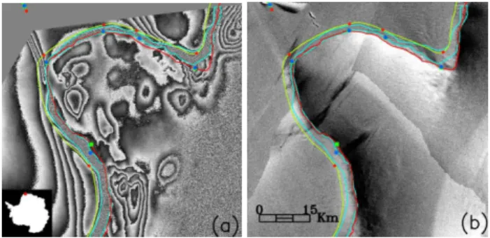
Figure 2 illustrates boundaries in the grounding zone from these different approaches for a portion of Antarctic margin near the Ekstr¨om Ice Shelf and Neumayer Station. There is broad agreement between the region of flexure zone, de-fined by the band of dense InSAR fringes, the Ib and H
points, defined by the GLAS analysis, and the delineation of the grounded ice boundary, interpreted from the Landsat imagery (discussed in more detail later). However there are some differences, such as in the upper left of the scene where the flexure zone narrows while the hydrostatic line, guided only by the few GLAS points, remains farther offshore. In the inlet near the upper right corner of Fig. 2, the ASAID
‐
Fig. 2. Section of Antarctic coast (Halvfarryggen Ridge on the Princess Martha Coast with Ekstr¨om Ice Shelf on left) 71.6 km×69.7 km comparing mappings of different features of the grounding zone with different methods. (a)Interferometric fringe pattern produced by InSAR methods and(b)an enhanced subset of the Landsat Image Mosaic of Antarctica. Cyan lines represent edges of the tidally flexed grounding zone between points F and H (see Fig. 1). Symbols are key points of the grounding zone iden-tified from repeat-track GLAS elevation profiles (F, green square; Ib, blue circle; H, red diamond). Red and green lines are ASAID
grounded ice boundary and hydrostatic lines, respectively.
grounded ice boundary passes farther inland than the band of dense InSAR fringes, but agrees with the Ib point (blue
circle) determined from GLAS data. There will always be some differences between boundaries within the grounding zone produced by these different methods, at times due to in-correct interpretation or data quality and availability, but also because different features are being detected. Our observa-tions of the differences between the different boundaries in the grounding zone determined by these various methods, now including the ASAID grounded ice boundary and hy-drostatic line, match those discussed and illustrated at greater length in Fricker et al. (2009).
Previous mappings of the “grounding line” based on satel-lite optical imagery have been produced and are available through data centers. Two of these familiar to many Antarc-tic researchers are the “grounding line” contained in the Antarctic Digital Database (ADD) (http://www.add.scar.org: 8080/add/index.jsp), where the latest revisions were based on prints of Landsat imagery at 1:250 000 scale, and a “ground-ing line” mapped from the MODIS Mosaic of Antarctica (MOA) at 125-m resolution (Bohlander and Scambos, 2007). A third partial mapping is being released incrementally as coastal change maps (Ferrigno et al., 1996 and http://pubs. usgs.gov/imap/2600/). Each of these mapped boundaries corresponds to either the most rapid change in surface slope (e.g., Ib in Fig. 1) or an end of grounded ice (in the case
‐
‐
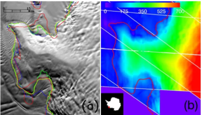
Fig. 3. Section of Antarctic coast (Scott Peninsula along Bakutis Coast) approximately 60 km×69 km. (a)Enhanced Landsat im-age comparing various imim-age-based mappings of the “grounding line” or grounded ice boundary: red, Antarctic Digital Database; blue, USGS Coastal Change map series; green, MODIS Mosaic of Antarctica; yellow, ASAID.(b)Color-coded surface elevations (in meters above mean sea level) derived from ASAID application of photoclinometry using image on left and GLAS elevation profiles. Thin white lines show the location of GLAS profiles interpolated by photoclinometry. ASAID grounded ice boundary from(a)is repro-duced (now in red).
some significant geolocation errors and it is possible some aerial photography may have been included since some por-tions of this persistently cloudy coast were never adequately imaged with the early Landsat instruments. Reduced spatial or feature acuity might have also contributed to the discrep-ancies in the ADD boundary. The MOA line is more accurate than the ADD in defining the overall shape of the coastal fea-ture, but at times deviates from the other interpretations when coastal features associated with lightly grounded ice and transitions to the floating ice shelf are encountered. There also are some differences between the USGS coastal change maps and ASAID that we attribute to the fact that the USGS procedure used paper prints of lower resolution Landsat im-ages while ASAID could vary the enhancement of any image in a digital environment to optimize the visual appearance of any local region as different conditions of topography and illumination orientation were encountered along the coast.
3 Data
The primary data sets used to define and provide surface ele-vations of the grounded ice boundary and hydrostatic line are images from the Enhanced Thematic Mapper Plus (ETM+) instrument onboard the Landsat-7 satellite and surface ele-vation profiles measured by the Geoscience Laser Altimeter System (GLAS) onboard the Ice, Cloud, and Land Elevation Satellite (ICESat). The Landsat data were used in the con-struction of the Landsat Image Mosaic of Antarctica, another IPY project (Bindschadler et al., 2008). This image set
con-sists of mostly cloud-free images. They also cluster within a relatively narrow time window (1999–2003). All images were accessed from the USGS EROS Data Center, usually by ftp-download after a visual review of possible candidate im-ages that cover the appropriate region of the ice sheet perime-ter. 196 images of this collection cover the entire grounded ice boundary to 82.5◦S. Farther south, two ASTER images provide coverage that complete the Ronne Ice Shelf por-tion of the grounded ice boundary, and imagery from MOA is used to complete the southernmost section of the Ross Ice Shelf. For all but the MOA imagery, the panchromatic band image was visually interpreted at full 15-m resolution (panchromatic band) to identify the grounded ice boundary (cf., Fig. 3a).
GLAS/ICESat data of precise surface elevation informa-tion along satellite groundtracks is used in three different ways. The first two uses employ the set of F, Iband H points
available from the National Snow and Ice Data Center (Brunt et al., 2010a). The locations of most rapid slope change Ib,
determined along single profiles are used to help confirm the identification of the grounded ice boundary based primarily on the imagery. The H locations, determined by a differ-encing technique employing repeat GLAS passes collected at different phases of the tide to reveal the tidal flexure of the ice shelf as described in Fricker et al. (2006), are used to determine the position of the hydrostatic line. The third use of the GLAS elevation profile data are in combination with the ETM+ images to produce surface elevation fields through application of photoclinometry (Wildey, 1975; Bindschadler and Vornberger, 1994).
4 Methods
To satisfy the IPY objectives of international collaboration and inspiring young researchers, the ASAID project invited partners across the world to participate. Customized software was created, along with appropriate documentation describ-ing standardized procedures so that the eventual aggregate product is as uniform as possible. The Antarctic perimeter was divided into a number of segments with different ASAID participants accepting responsibility for mapping portions of the grounded ice boundary and producing photoclinometric elevation fields for that segment (the hydrostatic line and el-evation selection were completed at the end of the project exclusively at NASA Goddard Space Flight Center). The software is designed so that the participant’s results are writ-ten to files with standardized names, facilitating both review of the data at NASA Goddard, but also easing the combi-nation of multiple participant results into a single aggregate. Ultimately, all data products were reviewed by the Principal Investigator (Bindschadler, 2010) and final responsibility for their content and quality rests there.
4.1 Grounded ice boundary
Our procedure starts with selecting a particular ETM+ image covering the desired section of the Antarctic perimeter and downloading it from USGS EROS Data Center website. The ASAID software uses the image metadata supplied with the image to determine the sun azimuth for the image and ro-tates the image to a sun-at-the-top orientation (required for the later photoclinometry procedures). The software then displays the rotated image on a computer monitor and su-perimposes the location of ICESat reference groundtracks on the image. Actual groundtracks usually lie within 100 m of the reference groundtracks. Next, to reduce computer mem-ory requirements and file sizes, the user defines sub-images to work on that encompass sections of the expected grounded ice boundary and include ICESat tracks near the top and bot-tom edges of the sub-image (so a photoclinometric elevation field spanning most of the sub-image can be produced). Once the sub-images are defined, each is written to a separate file directory and the GLAS data for that region are parsed from the complete set of GLAS data (provided to each ASAID user) and also written to the same directory. The GLAS data used are the GLA06 product (Release 28 and 29) from ob-servation periods 2A (4 October 2003 to 19 November 2003) through 3K (4 to 19 October 2008) (Zwally et al., 2003). Both releases include an ocean tide correction which was retained; however, the saturation correction (i satElevCorr) was only applied to Release 28 data as advised by ICE-Sat data product experts (J. Saba, personal communication, 2009). The processed files provide surface elevation values at ground points spaced roughly 172 m apart along the actual groundtracks.
At this point, the user visually reviews the individual GLAS profiles for each reference track (using customized ASAID software) and selects the profiles most suitable for photoclinometry. Only one profile for each reference track is permissible. Averaged profiles are not used because in-dividual profiles are often separated by tens and sometimes hundreds of meters and the individual laser footprint loca-tions are not aligned. The coastal region of Antarctica is of-ten cloudy, producing large and/or multiple gaps in the pro-files. Our application of photoclinometry requires a GLAS elevation both up-sun and down-sun as starting and ending points for the interpolated. In general, the “best” profiles se-lected are usually the most continuous profiles because they provide the most complete photoclinometrically derived ele-vations along the grounding ice boundary.
Photoclinometry is then applied within the sub-image to produce elevation values at all image points between GLAS profiles using interpolations based on the image pixel bright-nesses (Wildey, 1975; Bindschadler and Vornberger, 1994). The technique has been extensively developed for ice sheets where the existence of a homogenous surface of nearly con-stant albedo satisfies an important assumption for successful
application of the technique. Image pixel brightness is re-lated to surface slope by
DN=Acosθ+B (1)
where DN is the pixel brightness (in sensor units of digital number);θ is the angle between the solar illumination and the surface normal; coefficientAis the product of the solar irradiance, the surface reflectivity and the factor converting radiance to sensor DN units; andB is a bias due the sen-sor zero-radiance offset and atmospheric scattering (Bind-schadler and Vornberger, 1994). In most ice sheet situations,
Bis negligible and we also choose to make this assumption. Equation (1) is applied independently for each image seg-ment lying between an up-sun GLAS profile and a down-sun GLAS profile. Interpolation distances are kept as short as possible to minimize interpolation errors. To ensure that the GLAS profiles are continuous at the pixel scale, each pro-file is linearly interpolated across the standard GLAS point spacing of about 170 m as well across data gaps as large as 450 m. Larger gaps remain unfilled which can lead to longer interpolation segments and can create gaps in the el-evation field. For each image segment, Eq. (1) is applied after solving for that segment’s unique value of the scaling coefficient,A, using values of the average slope and image average brightness along that segment. This method ensures that the GLAS elevations along profiles remain unchanged although it can produce slight discontinuities between adja-cent image segments when the scaling parameter for adjaadja-cent image segments varies significantly. These cross-profile dis-continuities are sometimes referred to as “curtains” and are more severe the longer the interpolation segments become. The 8-bit quantization of Landsat DN values also contributes randomly to discontinuities between tracks. Alternative im-plementations of Eq. (1) were considered, but the GLAS data were deemed to be the best-known elevation information, so these values remain fixed. No attempt was made to smooth the resulting discontinuities because, in general, the calcu-lated elevation fields in constant albedo areas lacked artifacts such as these curtains. Figure 3b shows the photoclinometri-cally derived elevation field for the image in Fig. 3a as well as the pattern of selected GLAS profiles used as control for that elevation field. The angled boundaries of the elevation field in the lower portion of the figure result from the require-ment that there be an up-sun and down-sun GLAS elevation point for every interpolation segment.
of GLAS profiles, but also on the topographic variation of the region. Other, more sophisticated interpolation methods were examined, but they had the propensity for very large errors over sparsely sampled, undulated topography. Ulti-mately, our more conservative approach was deemed prefer-able because it provided an elevation value close to the GLAS values and is reliable in providing a value when no other elevation methods work.
At this stage, with the image providing a nadir view of the sub-image region and the derived elevation field provid-ing a view of the three-dimensional shape of the area, the boundary of the grounded ice features is drawn. Both data sets are linked in separate displayed windows on the com-puter monitor so that cursor movements can be followed in both windows. To assist the user, the displayed range of ei-ther gray-scale (of the image) or color scale (of the elevation field) can be adjusted and the user can zoom the displays to view detail at the 15-m pixel level. Guiding the cursor, the user either draws a continuous line, or clicks discrete points that the computer connects with linear segments, displaying the new grounded ice boundary on the image. The MOA “grounding line” is also displayed and provides useful guid-ance in areas where the ETM+ radiometric resolution (even with adjustable contrast applied by the user) fails to resolve important subtleties of the surface. In other areas, the in-creased spatial resolution of ETM+ enables corrections to the MODIS “grounding line” (cf., Fig. 3a).
The primary visual guide to tracing the precise location of the grounded ice boundary over most of the ice sheet perime-ter is the visual detection of a change in image brightness that corresponds to the localized slope break between a rela-tively steep slope on the grounded ice and a relarela-tively shallow slope seaward. The smoother surface of either the floating ice shelf or the fast sea ice relative to the more undulated sur-face associated with grounded ice features emphasizes this boundary. Marine features, such as offshore icebergs, sea ice lead and floe structures, or open ocean assist in identifying non-grounded regions. However, even with these numerous clues, defining the boundary at the full 15-m resolution is of-ten challenging because the spatial scale of the transition can be many pixels wide. In such regions, the ability to change the image enhancement and zoom to any scale greatly assists precise positioning of the grounded ice boundary. In some regions, the GLAS profiles are useful in precisely locating the point of maximum slope change and the software allows single profiles to be displayed with a linked cursor function that ties position along the profile to the image at the single pixel level.
Bare rock is very easily identified, but uncertainty garding the possible presence of seasonal snow often re-quires judgments as to the inclusion or exclusion of indi-vidual patches of bare rock within the ice sheet boundary. These situations often have a fractal nature to them and some smoothing is applied by both the operator’s initial drawing and by post-drawing software (described later) to be
practi-cal. Some false extension of the ice sheet is possible due to seasonal snow and future monitoring of the ice sheet bound-ary in regions prone to this effect should be evaluated care-fully.
The most challenging sections of the grounded ice bound-ary to identify are where fast-moving glaciers discharge into ice shelves. In these cases, the glacier is readily identified by surface undulations and the ice shelf by the absence of similar undulations, but the precise position of the boundary between the two is frequently difficult to locate accurately where the undulations become less dense and less distinct gradually. In general, the grounded ice boundary is drawn immediately seaward of the most downstream undulations and other features that appear to be formed by ice flow over regions of basal resistance and upstream of ice shelf features such as ice rumples or isolated ice rises. In these regions, the 8-bit radiometric resolution of the Landsat imagery often is stretched to its limit and the better 12-bit radiometric resolu-tion of the MODIS sensor enables detecresolu-tion of more subtle surface undulations. For this reason, in many outlet glacier cases, the MOA imagery is examined alongside the Land-sat imagery and, when the MOA imagery shows additional grounded ice features, the ASAID grounded ice boundary follows the trace of the MOA “grounding line”.
The typically shallow surface and bed slopes in this type of region are well documented and have led to the recognition of lightly grounded ice plains (Thomas et al., 1988; Alley et al., 1989; Corr et al., 2001). These areas also probably exhibit a wide grounding zone, so large differences between the grounded ice boundary, as we define the seaward limit of grounded ice features in the surface morphology, and the hinge line, as identified in InSAR or altimetry data, are to be expected. Nevertheless, the regions that contain visible sur-face expressions of grounded ice are regions where the ice feels the bed strongly enough that the shape of the ice ad-justs to the basal stresses, whereas the absence of these fea-tures indicates the ice does not feel the bed enough to change its shape and, with it, its internal stresses. This makes the grounded ice boundary a metric of the internal ice dynamics and, thus, is an important feature to map and to monitor, even on large fast outlet glaciers, regardless of its relation to the hinge line.
The work described above was completed for each sub-image, each in its own file directory. Combining these individual segments into a single continuous grounded ice boundary around the main ice sheet involves many addi-tional steps. Each sub-image’s grounded ice boundary is vi-sually reviewed and, if necessary, revised, amended or cor-rected. There were 319 individual boundary segments that were combined. Gaps and overlaps between segments are corrected with additional editing. The two largest gaps occur south of 82.5◦S, beyond Landsat coverage. On the Ronne Ice Shelf, three ASTER images are used in an equivalent manner and on the Ross Ice Shelf the MOA image is used, also as a proxy for Landsat imagery. In these areas, ICESat coverage
Fig. 4.The ASAID grounded ice boundary displayed on the Land-sat Image Mosaic of Antarctica. Line color represents the type of transition for ice transiting the grounded ice boundary. The cor-responding percent frequencies of occurrence are: Ice Shelf (dark blue, 61 %); Outlet Glacier (cyan, 13 %); Fast Ice (green, 10 %); Open Ocean (orange, 9 %); and Rock (red, 7 %).
is plentiful, and the photoclinometric elevation fields are high quality, providing an excellent information base from which the grounded ice boundary is drawn. Finally, to remove the unavoidable “jitters” and “stair-steps”, inherent in either a hand-drawn or piecewise-linear line, the drawn lines are smoothed before joining segments. The smoothing approach used a forward-looking algorithm wherein the direction of the redrawn grounded ice boundary is guided by the direc-tion of the next few drawn points rather than only the next point. The details of this approach are provided in separate documentation that will accompany the archived data files (discussed later).
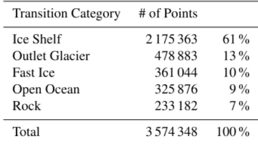
Figure 4 shows the final grounded ice boundary produced by these procedures. It is 53 610 km long and contains 3 574 365 points at a 15-m resolution. The convoluted na-ture is less apparent at this scale, but for comparison’s sake, the length of the 72◦ latitude line is 12 350 km. The col-ors in Fig. 4 indicate the nature of the ice transition at each point along the grounded ice boundary. Each boundary point was determined to be one of five categories: ice shelf; out-let glacier; fast (sea) ice; open ocean; and rock (or land). The number of points and percentage frequencies in each of these transition categories is given in Table 1. The common characteristics defining the outlet glacier class are: a spatially confined flow region, the presence of flow stripes oriented along the expected flow direction, and/or the presence of fea-tures on the ice shelf suggestive of a concentrated discharge from the grounded ice sheet. The extent of the outlet glacier was usually taken as the cross-flow “gate” and did not
in-Table 1.Distribution of Antarctic Ice Sheet Grounded Ice Bound-ary Categories.
Transition Category # of Points
Ice Shelf 2 175 363 61 %
Outlet Glacier 478 883 13 %
Fast Ice 361 044 10 %
Open Ocean 325 876 9 %
Rock 233 182 7 %
Total 3 574 348 100 %
clude any margin-parallel segment (that being assigned as an “ice shelf” transition). Differences between the categories of fast ice (which includes possible seasonal sea ice) and open ocean are ephemeral, depending on the specific date of the image used. On-land terminations, where the ice sheet thins to a vanishingly thin wedge adjacent to bare rock, are often highly convoluted and sometimes complicated by seasonal snow cover.
Nearly three-quarters (74 %) of the ice passing the grounded ice boundary transitions to an ice shelf (the com-bination of the ice shelf and outlet glacier categories). The fast ice and open ocean categories combine to a sub-total of 19 % of the grounded ice boundary, indicating that portion of the ice sheet that flows directly into the ocean and is not con-nected to an ice shelf fed by the grounded ice sheet. Finally, 7 % of the grounded ice boundary, the vast majority of which occurs in the Dry Valleys region near the northwest corner of the Ross Ice Shelf and the northeastern Antarctic Penin-sula, terminates on land above sea level. This relatively high value is associated with the extreme serpentine nature of the grounded ice boundary in these valley incised mountains and includes a few, relatively small, outlet glaciers that terminate on land.
4.2 Hydrostatic line
The hydrostatic line is mapped using the same ASAID soft-ware as the grounded ice boundary mapping, but rather than following a brightness feature in satellite imagery, it is drawn such that it is tied to each H point supplied in the F/Ib/H
data set derived from repeat-track analysis of GLAS profiles (Brunt et al., 2010a). Between these points, the hydrostatic line is drawn to reflect the general shape of the grounded ice boundary. The smoother shape of the hydrostatic line is intentional, expressing the diffusion of beam supporting stresses onto the ice shelf as has been noticed in interfero-metric data analyses.
shelf or to an outlet glacier, but includes a few places where the grounded ice boundary wraps around a coastal nunatak and a continuous ice shelf exists on the seaward side of that nunatak. In some areas, there are no, or widely spaced H points, however, in general, the seaward offset of the hydro-static line from the grounded ice boundary varies only slowly along the hydrostatic line, increasing our confidence that a reasonably accurate mapping of this feature is possible. An analysis of the seaward offset of the hydrostatic line from the grounded ice boundary appears later. Overall the hydrostatic line contains approximately 1.67×10⁶points for a total dis-tance of 27 521 km, considerably shorter than the grounded ice boundary, reflecting its smoother, discontinuous nature.
While some segments of the ASAID hydrostatic line are poorly constrained by wide spacings between the H points, there are at least two reasons to attempt its definition. The first is associated with the ultimate goal of ASAID which is to quantify ice discharge. The H point is defined as the point on an ice shelf closest to land that responds fully to tidal oscillations (Fricker and Padman, 2006). Thus its free-board is independent of the tidal amplitude and its thickness can be calculated from its surface elevation if the densities of the ice shelf and sea water are known. This enables a means to calculate ice thickness and, when combined with surface velocity (equal to column-averaged velocity on an ice shelf), the discharge can be calculated. This is a valu-able set of conditions and even though such discharge cal-culations will not include basal melting landward of the hy-drostatic line, when combined with discharge values at either the hinge line or the grounded ice boundary, they represent another discharge gate and will contribute to quantifying the basal melt between the more-landward gate and the hydro-static line. A second, more general, reason to map the hy-drostatic line is that, just as the grounded ice boundary repre-sents a dynamic boundary separating ice that feels (and does not feel) the bed stresses sufficiently to affect the geometry of the ice, the hydrostatic line represents the boundary be-yond which the beam stresses transmitted by the grounded ice sheet through the most-landward portion of the ice shelf are no longer felt. Thus, the hydrostatic line represents an-other type of dynamic boundary directly related to the trans-mission of stresses through the ice. As conditions within and around the ice shelf change, the position of the hydrostatic line will change, so mapping and monitoring the hydrostatic line holds the promise of identifying change at the sensi-tive margins of the Antarctic ice sheet and can be a check on changes inferred from changes in the position of other marginal boundaries (e.g., the hinge line or the grounded ice boundary).
4.3 Positional accuracy
Landsat-7 imagery has a general geo-registration precision of 50 m (one-sigma) (Lee et al., 2004). This precision was con-firmed by the misfits experienced with the imagery when the
Landsat Image Mosaic of Antarctica (LIMA) was produced (Bindschadler et al., 2008). Each image was orthorectified, using the RADARSAT Version-2 DEM as part of the LIMA image processing procedure, so this correction is included in the Landsat images used here. Later we establish that in the coastal areas the RADARSAT Version-2 DEM contains er-rors, as do other DEMs, and while these are generally a few tens of meters, they can exceed 100 m in places. Viewing angles in Landsat imagery are small (less than 10◦at the im-age edge) limiting the impact of orthorectification errors on positional errors, and the elevations along the grounded ice boundary are only a few tens of meters. The end result is that orthorectification-induced positional errors are less than 15 % of the elevation error and can be neglected in most cases.
The error in the identification of the grounded ice bound-ary on an image varies with the nature of the boundbound-ary. When the transition type is either open ocean or rock, the boundary is able to be drawn to the nearest pixel. When a sea-ice transi-tion occurs, the boundary is slightly less obvious, depending on the height difference between the surfaces of the grounded ice and the sea ice and the orientation of the sun relative to the direction of the transition boundary. In general, this bound-ary can be determined to two pixels (30 m). When the tran-sition consists of slowly flowing grounded ice flowing into a floating ice shelf, the slope break is usually prominent and by zooming in sufficiently to resolve individual pixels, the boundary can be traced to the nearest 3 pixels (45 m). The grounded ice boundary is extremely serpentine. This charac-ter limits instances where a slope break is hard to see because it is both straight and oriented in the direction of the solar il-lumination. The least accurate delineation of the grounded ice boundary is across the mouths of outlet glaciers and ice streams. Here the accuracy varies enormously, based primar-ily on the spatial density and magnitude of the grounded ice features. As discussed above, the MODIS-based “ground-ing line” is often relied upon in these instances, but even in that lower resolution image space, the grounded ice features have diffuse edges so we assign a four MODIS pixel error (500 m) error to this boundary. The georegistration and de-lineation errors are the two major sources of positional error, so overall, our estimates of the positional errors (one-sigma) for the grounded ice boundary are the root-squared-sum of these two contributions:±52 m for the open ocean and rock boundaries;±58 m for the sea ice boundaries;±67 m for the ice shelf boundaries; and a much larger±502 m for the outlet glacier boundaries.
The positional accuracy of the hydrostatic line is much poorer. This line is pinned to the H points determined from the repeat ICESat pass analysis and interpolated in be-tween. The positional uncertainty of individual H points from all factors included in their estimation method is stated as ∼2000 m (Brunt et al., 2010b). Interpolation of the hy-drostatic line is only guided by the shape of the nearby grounded ice boundary and likely introduces a few additional
kilometers error. As such, we view the ASAID hydrostatic line as an initial estimate of the actual position that will be significantly revised once additional repeat pass altimetry or InSAR data of sufficient precision are collected and ana-lyzed.
4.4 Elevations
In the coastal regions of Antarctica, the assumptions required for accurate photoclinometry are violated frequently enough and GLAS elevations are sparse enough that the assignment of elevations to points along either the grounded ice bound-ary or the hydrostatic line requires the consideration of addi-tional digital elevation models (DEMs). There are a number to choose from, but each has weaknesses in particular regions or is incomplete, so no single elevation data set is sufficient by itself. Thus, our approach considers a number of elevation values in parallel and allows us to select the “best” elevation values based on their adherence to both nearby GLAS data and the shape of the local ice sheet surface inferred from the Landsat imagery and the GLAS data.
The elevation data sets considered include the photoclino-metric and triangulation DEMs already discussed. In addi-tion, a DEM based on a combination of radar and laser satel-lite altimetry (Bamber et al., 2009) and another based primar-ily on elevations in the Antarctic Digital Database (ADD) in coastal areas and ERS-1 radar altimetry in the ice sheet in-terior which was used by the RADARSAT project data (Liu et al., 2001) are included. The former, called here the “al-timetry” DEM, specifies surface elevations on 1-km postings while the RADARSAT Version-2 DEM provides elevations on 400-m postings. Both are resampled to our 15 m grid using a bi-linear interpolation scheme. Finally, two stereo image-based photogrammetric DEMs are included: the G-DEM based on ASTER stereo imagery (http://www.ersdac. or.jp/GDEM/E/index.html) and, in a few available areas, lo-cal DEMs based on stereo SPOT imagery provided by the SPIRIT project (another IPY activity) (Korona et al., 2009). All elevation data sets are converted to a common mean sea level reference by using the EGM96 geoid referenced to the WGS-84 ellipsoid.
Additional customized software was developed to accom-modate the needs of this elevation-selection task. The work returns to the sub-image level because the photoclinometric and triangulation DEMs exist only for each separate sub-image. For any sub-image, each DEM grid is interpolated to extract that DEM’s elevation values along the trace of the grounded ice boundary. These boundary-following elevation profiles are superimposed on a single display plot (using dis-tinct colors for each DEM) along with single elevation val-ues corresponding to where GLAS elevation profiles cross the grounded ice boundary. Figure 5 shows an example of the computer screen produced by this software. In addi-tional on-screen windows, the photoclinometric, altimetric, RADARSAT and ASTER DEMs are displayed as shaded
re-lief images, rotated and illuminated to simulate the original Landsat sub-image. These shaded relief images are an ex-cellent means to highlight subtle artifacts in each DEM, pro-viding another test of each DEM’s fidelity in matching the surface topography (cf., Fig. 5).
With this visual information, the operator is able to se-lect a portion of the grounded ice boundary, define the best source of elevation data along that segment, and assign a quality (or confidence) rating to those elevations. GLAS data are regarded as “truth”, so elevation values close to the GLAS data are weighted heavily in choosing the preferred elevation source, as well as in rating its quality, but a pro-file that matches the perceived shape of the surface along the grounded ice boundary is also important. The ability to de-fine the preferred elevation in segments based on the relative, and shifting, strengths of the various elevation sources re-moves the dependence of the chosen elevations on a single elevation source and is both a critical software feature and an important characteristic of the ASAID products. Further, the ability to define the beginning and ending of each seg-ment enables the preferred DEM source to switch at crossing points, thus avoiding a discontinuity in the profile of chosen elevations. Not all discontinuities are avoided, however, par-ticularly in the case of small gaps in an otherwise preferred DEM. This was especially true for the SPIRIT DEMs that cover only limited areas and for the ASTER G-DEM that is hampered by the application of an inaccurate coastal mask that omits elevations in regions where it appears that excel-lent elevations might have been provided in the unmasked, but unfortunately unavailable, DEM. Where discontinuities occur, the quality rating is set to “Poor” (least confident rat-ing) to acknowledge the fact that at least one chosen elevation is incorrect. An additional selectable elevation of “sea level” is available to identify the many instances of the grounded ice boundary occurring with a transition to the open ocean. No DEM correctly captures the elevation discontinuity at these locations. In these cases, the DEMs are ignored and an eleva-tion of zero is specified. This occurs in 9 % of the grounded ice boundary points (cf., Fig. 4 and Table 1).
‐
‐
‐
Fig. 5.Sample of screen display for elevation selection operation.(a–c)Shaded relief versions of photoclinometric, altimetric (aka. Bamber, 2009) and Radarsat DEMs, respectively, rotated and illuminated to match the original illumination of the Landsat sub-image. Blue line is the ASAID grounded ice boundary; green line is the MOA “grounding line”. Red “+” symbols correspond to position of vertical dashed red line in lower panel.(d)Elevation profiles extracted from various DEMs indicated by lines of different color (legend below) with red X’s being ICESat GLAS elevation values positioned where the ICESat profiles crosses the grounded ice boundary. Horizontal axis is in units of 15-m pixels. Vertical axis is elevation in meters above sea level.
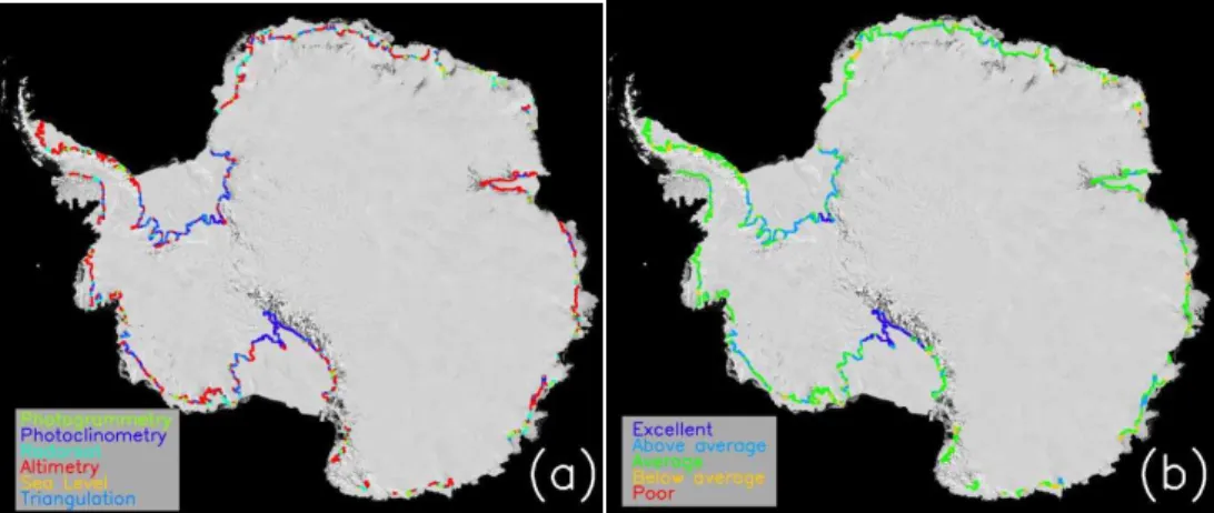
Figure 6. The ASAID grounded ice boundary. (a) Colored lines represent the DEM source of selected
Fig. 6. The ASAID grounded ice boundary. (a)Colored lines represent the DEM source of selected elevation values. The corresponding percent frequencies of occurrence are: photogrammetry (green, 33 %); photoclinometry (dark blue, 26 %); Radarsat (cyan, 17 %); altimetry (red, 13 %); sea level (orange, 9 %); and triangulation (light blue, 2 %).(b)Colored lines represent the confidence in the selected elevations. The corresponding percent frequencies of occurrence are: Excellent (dark blue, 18 %); Above Average (cyan, 36 %); Average (green, 40 %); Below Average (orange, 5 %); and Poor (red, 0.5 %).
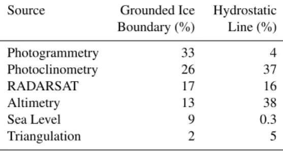
Table 2.Elevation Source for points along grounded ice boundary and hydrostatic line.
Source Grounded Ice Hydrostatic Boundary (%) Line (%)
Photogrammetry 33 4
Photoclinometry 26 37
RADARSAT 17 16
Altimetry 13 38
Sea Level 9 0.3
Triangulation 2 5
the time, the next most used elevation source, with the largest region of use being along the grounded ice boundary of the Ronne/Filchner Ice Shelf. RADARSAT and the altimetric DEMs were used 17 % and 13 % of the time, respectively. The triangulation elevations, a worst-case alternative, only needed to be used 2 % of the time.
Table 3 summarizes the frequency of the selected eleva-tions for each confidence class and Fig. 6b shows the spa-tial distribution. Quantitative accuracies are discussed in the next section. The “Excellent” ranking, reserved for those segments where the elevations matched the GLAS eleva-tions very closely, occurs 18 % of the time and is largely confined to the southernmost boundaries of the Ross and Ronne/Filchner Ice Shelves. “Above Average” confidence (36 % occurrence) is assigned to segments along which there is close agreement with the GLAS elevations and the shape of the profile agrees with a visual interpretation of the im-agery (i.e., the simulated image and the actual image were similar). This category also is located most frequently at ice shelf transitions, but is more widespread throughout West Antarctica. Segments ranked with an “Average” confidence in elevations (40 % occurrence) display more variations be-tween DEMs but with a clear preference for the one DEM and are distributed along the entire boundary. “Below Av-erage” confidence (5 % occurrence) usually corresponds to cases where the spread of DEMs is large with none standing out as the obvious choice. In these cases, the preference was usually assigned to the DEM profile that either most closely matches the GLAS elevations or that best expresses the shape of the elevation surface interpreted from the imagery. These are seen to occur in very isolated regions. In the cases of “Poor” confidence (0.5 % occurrence), there were no good elevations to choose from or there are elevation discontinu-ities along the boundary.
To ensure consistent application of this qualitative confi-dence assessment throughout the entire data set, the ratings were assigned by a single operator. The spatial pattern of confidence is not obviously correlated with the specific type of boundary – from rugged mountains to very smooth, nearly featureless terrain, to heavily crevassed regions – so its
inclu-Table 3.Elevation Confidence for points along grounded ice bound-ary and hydrostatic line.
Grounded Ice Hydrostatic Boundary (%) Line (%)
Excellent 18 4
Above Average 36 32
Average 40 59
Below Average 5 4
Poor 0.5 0.1
sion in the ASAID product provides an additional indication of elevation accuracy that cannot be gleaned from knowing either the type of transition or the source DEM.
The identical elevation-picking procedure is applied to the hydrostatic line. Figure 7 and Tables 2 and 3 present simi-lar results for the hydrostatic line. The selections and statis-tics of the preferred elevation sources are distinctly different from those for the grounded ice boundary. In particular, pho-togrammetry is only selected 4 % of the time and is limited to the rougher coasts. This decrease in use is due to three factors: photogrammetry is most accurate in rugged terrain, where there are sharp features in the stereo imagery, but ice shelves tend to lack these features; there often is no hydro-static line (i.e., no ice shelf) near some of these areas; and when there is a hydrostatic line, the frequently poor mask-ing of the ASTER G-DEM eliminated potentially useful el-evations in these regions. In its stead, at 38 % of the total, altimetry makes a much larger contribution to the chosen hy-drostatic line elevations and is distributed across the coast. This is probably due to the smoothing effect of fitting an el-evation surface to the altimetric data: a bias toward higher elevations will result at the grounded ice boundary where the slope change is most rapid, but this bias will be much reduced farther out on the ice shelf. Photoclinometry also increases its share of the selected elevations, to 37 %, because it works best in less rugged terrain and uncrevassed regions, but its distribution is still strongly confined to the same regions as for the grounded ice boundary. RADARSAT elevations are used about as frequently for the hydrostatic line (16 %) as for the grounded ice boundary (17 %) but with no particu-lar spatial concentration. Sea level (zero elevation) is chosen less frequently (0.3 %) because the hydrostatic line is not in-cluded in open ocean regions.
580 R. Bindschadler et al.: Getting around Antarctica
Figure 7. The ASAID hydrostatic line. (a) Colored lines represent the DEM source of selected elevation
Fig. 7. The ASAID hydrostatic line. (a)Colored lines represent the DEM source of selected elevation values. The corresponding percent frequencies of occurrence are: photogrammetry (green, 4 %); photoclinometry (dark blue, 37 %); Radarsat (cyan, 16 %); altimetry (red, 38 %); sea level (orange, 0.3 %); and triangulation (light blue, 5 %). (b)Colored lines represent the confidence in the selected elevations. The corresponding percent frequencies of occurrence are: Excellent (dark blue, 4 %); Above Average (cyan, 32 %); Average (green, 59 %); Below Average (orange, 4 %); and Poor (red, 0.1 %).
Average”. “Average” confidence is assigned to the major-ity (59 %) of hydrostatic line points, covering most of the coast. “Below Average” and “Poor” confidences are assigned to only 4 % and 0.1 % of points, respectively.
4.5 Elevation accuracy
Our elevation selection process includes many elevation sources and demonstrates that none are singularly preferred. To assess the accuracy of our chosen elevations, we com-pare them to two sets of field data. The first comes from an airborne mission conducted by the British Antarctic Survey (BAS) in the 2006–2007 austral summer, partly to support ASAID validation efforts. Surface elevations and ice thick-nesses were measured over approximately 1500 flight kilo-meters along extensive reaches of the western boundary of the Ronne Ice Shelf from 200 km north of Evans Ice Stream to the north margin of Institute Ice Stream. Because the ASAID mapping of this region had not been completed at the time these data were collected, they do not directly coincide with either the ASAID grounded ice boundary or the hydro-static line. However, because photoclinometry produces the preferred elevations in this region and this method produces an elevation field at 15-m spatial resolution, a direct com-parison of ASAID elevations near the grounded ice bound-ary and hydrostatic line with BAS measurements at identical locations is possible. The confidence for all the ASAID ele-vations in this area is divided roughly equally between “Ex-cellent” and “Above Average” (cf. Figs. 6b and 7b). 30 000 points spanning roughly 640 km are used covering the re-gions of Evans Ice Stream (and northward), across Carlson Inlet and around most of Fletcher Promontory. For each BAS measurement, its location is paired with the calculated eleva-tion of the nearest pixel in the photoclinometry DEM and
shown in Fig. 8. The linear fit through this distribution and forced to pass through (0, 0) has a slope of 0.997 and an
R2of 0.986. The elevation differences (BAS minus ASAID) produced a Gaussian distribution with a mean difference of 0.24±5.77 m. This region is experiencing a slight thicken-ing of about 0.2 m yr−1 (Pritchard et al., 2009). No large
elevation difference is expected because the 2006–2007 pe-riod of BAS data collection occurs roughly in the middle of the GLAS data time window (late 2003 to late 2008) and the GLAS data are used to control our photoclinometry eleva-tions.
The second comparison of elevations draws upon the BEDMAP compilation of Antarctic field data (Lythe et al., 2001). Although BEDMAP’s primary aim is to produce the best bed elevation map of Antarctica using all available mea-surements of ice thickness and surface elevation collected over the past 50 yr, some of the missions do include sur-face elevation data. The extended period represented by the data leave open the question of how much surface elevations may actually have changed from the time of collection to the epoch of our data sets. In addition, the elevation refer-ence surfaces (i.e., geoid and ellipsoid) also have evolved and some of the documents supporting particular BEDMAP mis-sions lack detail on this critical point. Despite these limita-tions, the BEDMAP data provide an independent and useful set of surface elevations to compare with the ASAID eleva-tions.
The vast majority of the 127 missions compiled by BEDMAP cover interior regions of the ice sheet, but a few contain data that cross the ASAID grounded ice bound-ary, the hydrostatic line, or both. Crossings are defined as any ASAID point (of either line) that occurs within 30 m of a BEDMAP data point. Other distances were tried, but a shorter distance missed some crossings while a larger
Fig. 8. Surface elevations measured by British Antarctic Survey near grounded ice boundary of Ronne Ice Shelf versus surface el-evations at the same locations extracted from a photoclinometry DEM produced by ASAID.
distance includes too many ASAID points for a single cross-ing. 15 missions yield 954 crossing point pairs of the grounded ice boundary and 702 crossing point pairs of the hydrostatic line, clustered on the three largest ice shelves: the Ross, the Ronne/Filchner, and the Amery. Very few ad-ditional crossings result from the other missions and because the statistics would not be altered significantly even if they were included, we limit our comparisons presented here to the BEDMAP data in these three areas. These areas are not among the areas experiencing the greatest rates of thickness change (e.g., Pritchard et al., 2009) so the risk of temporal elevation changes compromising our results is reduced.
Because some BEDMAP data sets do not include surface elevations, the number of crossing point pairs for which ele-vations can be compared is less than the number of crossings. Figure 9 plots the BEDMAP surface elevations against the paired ASAID surface elevations (including an indication of the chosen DEM source) of the ASAID grounded ice bound-ary and Table 4 presents the statistics of both the grounded ice boundary and hydrostatic line comparisons. The data pairs in Fig. 9 are distributed roughly equally on either side of a line of slope 1. The statistical linear fits, forced to inter-sect the origin (0, 0), considered separately for the 417 pairs of the grounded ice boundary subset and the 262 pairs of the hydrostatic line subset are nearly identical in slope (0.93 and 0.95, respectively) andR2(0.64 and 0.66, respectively). There appears to be no strong bias in these comparisons that is related to the selected DEM source with the exception that the Radarsat DEM seems to be biased slightly lower than the BEDMAP elevations.
Fig. 9. Surface elevations at common locations along the ASAID grounded ice boundary extracted from BEDMAP missions ver-sus preferred surface elevations selected from various DEMs by ASAID. Data symbols identify the source DEM used by ASAID. Sloped line is a linear fit through all points constrained to pass through (0, 0) (cf. Table 4).
Table 4.Comparison of BEDMAP and ASAID Surface Elevations. Slope andR2values refer to linear fits forced to pass through (0, 0) (cf., Fig. 9).
Number of Slope of R2 Elevation Difference paired points Linear Fit (m) (BEDMAP-ASAID)
Grounded Ice Boundary
All Classes 417 0.93 0.64 −4.7±26.4
Excellent only 58 0.75 0.81 −20.8±19.7
Above Average only 92 0.95 0.57 −3.6±28.9
Average only 261 0.94 0.66 −2.7±24.9
Hydrostatic Line
All Classes 262 0.95 0.66 1.5±21.5
Excellent only 0
Above Average only 89 0.91 0.67 5.4±23.0
Average only 163 0.98 0.65 −1.0±20.7
Below Average only 10 8.1±13.4
4.6 Ice thickness
Surface elevations on floating ice are sometimes converted to ice thicknesses by invoking the hydrostatic equilibrium con-dition. While this conversion is sometimes applied immedi-ately adjacent to the grounding ice sheet (e.g., Rignot et al., 2008), it is strictly only valid at the hydrostatic line, seaward of the hydrostatic line, and possibly at one or more locations between F and Im(see Rignot et al., 2011, Fig. 1 for this final
point). The conversion relationship can be written as
He=
(Zs−1h)ρw
ρw−ρi
; 1h=hf
1−ρf
ρi
(2) whereHe, is the equivalent ice thickness;Zs is the surface
elevation above mean sea level,hfandρfare the depth and
density of the firn, respectively; andρi andρware the
den-sities of pure ice and of seawater: 917 and 1026 kg m−3,
re-spectively. The term1his commonly referred to as the “firn-depth correction” and accounts for the air contained in the surface snow. A detailed meteorological model quantifying this air-in-firn effect has been published by van den Broeke et al. (2008). We were provided a file specifying the correction term on a 0.1 degree grid over the Antarctic continent that we bi-linearly interpolate to the location of each point along the grounded ice boundary and hydrostatic line. The distribution of this firn correction term around the perimeter of Antarctic was confirmed to be equivalent to Fig. 4 in van den Broeke et al. (2008).
In applying Eq. (2), there are a few instances where the firn-depth correction exceeds our surface elevation leading to negative equivalent ice thicknesses. This is clearly incorrect. Such occurrences are distributed widely around the continent and are often associated with where our hydrostatic line ex-tends across short patches of fast ice between longer sections
of floating ice shelf. The single largest concentration of very low elevations occurs between longitudes 40◦E and 57◦E. To avoid negative thicknesses, a variable coefficient is added to Eq. (2) modifying it to
He=
(Zs−f 1h)ρw
ρw−ρi
;f=1−e−Z1hs (3)
The coefficient,f, is only significant when the firn correc-tion depth becomes a significant fraccorrec-tion of the surface eleva-tion.f ranges from unity for large surface elevations to zero when the firn-depth correction is much larger than the sur-face elevation. Physically this coefficient can be interpreted as reducing the effect of included air in firn when the surface elevation is so low that much of that firn would be flooded by seawater and, presumably refrozen, thus increasing the density and reducing the air content.
Figure 10a shows the distribution of calculated hydrostatic line ice thicknesses around the continent along with a his-togram of values. Very thick ice (sometimes over 2000 m) occurs where deep ice streams and glaciers feed the Ross, Ronne/Filchner and Amery ice shelves. The histogram of ice thicknesses (Fig. 10b) approximates a log-normal distri-bution with the most frequent ice thicknesses in the range 300–400 m. There are two other features to note. The first is the local minimum/local maximum couplet at 800–900 m thickness. We offer no explanation for this feature nor do we associate any significant characteristic of hydrostatic line ice thickness to it. The second feature is the high frequency of occurrence at very small ice thicknesses; 6 % of the equiva-lent ice thicknesses are less than one meter. This might be a real feature, reflecting the frequent occurrence of thin ice, but it also is caused, to some undetermined degree, by errors in measurement of thin coastal ice and the accuracy of geoid knowledge along the Antarctic coast.
‐
Fig. 10. Ice thickness calculated along the ASAID hydrostatic line(a)mapped on the Landsat Image Mosaic of Antarctica with color representing ice-equivalent thickness in meters (cf., Eq. 3 in text) and(b)presented as a histogram of values.
4.7 Ice thickness accuracy
Our quantitative assessment of ice thickness accuracy uses the same BEDMAP data set employed earlier to assess el-evation accuracy. However, unlike those elel-evation compar-isons, ice thickness comparisons are not encumbered by the uncertainty of using a consistent reference surface. There also are more data pairs to compare, because all BEDMAP data sets include ice thickness. The same criterion of pairing each BEDMAP point to any ASAID point within 30 m is ap-plied and, repeating the results, there are 954 crossing point pairs of the grounded ice boundary and 702 crossing point pairs of the hydrostatic line, clustered on the three largest ice shelves: the Ross, the Ronne/Filchner, and the Amery.
To permit a valid comparison, the ASAID ice thicknesses are first converted from an ice-equivalent thickness to an ex-pected actual ice thickness by accounting for the firn-depth correction included in Eqs. (2) and (3). This is simply done by calculating the expected actual ice-shelf thickness,Haas
Ha=Zs+He
ρ
i
ρw
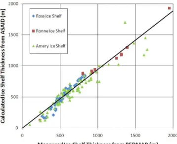
(4) Figure 11 plots the measured BEDMAP ice-shelf thickness values against the calculated ASAID values of actual ice-shelf thickness (Hafrom Eq. 4) for the crossing pairs along
the hydrostatic line and Table 5 presents the statistical results. The agreement is considerably better than for the surface el-evation comparison (cf. Fig. 9 and Table 4). The linear fit (again forced to intersect the origin (0, 0)) has a slope of 0.94 and anR2value of 0.92 with similar results when each of the three areas is considered separately: slopes ranging from 0.90 to 0.97 andR2ranging from 0.89 to 0.98 (cf., Ta-ble 5). The distributions of ice thickness differences indicate a consistent bias of ASAID calculated ice thickness lower than the BEDMAP-compiled ice thicknesses, although the magnitude of this bias, 41.2 m for all points, varies with the
‐
Fig. 11.Ice shelf thickness at common points along the ASAID hy-drostatic line extracted from BEDMAP mission measurements ver-sus actual ice thickness calculated from ASAID preferred surface elevations (as described in the text). Data symbols distinguish the three ice shelf regions. Sloped line is a linear fit through all points constrained to pass through (0, 0) (cf. Table 5).
area considered and it is less than one-sigma from zero. It is difficult to identify the source of these differences: real thick-ness change between the collection times of the data sets, location errors, errors in the ASAID elevation and firn-depth correction errors could all be factors. The Ross Ice Shelf area exhibits the best agreement: 23.6±44.2 m and is the data set collected with the least time difference between data sets.
Table 5.Comparison of BEDMAP and ASAID Actual Ice Thicknesses. Slope andR2values refer to linear fits forced to pass through (0, 0) (cf., Figs. 11 and 12). BEDMAP mission numbers refer to the specific source data sets.
Number of BEDMAP Slope of R2 Ice thickness Difference paired points Missions Linear Fit (m) (BEDMAP-ASAID)
Grounded Ice Boundary
All points 954 1.03 0.23 −57.3±12.1
Ross Ice Shelf only 508 42, 53 0.99 0.86 9.1±53.5
Ronne Ice Shelf only 25 34, 35, 37, 44, 74 0.95 0.91 86±120.9
Amery Ice Shelf only 417 7–9 and 68–73 1.09 0.05 −139±380
Hydrostatic Line
All points 702 0.94 0.92 41.2±71.3
Ross Ice Shelf only 231 42, 53 0.90 0.89 23.6±44.2
Ronne Ice Shelf only 26 35, 36, 37, 38, 44 0.96 0.98 56.8±62.9 Amery Ice Shelf only 445 5, 6, 9 and 69–74 0.97 0.92 73.5±98.1
Excellent only 341 1.19 0.98 14.3±29.6
Above Average only 162 0.91 0.93 68.7±79.9
Average only 190 0.91 0.91 66.6±94.7
decreases (cf., Table 5). These trends support our intention of providing users of these data sets a useful guide to indicate the variable accuracy of the elevations (and ice thicknesses derived from them). Applying Eqs. (2) and (4) to these ice thickness accuracies in Table 5, equivalent uncertainties in surface elevation can be extracted. The values are: ±3.6, ±9.6 and±11.4 for Excellent, Above Average and Average confidence levels, respectively. Without sufficient data pairs, the uncertainties for confidence levels 4 and 5 remain unde-termined by this procedure, but we estimate them to be±30 and±100 m based on the conditions used to assign them (i.e, the spread among various DEMs and the occasional occur-rence of discontinuities).
It has been stated repeatedly that hydrostatic equilibrium does not apply landward of the hydrostatic line. For this reason and to inhibit misuse of the grounded ice boundary data set, the ASAID data sets do not calculate an ice thick-ness from the preferred surface elevation along this bound-ary (although the firn-depth correction is provided for those who wish to take this risky step). However, to examine the magnitude of errors that would be made by assuming hydro-static equilibrium at the grounded ice boundary, here we con-vert our ASAID surface elevations to hydrostatically equili-brated ice thicknesses at the grounded ice boundary points close to BEDMAP points and compare them to BEDMAP values. The procedure to convert the surface elevations to actual ice thicknesses is identical to the procedure described above for the hydrostatic line points. The point pairs are plot-ted in Fig. 12 and statistics summarized in Table 5 but, in this case, the points are subdivided by region. Grounded ice is expected to have surface elevations higher than if it were floating in hydrostatic equilibrium, so a bias of
thicker-than-
Fig. 12.Actual measured ice thickness at common points along the ASAID grounded ice boundary extracted from BEDMAP mission data versus actual ice thickness calculated from ASAID preferred surface elevations. Data symbols distinguish the three ice shelf re-gions. Sloped line is a linear fit through all points constrained to pass through (0, 0) (cf. Table 5).
measured ice for the ASAID points is expected. Overall, this bias is apparent in Fig. 12, but when the comparisons are ex-amined separately for the three ice shelves, the agreement on the Ross Ice Shelf is comparable to that for the hydro-static line, the agreement on the Ronne Ice Shelf is somewhat equivocal and not well sampled, while it is the Amery Ice Shelf points that produce the expected too-thick ice bias. A possible explanation for the favorable agreement for the Ross