www.geosci-instrum-method-data-syst.net/4/81/2015/ doi:10.5194/gi-4-81-2015
© Author(s) 2015. CC Attribution 3.0 License.
High-frequency performance of electric field sensors aboard
the RESONANCE satellite
M. Sampl1,*, W. Macher1, C. Gruber1,**, T. Oswald1,***, M. Kapper1, H. O. Rucker1,****, and M. Mogilevsky2
1Space Research Institute, Austrian Academy of Sciences, Graz, Austria 2Space Research Institute, Russian Academy of Sciences, Moscow, Russia *now at: KATHREIN-Werke KG, Rosenheim, Germany
**now at: Karl Franzens University Graz, Institute of Physics, Graz, Austria ***now at: Thomas Oswald Aerospace Software, Weinitzen, Austria
****now at: Austrian Academy of Sciences, Commission for Astronomy, Graz, Austria
Correspondence to:M. Sampl (manfred.sampl@ieee.org)
Received: 1 August 2014 – Published in Geosci. Instrum. Method. Data Syst. Discuss.: 18 December 2014 Revised: 28 March 2015 – Accepted: 11 April 2015 – Published: 4 May 2015
Abstract. We present the high-frequency properties of the eight electric field sensors as proposed to be launched on the spacecraft “RESONANCE” in the near future. Due to the close proximity of the conducting spacecraft body, the sensors (antennas) have complex receiving features and need to be well understood for an optimal mission and spacecraft design. An optimal configuration and precise understanding of the sensor and antenna characteristics is also vital for the proper performance of spaceborne scientific instrumentation and the corresponding data analysis. The provided results are particularly interesting with regard to the planned mu-tual impedance experiment for measuring plasma parame-ters. Our computational results describe the extreme depen-dency of the sensor system with regard to wave incident di-rection and frequency, and provides the full description of the sensor system as a multi-port scatterer. In particular, go-niopolarimetry techniques like polarization analysis and di-rection finding depend crucially on the presented antenna characteristics.
1 The RESONANCE project
The RESONANCE project is dedicated to the investigation of properties and features of Earth’s auroral acceleration zone as well as near-equatorial phenomena. The missions over-arching goal is to study wave-particle interactions in the inner magnetosphere. Features to be observed include the
energy transfer between energetic particle species, particle precipitation, the magnetospheric cyclotron maser and the generation of planetary radio emissions (Demekhov et al., 2003) such as the auroral kilometric radiation. Comprised of four satellites and flying a magneto-synchronous formation, the mission seems ideal for the investigation of effects and processes which are occurring along the geomagnetic flux tubes. Of particular interest is the energy exchange between the ionospheric and magnetospheric layers of Earth’s atmo-sphere. Compared to previous radio science missions (cf. Ta-ble 1; Boudjada et al., 2010), RESONANCE provides the unique feature of sampling the same physical parameters in two space regions belonging to the same magnetic flux tube. The mission features, as well as the proposed spacecraft de-sign, have already been described in Mogilevsky et al. (2002, 2013).
Table 1.Overview of selected science missions and instruments
as-sociated with auroral radio emissions
Spacecraft Receiver Stokes
(Experiment) features components
0–10 Hz I, Q, U, V
RESONANCE 10 Hz–20 kHz Waveform
10 kHz–10 MHz
DEMETER DC–3.175MHz I
(ICE)
Cassini 3.5 kHz–16.1 MHz I, Q, U, V
(RPWS)
INTERBALL 2 4 kHz–1 MHz I, Q, U, V
(POLRAD) 4 kHz–500 kHz
Wind 20 kHz–1.040 MHz I, V
(WAVES) 1.075 MHz–13.825 MHz
FAST 16 Hz–2 MHz I
Voyager (PRA) 1.2 kHz–40.2 MHz I, V
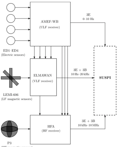
The scientific instrumentation aboard the RESONANCE spacecraft will include a particle and wave complex, amongst them low- and high-frequency electric field sensors – quasi-DC (direct current) to HF (high frequency). The high-frequency analyzer sensors (HFA) ranging from 10 Hz to 10 MHz and their supporting booms are analyzed in this project. The block diagram shown in Fig. 1 provides an overview of the instrument’s layout. HFA consists of cylin-drical sensors (so-calledB-antennas, labeled as ED1–ED4 in
Fig. 1) mounted on the tip of four boom rods (so-calledA
-antennas) which extrude from the central body of the space-craft. Furthermore, the boom rods themselves are used to-gether with the cylindrical sensors for mutual impedance measurements of the ambient plasma environment. The exact configuration is not yet completely fixed due to open ques-tions about the optimum arrangement, including electromag-netic as well as mechanical considerations.
2 Previous work and methods
In a related paper, Sampl et al. (2012), we already described the properties of the antenna system in the quasi-static fre-quency range, which were acquired by rheometry measure-ments and numerical computations. The herein presented computer simulations provide the characteristics of the an-tenna system from the quasi-static border up to 40 MHz, con-taining the proposed instrument’s operational range (up to about 10 MHz).
Numerical analysis of the sensor system for frequencies above the quasi-static regime provide the sought charac-teristics, where experimental techniques such as rheometry (Rucker et al., 1996; Oswald et al., 2009) or in-flight
calibra-ED1–ED4
(Electric sensors)
LEMI-606
(LF magnetic sensors)
P3
(HF magnetic sensors)
AMEF-WB
(ULF receiver)
ELMAWAN
(VLF receiver)
HFA
(HF receiver)
3E
0–10 Hz
3E + 3B
10 Hz–20 kHz
3E + 3B
10 kHz–10 MHz
SUSPI
Figure 1.Block diagram of the RESONANCE particle and plasma
wave complex.
tion (Vogl et al., 2004; Cecconi and Zarka, 2005) are prac-tically unfeasible. In the evaluation of spaceborne radio as-tronomy observations, the preferred quantity to describe the antenna is the effective length vectorhe. However, around
and above the first antenna resonance, this vector is intri-cate and cumbersome to use, because it becomes a complex-valued, direction-dependent quantity above the quasi-static frequency range (above some MHz).
θ
φ +Z
+X
+Y
Figure 2.Definition of spherical coordinatesθ (colatitude) andφ (azimuth) in the spacecraft-fixed reference frame as used for the representation of antenna axes.
Figure 3. Final, detailed patch-grid model of the RESONANCE
spacecraft, oblique view.
underlying electric field integral equation (EFIE) (Balanis, 2005) by applying the “method of moments” (MoM) (Mader, 1992). Using this method the EFIE is rewritten by expansion with a finite number of weighted basis functions into a sys-tem of linear equations, which can then can be solved by lin-ear algebra. More detailed solution approaches can be found in Harrington (1968), Wang (1990), and Schroth (1985) and respective literature.
3 Quantities for the characterization of the system
Above the quasi-static range the effective length vector changes with wave incident direction and frequency. Further-more, the sensor system is generally not purely capacitive anymore, so the impedance matrix cannot be represented in the form Z=(j ωC)−1 in terms of a real capacitance
ma-trix C. We therefore have to consider other parameters to quantify and illustrate the reception properties. For that pur-pose we use the antenna effective area and the elements of the impedance matrixZ. The former is always a real value,
−2 0 2 4 6 8 10
−0.5
0 0.5 1 1.5 2 2.5 3 3.5 4
+X Axis [m]
−2
−1
0
1
2
3
4
5
6
−2 0 2 4 6 8 10
+Z Axis [m]
+Y Axis [m]
cylindrical tip sensor (B3)
B3 A3
A1
A2
B4
A4 A3 A2
feed gap boom antenna (A3)
B1 B2
Figure 4.Final, detailed patch-grid model of the RESONANCE
spacecraft, top and front view.
whereas the latter is generally complex (with a purely imag-inary limit forω→0). We define the effective areaAof an
antenna as
A=|V|
2
|E|2, (1)
where V is the received voltage and E the electric field strength of the incident plane wave. Polarization matching is assumed, i.e., the conjugate ofEis proportional to the ef-fective length vectorhe, as defined by Macher et al. (2009).
This definition ofAis slightly different from the usual text
book definition (Balanis, 2005) and adapted to the measure-ment techniques and data evaluation methods applied in the present context, which rely on open-port voltages instead of power values. The usual definition refers to the received power per incident power flux (assuming polarization and impedance matching), which is of no use in the present con-text, it is even invalid for open ports.
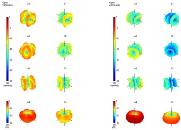
Figures 5 and 6 are dedicated to effective area patterns
Afor frequencies around the antenna resonances. The color
scale is logarithmic, with 0 dB at 500 m2for the upper three
patterns (A1–A3, B1–B3) and 0 dB at 50 m2 for the
low-est pattern (A4 and B4). With this normalization the
Figure 5.Effective area patterns of boom antennasA1–A4 and short cylindrical sensorsB1–B4 at 300 kHz (left) and 14 MHz (right).The panels show an oblique view, with the +xaxis pointing upwards, the +yaxis to the right and towards the observer, and the +zaxis to the right and away from the observer The color scale is at 0 dB/500 m2forA1–A3 andB1–B3 and at 0 dB/50 m2A4 andB4.
(A1–A3), so the ratio of the respective effective areas is about
a tenth, which explains the difference in the dB-reference val-ues (50 m2vs. 500 m2).
The first illustrated frequency is 300 kHz (Fig. 5, left panel), which is representative of the quasi-static range. We can clearly recognize the torus-like form of the patterns. The symmetry axes of the tori coincide with the directions of the respective quasi-static effective length vectors as shown in our related paper, (Sampl et al., 2012). The maximum ef-fective areas of theB-antennas are smaller than those of the A-antennas. We can verify this for thenth antenna boom by
calculating the ratio of the squares of the effective length vec-torshB
n andhAnby
max(ABn)
max(AAn)
=|hBn|
2
|hA
n|2
. (2)
This formula can be derived from the fact that the effective area is connected with the effective length vector via A= |e×h|2, with ebeing the unit vector pointing in the
direc-tion where the incident plane wave comes from. For instance, withn=1 we get the ratio max(AB1)/max(AA1)=0.31 in
the quasi-static range, using values from Table I in Sampl et al. (2012), which means a difference of about−5 dB be-tweenA- andB-antennas appearing in the color scale of the
patterns.
4 Sensor impedances
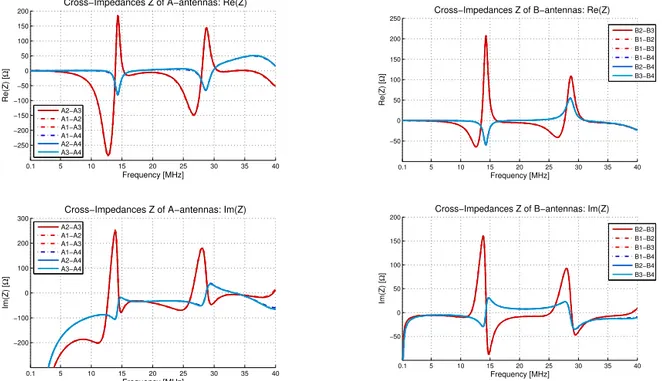
Figures 7 and 8 contain impedance curves, exhibiting the de-pendence of the elements of the impedance matrixZon fre-quency.
Figure 7 presents the (self-) impedances, i.e., the diagonal elements of the respective matrix, of theA- andB-antennas
(An−An andBn−Bn for n=1. . .4). Figure 8, left panel, is dedicated to the mutual impedances of A-antennas with
other A-antennas (An−Am for n, m=1. . .4 with n6=m). Figure 8, right panel, shows the corresponding curves forB
-antennas (Bn−Bmforn, m=1. . .4;n6=m). All other com-binations of mutual impedances/admittances of A-antennas
withB-antennas on the same boom (An−Bn) and on differ-ent booms (An−Bm; n, m=1. . .4;n6=m) are not shown, but can be found in Macher et al. (2009).
To show the antenna systems mutual impedances only one half of the off-diagonal elements of impedance matrixZneed to be depicted.Zis symmetrical due to the antenna systems reciprocity (Macher, 2012, 2014) and the other half gives the same curves again – apart from numerical inaccuracies. Many curves overlap due to the symmetry of the satellite ge-ometry; they are plotted in the same color.
In the impedance plots we recognize resonances at 14 and 28 MHz (q.v. Figs. 5 and 6), best visible as maxima in the real part in Fig. 7. They are very pronounced for the antennas
A1–A3 andB1–B3, but very faint if onlyA4 andB4 are
in-volved (ZA4,A4,ZB4,B4, andZA4,B4). These two resonances
appear at the frequencies where the boom length agrees with the half-wavelength (λ/2-resonance) and the full wavelength
(λ-resonance). Therefore, theλ/2-resonance associated with
the short boom (antennasA4/B4) can be expected at about 300
2·3.3≈45 MHz, where 3.3 m is the full boom length includ-ing mountinclud-ing. It is approached at the end of the exhibited frequency interval. Theλ/4-resonance associated with the
long booms is to be expected at about 4300·10.3≈7 MHz, and that of the short boom at 4300·3.3≈22 MHz. The displayed fre-quency interval contains only the first resonance (λ/4) for
the short boom, but it contains all the resonances up to the fifth (at≈35 MHz) for the long booms. The third and fourth resonance (≈21 MHz and ≈28 MHz) of antennas associ-ated with the long booms are more pronounced in the admit-tance plots. They are identifiable as zeros ofℑ(Z) in Fig. 7.
The reason for the deviation of the patterns from the respec-tive ideal dipole characteristic is the radiation coupling with the satellite body and also between the antennas. With the same reasoning we can see why it is plausible that theλ/
2-resonance of the long booms is split in two impedance max-ima.
In the mutual impedance (q.v. Fig. 8) and mutual admit-tance curves the resonances of both correlated antennas have their effect, so these curves are generally rather intricate. Even more since the real parts of the mutual impedances may be negative; actually they typically change signs close to the
λ/2 andλ-resonances (except forZAiBi;i=1. . .4). In
con-trast, the real parts of the self-impedances are always positive as they are representative of the power input to the antennas when operated in particular transmission modes.
5 Effective area pattern
Having identified the resonance frequencies, we can utilize this knowledge for a better understanding of the effective area patterns as shown in Figs. 5 and 6.
In the plots the principal axes are drawn in red (yaxis
par-allel toA1 andB1), green (zaxis) and blue (xaxis parallel to A4 andB4). The panels show an oblique view, with the +x
axis pointing upwards, the +y axis to the right and towards
the observer, and the +zaxis to the right and away from the
observer.
When we increase the frequency above the quasi-static range the toroidal shapes of the antenna patterns change. However, there is nearly no change of the shape up to 5 MHz, only the magnitudes increase. At 10 MHz the pat-terns get dented, but are still of toroidal shape. First we consider the antennas A1/B1–A3/B3. The closer the
fre-quency gets to theλ/2-resonance at 14 MHz (Fig. 5, right)
the more their pattern is changed, finally taking a com-pletely different form at the resonance frequency. Above theλ/2-resonance a pattern composed of two toroids
devel-ops (similar to an aircraft wheel), which remains up to the
0.1 5 10 15 20 25 30 35 40 100 200 300 400 500 600
700 Impedances Z of A−antennas − Re(Z)
Frequency [MHz] Re(Z) [ Ω ] A1 A2 A3 A4
0.1 5 10 15 20 25 30 35 40 −1000
−500 0
500 Impedances Z of A−antennas − Im(Z)
Frequency [MHz] Im(Z) [ Ω ] A1 A2 A3 A4
0.1 5 10 15 20 25 30 35 40 50 100 150 200 250 300 350
Impedances Z of B−antennas − Re(Z)
Frequency [MHz] Re(Z) [ Ω ] B1 B2 B3 B4
0.1 5 10 15 20 25 30 35 40 −4000 −3500 −3000 −2500 −2000 −1500 −1000 −500 0
Impedances Z of B−antennas − Im(Z)
Frequency [MHz] Im(Z) [ Ω ] B1 B2 B3 B4
Figure 7.Self-impedances of the boom antennasA1–A4 (left) and the short cylindrical sensorsB1–B4 (right). The shown quantities are the diagonal elements of the impedance matrixZas a function of frequency. Upper panels contain the real parts, lower panels the imaginary parts.
The curves for the boom antennasA1–A3 and sensorB1–B3 are nearly identical, which is due to the high symmetry of their deployment on the satellite.
0.1 5 10 15 20 25 30 35 40 −250 −200 −150 −100 −50 0 50 100 150 200
Cross−Impedances Z of A−antennas: Re(Z)
Frequency [MHz] Re(Z) [ Ω ] A2−A3 A1−A2 A1−A3 A1−A4 A2−A4 A3−A4
0.1 5 10 15 20 25 30 35 40 −200 −100 0 100 200 300
Cross−Impedances Z of A−antennas: Im(Z)
Frequency [MHz] Im(Z) [ Ω ] A2−A3 A1−A2 A1−A3 A1−A4 A2−A4 A3−A4
0.1 5 10 15 20 25 30 35 40 −50 0 50 100 150 200 250
Cross−Impedances Z of B−antennas: Re(Z)
Frequency [MHz] Re(Z) [ Ω ] B2−B3 B1−B2 B1−B3 B1−B4 B2−B4 B3−B4
0.1 5 10 15 20 25 30 35 40 −50 0 50 100 150 200
Cross−Impedances Z of B−antennas: Im(Z)
Frequency [MHz] Im(Z) [ Ω ] B2−B3 B1−B2 B1−B3 B1−B4 B2−B4 B3−B4
Figure 8.Mutual impedances of the boom antennasA1–A4 (left) and the short cylindrical sensorsB1–B4 (right). The shown quantities are the off-diagonal elements of the impedance matrixZ, as a function of frequency. Upper panels contain the real parts, lower panels the
Above theλ-resonance a transition region follows where the
pattern transforms into a shape composed of three toroidal lobes.
At theλ/2 andλ-resonance the antennas perform best in
the sense that they provide the highest gain in transmission mode and the highest sensitivity (with largest effective area) when receiving. But the quite irregular patterns at these res-onances do not admit an accurate prediction of the reception dependence on the direction of incidence, so direction find-ing is practically impossible at these frequencies. Off the res-onance frequencies gain and effective area are smaller but we can reckon with a rather regular pattern (as mentioned above a simple toroid or a shape composed of two or three toroids in the frequency range of interest). The mentioned λ/2 and λ-resonances are also visible in the effective area patterns of A4 and B4, causing a distortion of the toroidal form. The
ownλ/2-resonance ofA4/B4 antennas (≈45 MHz) distorts
their pattern at the end of the investigated frequency inter-val (40 MHz, Fig. 6, right), but is too far away to deform the toroid completely.
All investigations in this project are done for open ports, so it is assumed that the preamplifiers or receivers connected to the antennas have very high input impedances. If these impedances are not sufficiently high (of the order of 10 M
or higher) or cable capacitances are significant, one cannot speak of open-port operation anymore. In such a case the base impedances have to be taken into account. This can change the results significantly, in particular near the res-onance frequencies, as Gurnett et al. (2004), Macher et al. (2007) and Bale et al. (2008) have already shown in the con-text of former spaceborne antennas.
6 Conclusions
In this contribution we outline the properties above the quasi-static range of the space-borne electric field sensors as planned for the science mission “RESONANCE”. The re-ception patterns, self- and mutual impedances of boom an-tennas (A1–A4) and short cylindrical sensors (B1–B4) are
calculated from the results of numerical computations, cov-ering the whole instrument’s frequency range (from near DC to 40 MHz) with 100 kHz step size. Provided effective area patterns are of the typical toroidal shape in the quasi-static frequency range. The toroids get more and more distorted when increasing the frequency and adopt completely differ-ent, quite peculiar, shapes around the resonances. The pro-vided reception patterns give a visual estimate of the over-all reception properties, in particular how the effective areas, and the receiving sensitivity, of the antennas depend on the frequency and the direction of wave incidence.
Acknowledgements. The authors want to thank Mikhail Yanovsky
of the Russian Space Research Institute for the invaluable in-formation about the RESONANCE spacecraft design, and
Jean-Louis Rauch from the Laboratoire de Physique et Chimie de l’Environnement (CNRS) for information on the cylindrical tip sen-sors.
This work is part of the science project “RESONANCE electric field sensors: determination of the optimum configuration”, which was financed by the Austrian Research Promotion Agency (FFG) in the framework of ASAP 4, project 816159.
Edited by: V. Korepanov
References
Balanis, C. A.: Antenna Theory: Analysis and Design, John Wiley & Sons, Inc., Hoboken, New Jersey, USA, 3rd Edn., 2005. Bale, S., Ullrich, R., Goetz, K., Alster, N., Cecconi, B., Dekkali, M.,
Lingner, N., Macher, W., Manning, R., McCauley, J., Monson, S., Oswald, T., and Pulupa, M.: The Electric Antennas for the STEREO/WAVES Experiment, Space Sci. Rev., 136, 529–547, doi:10.1007/s11214-007-9251-x, 2008.
Boudjada, M., Galopeau, P., Mogilevski, M., Lecacheux, A., Kuril’chik, V. N., and Rucker, H.: RESONANCE Project: Com-parative studies of observational features associated to auroral radio emissions, in: The Inner Magnetosphere and the Auroral Zone PhysicsThe Inner Magnetosphere and the Auroral Zone Physics, Space Research Institute, Moscow, Russia, Moscow, 2010.
Cecconi, B. and Zarka, P.: Direction finding and antenna calibra-tion through analytical inversion of radio measurements per-formed using a system of two or three electric dipole antennas on a three-axis stabilized spacecraft, Radio Sci., 40, RS3003, doi:10.1029/2004RS003070, 2005.
Demekhov, A. G., Trakhtengerts, V. Y., Mogilevsky, M. M., and Ze-lenyi, L. M.: Current problems in studies of magnetospheric cy-clotron masers and new space project “Resonance”, Adv. Space Res., 32, 355–374, doi:10.1016/S0273-1177(03)90274-2, 2003. Gurnett, D. A.: Principles of Space Plasma Wave Instrument
De-sign, in: Measurement Techniques in Space Plasmas – Fields, edited by: Pfaff, R. F., Borovsky, J. E., and Young, D. T., Geo-physical Monograph, American GeoGeo-physical Union, Washing-ton, D.C., 1998.
Gurnett, D. A., Kurth, W. S., Kirchner, D. L., Hospodarsky, G. B., Averkamp, T. F., Zarka, P., Lecacheux, A., Manning, R., Roux, A., Canu, P., Cornilleau-Wehrlin, N., Galopeau, P., Meyer, A., Boström, R., Gustafsson, G., Wahlund, J.-E., Åhlen, L., Rucker, H. O., Ladreiter, H. P., Macher, W., Woolliscroft, L. J. C., Al-leyne, H., Kaiser, M. L., Desch, M. D., Farrell, W. M., Harvey, C. C., Louarn, P., Kellogg, P. J., Goetz, K., and Pedersen, A.: The Cassini Radio and Plasma Wave Investigation, Space Sci. Rev., 114, 395–463, doi:10.1007/s11214-004-1434-0, 2004.
Harrington, R. F.: Field computation by moment methods, Malabar, FL: Krieger, 1968.
Macher, W.: Inter-Reciprocity Principles for Linear
Network-Waveguides Systems Based on Generalized
Macher, W.: Transfer operator theory and inter-reciprocity of non-reciprocal multiport antennas, Progr. Electromag. Res. B, 60, 169–193, doi:10.2528/PIERB14051401, 2014.
Macher, W., Oswald, T., Fischer, G., and Rucker, H. O.: Rheometry of multi-port spaceborne antennas including mutual antenna ca-pacitances and application to STEREO/WAVES, Measure. Sci. Technol., 18, 3731–3742, 2007.
Macher, W., Sampl, M., Gruber, C., Oswald, T., and Rucker, H. O.: Resonance electric field sensors. Report on the ASAP4-Project, Technical Report IWF-183, Space Research Institute, Austrian Academy of Sciences, Austrian Academy of Sciences, Graz, Austria, 2009.
Mader, T.: Berechnung elektromagnetischer Felderscheinungen in abschnittsweise homogenen Medien mit Oberflächenstromsim-ulation, PhD thesis, Technische Universität Hamburg-Harburg, 1992.
McCormack, J.: Antenna Analysis: Antenna Scatterers Analysis Program, available at: http://raylcross.net/asap/ (last access: 8 September 2008), 1974.
Mogilevsky, M. M., Zelenyi, L., Trakhtengerts, V., Demekhov, A., Sukhanov, K., Sheikhet, A., Yanovsky, M., Romantsova, T., Rauch, J.-L., Parrot, M., F.Lefeuvre, Bosinger, T., Rietveld, M., Galeev, A., Burinskaya, T., Vaisberg, O., Smirnov, V., Nazarov, V., Kudryshov, V., Lichachev, V., Rusanov, A., Morozova, E., Savin, S., Sadovsky, A., Aleksandrova, T., Pasmanik, D., Baum, F., Kaurova, I., Batanov, O., Melnik, A., and Kharchenko, G.: Resonance Project. Study of wave-particle interaction and plasma dynamics in the inner magnetosphere. REPORT ON THE PHASE A., Tech. Rep. 54-R/26-2-131/R-E, Space Research Institute, 84/32 Profsoyuznaya Str., 117997, Moscow, Russia, 2002.
Mogilevsky, M. M., Zelenyi, L. M., Demekhov, A. G., Petrukovich, A. A., and Shklyar, D. R.: RESONANCE Project for Studies of Wave-Particle Interactions in the Inner Magnetosphere, Am. Geophys. Union, 199, 117–126, doi:10.1029/2012GM001334, 2013.
Oswald, T., Macher, W., Rucker, H., Fischer, G., Taubenschuss, U., Bougeret, J., Lecacheux, A., Kaiser, M., and Goetz, K.: Various methods of calibration of the STEREO/WAVES antennas, Adv. Space Res., 43, 355–364, 2009.
Rucker, H. O., Macher, W., Manning, R., and Ladreiter, H. P.: Cassini model rheometry, Radio Sci., 31, 1299–1311, 1996. Sampl, M., Macher, W., Gruber, C., Oswald, T., Rucker, H., and
Mogilevsky, M.: Calibration of Electric Field Sensors Onboard the Resonance Satellite, Antennas and Propagation, IEEE Trans., 60, 267–273, doi:10.1109/TAP.2011.2167918, 2012.
Schroth, A.: Moderne numerische Verfahren zur Lösung von Antennen- und Streuproblemen, Oldenbourg, 1985.
TU Hamburg-Harburg: CONCEPT-II, available at: http://www.tet. tu-harburg.de/concept, last access: 12 October 2010.
Vogl, D. F., Cecconi, B., Macher, W., Zarka, P., Ladreiter, H. P., Fedou, P., Lecacheux, A., Averkamp, T., Fischer, G., Rucker, H. O., Gurnett, D. A., Kurth, W. S., and Hospodarsky, G. B.: In-flight calibration of the Cassini-Radio and Plasma Wave Sci-ence (RPWS) antenna system for direction-finding and polariza-tion measurements, J. Geophys. Res. Space Phys., 109, A09S17, doi:10.1029/2003JA010261, 2004.