Summary —this article aims to explain the development of an application whose function is to predict the results of different sporting encounters. To do this an analysis of the influential factors, algorithms and technology implemented, will be carried out.
Key words — Bayesian Network, data mining, model of tasks and model of agents.
VI.INTRODUCTION
This research shows an early prototype based on Beliefs Networks, designed to provide the keys to be able to carry out a prediction of results for different sporting encounters, in our case a football match. For that purpose, we must analyse the different factors that form part of the information that determines the prediction:
• Climatic factors
• Ambient factors
• Human factors
Later on, the importance of variables such as humidity or temperature at the time the match is played and that of the stadium in which it is played, will be detailed. Besides this, how the state of the players, number of injured players etc will also be studied.
It is equally important to know the tools which will be used in the development of this prediction such as the probabilistic model (bayesian network and networks of Markov), the data minig or the different sources of data information to be analysed.
VII.BAYESIANNETWORKS
Everything related to bayesian networks can be found in references [1], [2] and [3].
A.Definition
A bayesian network is a structure which captures the existing dependency between the attributes of the observed data. The bayesian network describes the distribution of probability that governs the bringing together of the variables specifying suppositions of conditional independence along with conditional odds. Therefore the bayesian networks allow the specification of independent relations between the joining variables. Therefore, the network allows specific independent relationships between joining variables.
Between the characteristics of the bayesian network you can notice that they allow learning about dependant and casual relationships, to combine knowledge with data and can manage incomplete databases.
A bayesian network is a graph without cycle directed and
noted that describes the distribution of joint probability that governs an assembly of random variables.
So, a bayesian network B defines a unique distribution of joint probability:
It is important to observe the topology or structure of the network as it not only provides information about the probabilístics dependences between the variables, but also about the conditional dependencies of a variable or the joining those given or other variables. Each variable is independent of the variables that aren’t it’s descendants in the graph, given the state of their variable father.
The inclusion of the relationships of independence in the graphs’s structure makes the bayesian network a good tool for representing knowledge in a compact form (it reduces the number of parameters necessary). Besides this, it provides flexible methods or reasoning based on the propagation of the possibilities covering the network in agreement with the theory of probability laws.
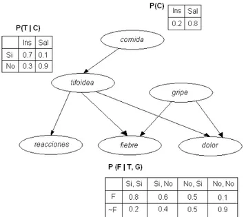
Figure 1 represents a specific example of a bayesian network which represents some knowledge about medicine. In this case the nodes represent illnesses, symptoms and factors that cause some illnesses. As mentioned previously, the variable which the arrow is pointing to depends on that which is in the origin. For example, fever depends on typhoid and flu.
It can be observed that the suppositions of wise independence can be observed by the network, for example, reactions depend on food, flu, fever and pain (nodes not descendant of reactions) given typhoid (it’s only node father). Therefore the following can be observed in the network:
P(R | C, T, G, F, D) = P(R | T)
Where R is reactions, C is food, T is typhoid, G is flu, F is fever and D is pain.
Also represented are the parameters of conditional probability associated with some of the network nodes. The table P(C) shows the values of probability previous to food consumption, P (T | C) the probability of typhoid given food consumed; and P (F | T, G) the probability of fever given typhoid and flu. In this case to record the parameters it isn’t necessary to maintain complete tables, given that the studied variables are binaries. As for each one it would only be necessary to record the values in a column. Taking into account that the size of the parameter tables grows exponentially with the number of fathers of a node, it is worthwhile recognising different techniques to reduce the number of necessary parameters.
B.Inference
Using the constructed network, and given the set values of some of the variables of an instance, it is possible to estimate the values of the other variables using probabilistics Kiyomi Cerezo Takahashi
reasoning.
The probabilistics reasoning through the bayesian network consists of spreading the effects of the evidences (known variables) through the network to learn of the probabilities after the unknown variables. This way, an estimated value for these variables un function of the probability values already obtained can de determined.
When the observed values are known for all the network variables except one, obtaining estimation for this is immediate from it formulates of the distribution of joint probability of the network.
In a more general case it would be interesting to obtain value estimation for a variable given the values observed for the subjoining of the remaining.
Different types of algorithms proposed exist, which are applied depending on the topology graph and obtain the probability of a single objective variable or of the entire unknown. It is not this projects intention to enter into details about different algorithms.
C. Learning about bayesian networks
The problem faced with bayesian learning can be described informally as: given the joining of training D = {u1, u2,..., uN} of instances of U, is found the network B which is better fitted to D. Typically, this problem can be divided into 2 parts:
• Structural learning: to obtain the network structure
• Parameter learning: knowing the graph structure, to obtain the probabilities corresponding to each node.
D.Parameter learning Complete data
Learning about the parameters is simple when all of the variables are completely observed together with the training. The most common method is the call estimator of maximum verisimilitude, which simply consists in estimating the
desired probabilities using the frequency of the training date values.
The quality of these estimations will depend on whether a sufficient number of samples. When this isn’t possible the existing uncertainty can be quantified representing it by means of a distribution of probability, thereby consider it explicitly in the definition of the odds. Habitually Beta distributions are employed in the case of binary variables, and distributions Dirichlet distributions for multi-value variables. This approximation is useful when counting on the support of the application experts to concrete the values of the distribution parameters.
Incomplete data
More difficulties surface when the training data is incomplete. 2 types of incomplete data are possible:
• Missing values: some missing values from one or various values in some examples
• Hidden Node: all of the variable values are missing
The first case is easier and various different alternatives exist:
• Eliminate the examples with missing values
• Consider a new additional value for the unknown variable
• Consider the most probable value using data from other examples
• Consider the most probable value based on the other variables.
The 2 first options are common with learning problems and always valid and there is a high number of incomplete data. The third option ignores the possible dependences of the variable, when the structure already counts the described graph, this doesn’t usually provide the best results.
The fourth technique serves for an already known network to infer the unknown values. Firstly, to complete the parameter tables using the all the complete examples. Then, for each incomplete instance, known values are assigned to the corresponding variables in the network and spreads it´s effect to retrospectively of those not observed. Afterwards, it is taken as the most probable observed value and all the probabilities of the model are updated before the following instance is processed.
The apparition of hidden nodes requires more complex treatment. In this case different techniques exist to estimate the missing values. One of the most common is the application of EM (Expectación Maximization). It’s application for the learning of parameters can be translated as the following:
• Assign random values (or values based on expert knowledge if available) to the unknown probabilities of the network.
• Use the known data to estimate unknown inferring them over the model with current probabilities.
• Complete a joining of data with the estimated values and then return to calculate the network probabilities.
• Repeat the two previous steps until there are no significant changes in the probabilities.
A certain similarity exists between the bayesian network learning when hidden nodes exist and the learning of weights in the hidden layers of a perceptron multilayered in which the values of entrance and exit for each sample are known, but no value for the elements of intermediate process. Based on this idea a graduating technique similar to that used in the algorithm of backpropagation. The technique intends to maximise the probability of the training data known the hypothesis P (D | h), considering the hypothesis joins all the possible combinations of the values for the odds that even customize curl the network. For this, follow the gradient in ln P (D | h) with respect to the network possibilities, updating every parameter wijk unknown in an interative way with the increase:
Where Wijk is the corresponding unknown parameter to the conditional probability of which the variable Xi takes the value Xij when it’s parents Πi take the values Πik, and k is a rate of learning. In each interaction the X probabilities re-stabilise after the increase.
The algorithm EM as well as the ascending gradient finds solutions which are only optimum locally, for which in both cases the quality of the result will depend on the initial assignation of the unknown probabilities.
Structural learning
Structural learning involves exploring a space of graphs. This task is very complex. When the number of variables (nodes) increases by a small amount the number of possible graphs constructed by them changes dramatically. Because of this on many occasions the search area for graphs is restricted by concrete characteristics. Many algorithms exist specifically for network learning where G is limited to a graph, or a multiple graphor to other less general structures.
Nevertheless, techniques exist to learn about networks with general structures, Working without restrictions should allow a construction of networks which fit better to the joinging of the training, for complexes that be the dependences among the attributes.
There are two approximations habitual for network learning when carrying out a guided search for an average global quality. The general operation consists of generating different graphs using a search algotihm and applying to each one of those a quality measuring function to decide which graph to save in every step.
Exist many algorithms that follow this technique, defined using by combining two elements:
• Search algorithm
• Global measure of adjustment
It is common to apply heuristics search algorithms. To try an exhaustive search over the graph space is simply intractable. Some of the possibilities are the assention techniques (hill climbing), genetic algorithms, bidireccionals, etc …another options is to apply a voracious search. It starts with an empty network to which successive local operations are applied improving by a maximal form the measurement of adjustment until an optimim local is found. The applied
operations incluyed the addiction, deletion and inversion of arrows.
Also there are many measurements of adjustment. Two common ones are the B measurements and and the description of the beginning of the minimum longitude.
The bayesian measurement intends to maximise the probability of the structure given the training data P (Bs | D). As the objective of the measurement is to compare the value obtained for different structures i and j, it is common the following quotient:
P (BSi | D) / P (BSj | D) = P (BSi, D) / P (BSj, D) Considering discreet variables and independent data, the joining probability of the second quotient can be estimated using the made predictions for each structure before the training data.
On the other hand, the main MDL characterises the learning in terms of undedrstanding the data. The objective of the learning is to find a model that aids the obtaining of the original data in the quickest way possible. Take into account the longitude of this description:
• The description of the model, penalising the complexity.
• The description of the data that the model used, encouraging their plausibility.
In the context of the bayesian network, the model is the network. Each bayesian network describes the conditional probability of PB above the instances that appear in the data. Using this distribution, a plan can be built and be codified that assign shorter words of code to the most probable instances. In agreement with the main MDL, a network B should be chosen such that the length combined of the description of the network and the data codified (with regard to PB) be low.
As from this point, different authors define different ways of measuring each element in the description using the general plan:
MDL (B | D) = complexity (B) – plausibility (D)
The bayesian as well as the MDL are both well known and well studied. Both function are asymptotic equivalents when the size of the sample is increased, and besides this the correct asymptotic: With probability equal to one the distribution learned converges to the underlying distribution
to the extent that the number of sample enlarges.
VIII.MARKOVNETWORKS
According to [1] A network of Markov is a pair (G, Ψ) where G is a graph done not direct Ψ = {ψ1(c1), . . . , ψm(cm)} Is an assembly of potential functions you defined in the conglomerates C1, . . . , Cm of G that define a function of probability p (x) by middle of
.
If the graph done is not direct G is triangulated, then p (x) can also be factorized, utilizing the functions of probability conditioned P = {p (r1|s1), . . . , p (rm|sm)}, of the following form
Where Ri and If are the residues and separators of the conglomerates. In this case, the network of Markov comes given by (G, P). The graph G is an I-MAP done not direct of p (x).
Therefore, a network of Markov can be utilized to define the qualitative structure of a model by means of the factorization of the function of corresponding probability through potential functions or functions of probability conditioned. The quantative structure of the model will correspond to the concrete numeric values assigned to the functions that appear in the factorization. All of this is reflected in [4].
IX.DATAMINING
Leaving from the article [5], date mining came about as a technology which would try to aid the comprehension of the contents of a database. In a general way, the data is the prime material. In the moment the user attributes an especial significance it become information. When the specialists elaborate or find model. Doing the joined interpretation between information and this model represents an aggregate value, and then we refer to knowledge. Figure 2 shows the hierarchy that exists in a database between data, information and knowledge. Also observed is the volume present in every level and the value that those responsible for the decisions give to this hierarchy. The area inside the triangle represents the proposed objectives. The separation of the triangle represents the long union between data and information, but not between the information and knowledge. The data mining works in the superior level looking for XX, behaviour, grouping, sequences, trends or a associations that can generate a model that allows us to understand better the dominium to help in possible decision making.
Reflecting on the previous text we can say that Datamining is the process of discovering patterns of interesting and potencially useful information, immersed in a big database which is constantly interacted with. Datamining is a combination of processes such as:
• Extraction of data
• Data cleaning
• Characteristic selection
• Algorithms
• Analysis result
The usefulness of data mining can be given inside the following aspects:
The usefulness of data mining can be given inside the following aspects.
• Systems partially unknown, if the system model that produces the data is well known, then we don’t need the data mining as all of the variables are predictable. This is not the case in commercial electronic, due to the effects of human behaviour and climate. In these cases there will be a part of the system which is known and there will be a part altered by nature. Under these circumstances, starting from a large amount of data associated with the system, the possibility exists to find new aspects previously unknown to the model.
• Large amounts of data: to find a lot of information in some databases is important for a company to find the form of analising “mountain” of information (which for a human is impossible) and that is prove some type of result.
• Potent hardware and software: Many of the present tools in the mining industry of data are based on the intensive use of the computation, consequently, a convenient team and an efficient software, with which count a company, will enlarge the performance of the process to seek and to analyze information, which at times should turn them with productions of data on the order of the Gbytes/Hour The use of the dates mining can be beneficial Possessing data on its productive processes, clients monitoring data, etc.
The general phases for the creation of a data mining industry project independently of the technique specifies of extraction of know-how used:
• It Filtered of data: The format of the contained data in the source of data never is the suitable one, and the majority of the times is possible to utilize no algorithm of mining industry. By means of the preprocessing, the data are filtered (are eliminated unknown, invalid, incorrect values, etc.), samples of the same are obtained (greater velocity of answer of the process), or they are reduced the number of possible values (by means of I round, grouping, etc.).
heuristics algorithms.
• Extraction of know-how: By means of a technique is obtained a model of knowledge, that represents bosses of behavior observed in the values of the variables of the problem or relations of association
among variable happinesses. Also they can be used several techniques at the same time to generate different models.
• Interpretation and evaluation: Finally it proceeds to their validation, verifying that the conclusions are valid and satisfactory. In the case of to have obtained various models by means of the use of different techniques, the models in search should be compared of that that be adjusted better to the problem. If none of the models reaches the results expected, some of the previous processes in search of new models will be altered.
X.FACTORSTHATINFLUENCETHEANALYSIS
A.Climatic factors
To all lights we can affirm that the importance of the climatic situation during the celebration of a sports event that is disputed outdoors is determinant in the analysis of the possible results.
There it will be that to be keep in mind factors as the rain, snow, if this cloudy or sunny in the same way that the temperature and the humidity that there is at the moment to dispute the party. All these variables should be quantified at the moment of to do the calculations of the odds that were used to do the prediction.
B.Human factors
In whichever sport the most influencial factor is the human factor and because of it one must treat to quantify variables as the so much state of mind like the physicist since both are influential at the moment of to carry out a sport. Besides it is necessary to know the state of the team as important assembly being to know the possible drops that has a team, quantifying the shrinkages that produces in the possibilities of winning a match.
XI.APPLICATIONDESIGN
According to the following plan:
The operation of the application itself B utilizing an agent of natural language that is reached by Internet, to them you paginate sports, where by means of a web semantics and a meticulous one ontology would be obtained and storing the necessary key information for our prediction.
On the other hand another agent, the meteorologic access to the National Institute of Meteorology by means of the same mechanism that the agent of natural language to collect and to store the referring information to the cities where the sporting events were celebrated.
Once they executed these two agents should act the filter agent, which takes charge of filtering and store information that is not prominent and also has been stored for the agent of natural language.
After this moment the application executes the agent of inference responsible that utilizes all information filtered and the climatic data to apply them a series of rules based on the networks B, to foretell with accuracy and truthful.
One intelligent agent finalizes the execution of all inference task, the interface agent takes charge of showing this information to the user whether computer or any mobile device.
To develop the application a tool is used for Bayesian Network creation that determines this work, Genie 2.0, diagram below shows it´s construction
Once the bayesian netwok is designed we should use an API to be able to use it in the implementation of the program code Java in which we have done the application. The API is jSmile, a wrapper that should be added to the project as a bookstore.
Following we must use a database; in our case we will use Access since we do not need the boards to be very complicated. We will have a board with the parties of the day, another with the meteorological information, on each team of the day and to finish one with all fields that are defined within bayesian network structure.
How the application works?
The program is based on an application web in which we will be able to agree as administrator or client.
If login as client, the user can see a listing with all matches
Fig. 4. Bayesian Network
Administrador
Internet
Agente ALN
Servidores
Agente Meteorologico
Agente de filtrado
Agente de inferencia
Agente de interfaz
Miembro
that are disputed in that day. The user should select the match that desire to visualize the prognostic so the application carry out the inference of the database with the information stored previously.
In the case that it be agreed as the administrator itself will have access to several options, such as access to meteorological information, which has been collected by the National Institute of Meteorology or to the referring information to all teams of football that has been collected from main sports pages of the network by natural language agents
In this section the administrator should filter some information collected since not all the information is relevant. This procedure avoids redundancies.
XII.CONCLUSIONS
After execution of a complete battery of tests, we have been verified that there are not sufficient variables. The ones that have kept in mind themselves are the human aspects, (difficult to measure of an objective form) and climatic factors (do not affect equally to all the teams). Because of that, our prototype should be worked using real-time data (climate, people) as statistics (historic) to improve our inference process. Web Service technology and SOA world provides new scenarios that suggest the possibility to improve our early Bayesian inference process.
REFERENCES
[1] Enrique Fernández. Análisis de clasificadores bayesianos [on line].
Facultad de Ingeniería de la universidad de Buenos Aires. Disponible en: http://www.fi.uba.ar/materias/7550/clasificadores-bayesianos.pdf.
[2] Nir Friedman. Bayesian Network Classifiers [on line]. Cop. Kluwer
Academic Publishers, Boston. Disponible en: http://www.cs.huji.ac.il/~nir/ Papers/FrGG1.pdf
[3] G. Cooper(1990). Computacional complexity of probabilistic inference
using bayesian belief networks (reserch note). Artificial Intelligence, 42, pp 393-405.
[4] Enrique Castillo, José Manuel Gutiérrez, Ali S. Hadi. Sistemas expertos y
modelos de redes probabilísticas. Pp 207-241.
[5] Luis Carlos Molina. Universitat Politecnica de Catalunya. Articulo: “Data