www.ocean-sci.net/12/1249/2016/ doi:10.5194/os-12-1249-2016
© Author(s) 2016. CC Attribution 3.0 License.
GEM: a dynamic tracking model for mesoscale
eddies in the ocean
Qiu-Yang Li1, Liang Sun1,2, and Sheng-Fu Lin1
1School of Earth and Space Sciences, University of Science and Technology of China, 230026, Hefei, China 2State Key Laboratory of Satellite Ocean Environment Dynamics, Second Institute of Oceanography, State Oceanic Administration, Hangzhou, 310012, China
Correspondence to:Liang Sun ([email protected])
Received: 21 June 2016 – Published in Ocean Sci. Discuss.: 13 July 2016
Revised: 10 November 2016 – Accepted: 11 November 2016 – Published: 2 December 2016
Abstract. The Genealogical Evolution Model (GEM) pre-sented here is an efficient logical model used to track dy-namic evolution of mesoscale eddies in the ocean. It can dis-tinguish between different dynamic processes (e.g., merging and splitting) within a dynamic evolution pattern, which is difficult to accomplish using other tracking methods. To this end, the GEM first uses a two-dimensional (2-D) similarity vector (i.e., a pair of ratios of overlap area between two ed-dies to the area of each eddy) rather than a scalar to mea-sure the similarity between eddies, which effectively solves the “missing eddy” problem (temporarily lost eddy in track-ing). Second, for tracking when an eddy splits, the GEM uses both “parent” (the original eddy) and “child” (eddy split from parent) and the dynamic processes are described as the birth and death of different generations. Additionally, a new look-ahead approach with selection rules effectively simplifies computation and recording. All of the computational steps are linear and do not include iteration. Given the pixel num-ber of the target regionL, the maximum number of eddiesM, the numberNof look-ahead time steps, and the total number of time stepsT, the total computer time isO(LM(N+1)T ). The tracking of each eddy is very smooth because we require that the snapshots of each eddy on adjacent days overlap one another.
Although eddy splitting or merging is ubiquitous in the ocean, they have different geographic distributions in the North Pacific Ocean. Both the merging and splitting rates of the eddies are high, especially at the western boundary, in currents and in “eddy deserts”. The GEM is useful not only for satellite-based observational data, but also for numerical simulation outputs. It is potentially useful for studying
dy-namic processes in other related fields, e.g., the dydy-namics of cyclones in meteorology.
1 Introduction
Eddies are ubiquitous in the ocean, and they move from one place to another (Chelton and Schlax, 1996; Chelton et al., 2007). Eddies in the ocean can cause large-scale transports of heat, salt, and other tracers (Bennett and White, 1986; Chelton et al., 2011a; Dong et al., 2014; McGillicuddy et al., 2011) by trapping these passive tracers inside the eddies. Such transports may have important impacts on the environ-ment and climate of the ocean (Dong et al., 2014). To address various applications in the studies that use satellite products of sea level anomaly (SLA) data (e.g., Chelton et al., 2011b) and numerical simulation outputs (e.g., Petersen et al., 2013), oceanic eddies should be automatically recorded using these data and outputs (e.g., Yang et al., 2013; Sun et al., 2014; Pegliasco et al., 2015). In general, the recording of oceanic eddies often includes two independent steps: automated eddy identification and automated eddy tracking. The eddies are identified in a sequence of SLA maps using an identification algorithm or identified from velocity fields. An automated tracking procedure is then applied to determine the trajec-tory of each eddy (Chelton et al., 2011b). Several automated identification and tracking algorithms have been developed for eddies in the ocean (Chelton et al., 2011b; Ienna et al., 2014; Mason et al., 2014; Yi et al., 2015).
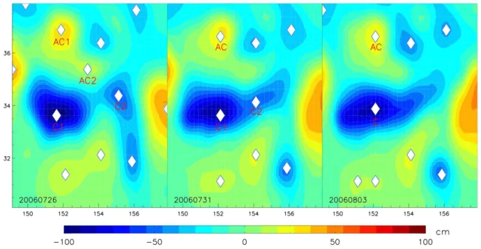
Figure 1.The evolutions of amplitudes and areas of eddies from 5 July to 3 August 2006 (after Li et al., 2014), where the background field shows the SLA, and white dots mark eddy centers. Two anticyclonic eddies AC1 and AC2 merged into a single eddy on 31 July 2006, and two cyclonic eddies C1 and C2 merged into a single one on 3 August 2006.
of eddies may be found in proximity to a neighboring eddy in any given global SLA map, and they frequently interact. Therefore, an eddy tracking process should have the capabil-ity to distinguish between different dynamic processes (e.g., merging and splitting) during its dynamic evolution. More-over, an eddy tracking process must be accurate and fast enough to handle a huge amount of data, which will be even larger in size if the spatio-temporal resolution of observations and numerical simulations increases.
Implemented automated tracking procedures differ in de-tail, but they are all similar in concept because they utilize the nearest neighbor strategy (Chelton et al., 2011b). For each eddy Ei identified at time stepk, the nearest eddy toEi at the next time stepk+1 is identified as part of the trajectory of eddyEi. A more advanced procedure uses eddy shape error as an additional condition when assessing an eddy trajectory (Mason et al., 2014).
However, there is a “missing eddy” problem that must be solved in the eddy tracking stage (Chelton et al., 2011b). An eddy at time step k may have no associated eddy at time stepk+1, which is simply due to a temporary missing eddy
in the identification process; this can occur for a variety of reasons related to sampling errors and measurement noise (Chelton et al., 2011b) or limitations of the eddy detection step when an eddy is too weak/small at a time step. Chelton and his colleagues made an attempt to accommodate such problems; they allowed for the reappearance of a temporarily missing eddy by looking ahead two or three time steps. Un-fortunately, this “look-ahead” procedure considers too many
nearby eddies as potential ones. In practice, the results of this simple “look-ahead” procedure were disappointing be-cause the resulting eddy trajectories often jumped from one eddy track to another. As a result, the look-ahead approach was abandoned, even though it is a solution to the “missing eddy” problem (Chelton et al., 2011b).
Recently, the concept of multiple hypothesis assignment (MHA) was introduced to solve the missing eddy problem by abandoning the simple closest eddy strategy and applying a new “look-ahead” procedure (Faghmous et al., 2013). The MHA method can effectively solve the missing eddy problem in a straight-line model when the trajectory being followed is a branch without any splitting, but it is algorithmically and computationally complex. Given the maximum number of eddies in any time frameM, the number of look-ahead time stepsN (withN=0 being the original linear closest eddy procedure without look-ahead), and the total number of time stepsT, the MHA has a larger computer time (the total amount of time taken by an algorithm),O(MN+1T )in the worst case (Faghmous et al., 2013).
on 31 July 2006. Then, the cyclonic eddies C1 and C2 on 26 July 2006 merged to form a larger one on 3 August 2006. To describe such processes, the eddy tracking records should be trees with branches instead of simple straight lines.
To record the dynamic evolution of eddies, two funda-mental algorithms are required. First, the two nearby eddies should be distinguished in the identification stage using a segmentation strategy in which the target region is divided into two corresponding eddies. Otherwise, the merging and splitting processes cannot be determined properly. This prob-lem was recently solved by the use of segmentation strate-gies, e.g., the close-distance segmentation strategy (Li et al., 2014) and the watershed strategy (Li and Sun, 2015). Be-cause these segmentation strategies can distinguish between closed eddies, they can also potentially reduce the risk of missing an eddy in the identification process.
Second, the merging and splitting processes in the track-ing stage should be described in detail. We use a multi-branch tree model to do so. The eddyEiidentified at time stepkmay arise from two or more eddies (at time stepk−1), which sub-sequently merged, andEi may become more than one eddy at time stepk+1 if it splits. We refer to this model as the Ge-nealogical Evolution Model (GEM) because it is a genealog-ical tree for recording the whole evolutionary history of an eddy. The multi-way tree model in computer science can be used to store this type of structure.
Moreover, the GEM also provides a new way to solve the missing eddy problem. Instead of the existing closest eddy strategy, a temporal track tree withN look-ahead time steps is used to maintain all possible tracks with the help of the multi-way tree model. The method can effectively solve the missing eddy problem, regardless of whether the eddy is splitting or not.
In this paper, we introduce the GEM to describe mesoscale eddies in a tracking process with a total number of time steps T. The GEM allows the eddy to have multiple eddies as its parents or as its children in a multi-branch model. It also solves the missing eddy problem by using a new look-ahead method similar to the MHA. Compared with the computer timeO(MN+1T ) of MHA, the new method is much faster and has much less computer time O(LM(N+1)T), where L denotes the number of pixels of a target region. Besides, if the GEM was implemented with the computer codes prop-erly, the output data of the GEM also record the dynamic evolution of the eddy in detail and will potentially be useful for other research fields, e.g., the dynamics of cyclones in meteorology. As an example, the GEM is applied to eddies in the North Pacific Ocean (NPO) only, and we assume the eddies do not cross the Equator.
The paper is organized as follows. The data and eddy de-tection methods used in this study are introduced in Sect. 2. Then the GEM is introduced in Sect. 3, including a simi-larity vector, a look-ahead approach and the worst-case run-time. Results including eddy tracks and examples of merging and splitting events in a sample area in the North Pacific are
shown in Sect. 4. The impacts of data noise and parameter uncertainties on the results are discussed in Sect. 5. Finally, a summary and conclusions are given in Sect. 6.
2 Eddy identification 2.1 Input data
The input data consist of the original altimetry field, which can come from satellite observations or numerical simu-lations. The altimetry field used in this study is the 20-year (1993–2012) daily SLA data from the merged and gridded satellite product of Maps of Sea Level Anomaly (MSLA) at 0.25◦×
0.25◦
resolution in the global ocean from AVISO (http://www.aviso.oceanobs.com/). In this study, we use the “DT14” (delayed-time 2014) altimeter product (Du-acs/AVISO, 2014), which is adequate for direct eddy detec-tion (Capet et al., 2014), though it still has about 2–3 cm er-ror globally for short temporal scales (Carrere et al., 2016). A comprehensive discussion of gridded AVISO products for eddy investigations can be found in Chelton et al. (2011b).
We used the original SLA data (“DT14”) without any fil-tering or smoothing to identify eddies in this study. However, this does not imply that data smoothing is not needed for the SLA data in related studies (e.g., eddy detection, eddy tracking). For example, to calculate some eddy parameters (e.g., velocity and vorticity), smoothing may be required, as pointed out by Chelton et al. (2011b). Moreover, the data er-rors, even if they are very small, might affect the eddy detec-tion (see the discussion in Sect. 5.1).
2.2 Eddy identification
The eddy identification used in this study is similar to those used before (Chelton et al., 2011b; Mason et al., 2014) to identify eddies from SLA data. The eddies may be identified as multinuclear (two or more SLA extremes in one eddy) or mononuclear (only one SLA extremum in one eddy). The fol-lowing mononuclear eddy definition is also similar to what was used by other authors (Chaigneau et al., 2011; Li et al., 2014; Li and Sun, 2015). We have adopted the eddy detec-tion step from Li and Sun (2015), which provides us with the necessary input for the tracking routines, namely eddy areas and boundaries. Each pixel has eight nearest neighbors. A point within the region is a local extremum if it has an SLA greater or less than all of its nearest neighbors. We also use such a definition of an extremum in our following analysis, in which the extrema are identified by checking each pixel in the map along with the 8 pixels around it. An eddy is defined as a simply-connected set of pixels that satisfies the follow-ing criteria.
1. The SLA value of all of the pixels is above (below) a given SLA threshold.
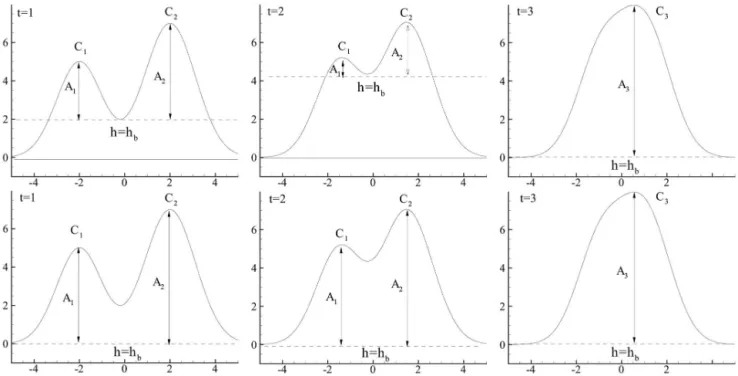
Figure 2.Top panels: time evolution of two merging eddies revealed by the mononuclear eddy identification without segmentation. Bottom panels: time evolution of two merging eddies revealed by the mononuclear eddy identification with segmentation. The hrepresents the background SLA value,Arepresents the amplitude of the eddy, andtrepresents the map at different times.
3. The amplitude of the eddy (the max difference of SLA values) is larger than a critical value (e.g., 1 cm). 4. The area of the eddy must be large enough for
estimat-ing eddy parameters (say > 16 pixels).
Conditions 3–4 provide the lower bounds for eddy size and amplitude. These conditions automatically reduce the total number of detected eddies. Condition 1 is the same as the first criterion in Chelton et al. (2011b). It is used in consideration of the 2–3 cm of background SLA error (Carrere et al., 2016); so, small fluctuations in SLA field would not be taken as ed-dies in this study. Condition 3 was generally used previously (Chaigneau et al., 2011; Chelton et al., 2011). Condition 4 is more restrictive than the generally used value of 8 pixels (e.g., Chelton et al., 2011; Li et al., 2014); so, this condition is an add-on, which is potentially useful when deriving eddy parameters using a nonlinear optimal fitting method (Wang et al., 2015; Yi et al., 2015). If the eddy area is too small (only a few pixels), its parameters (e.g., amplitude, area, radius) are very sensitive to its area (number of pixels). Besides, we do not put limits on eddy pixel number maximum (e.g., < 1000) and eddy size (e.g., < 400–1200 km), while such limits were generally used previously (e.g., Chelton et al. 2011; Mason et al., 2014).
The SLA extremum so determined is called the eddy cen-ter. The set of pixels belonging to an individual eddy is re-ferred to as the area of the eddy, and the outmost SLA contour is the boundary of the eddy. We use the area and boundary to calculate the similarity of eddies in Sect. 3.2.
Each eddy is identified by the following procedures. First, according to condition 1, we find a simply-connected region with a given threshold of SLA <−3 cm for cyclonic eddies and SLA > 3 cm for anticyclonic eddies. Second, we check whether there is at least one extremum in the region. If the eddy is multinuclear, we use a segmentation method to seg-ment them to satisfy condition 2. Finally, we check whether the region satisfies the eddy conditions 3 and 4; we remove weak (amplitude < 1 cm) and small (pixels < 16) eddies.
2.3 Eddy segmentation for merging and splitting events Figure 2 illustrates the necessity for eddy segmentation based on the merging process of two eddies. Different mononu-clear algorithms are used in the upper and lower rows. In the top panels of Fig. 2, eddies are identified by the non-segmentation algorithm. Such mononuclear eddies may be very small. The time evolutions fromt=1 tot=3 show a
al-gorithm (Li and Sun, 2015). During the time from t=1 to t=2, both their amplitudes and areas are only marginally changed, while their distance is continually reduced. Then, a large eddy C3 naturally emerges in the same region, while C1 and C2 disappear. It is recognized from the eddy data that C3 is the merging result of C1 and C2.
Figure 3 illustrates this eddy segmentation strategy. Fig-ure 3a shows two individual but nearby eddies. The pixels between the two dashed lines are naturally divided by the watershed (For basins, the “watershed” is a ridge between them, while it is a valley for plateaus.) As shown in Fig. 3b, the cross section of the eddy clearly shows that two closely located pixels P1 and P2 on the left and right sides of wa-tershed would slide along the path of steepest descent in the map of SLA data to different eddy centers. The shape of SLA can provide sufficient information to segment the multinu-clear eddy into mononumultinu-clear ones.
Herein, we use the mononuclear eddy identification (MEI) of the Universal Splitting Technology for Circulations (USTC) with watershed segmentation (Li and Sun, 2015) and include in our code the calculation of eddy parameters, in-cluding amplitude, radius, area, and boundary (Fig. 3), which might be potentially used in other studies (Sun et al., 2014).
The output eddy parameters from MEI are then used as in-put for our novel tracking algorithm GEM. The GEM mainly represents the logical relationship of eddies, which is less de-pendent on physical parameters which may change greatly because of dynamic evolution (e.g., splitting, merging). To this end, the GEM takes the previously identified eddies by MEI (with area/boundary; see Sect. 2.2) as its input data.
3 Dynamic tracking 3.1 Overview of the GEM
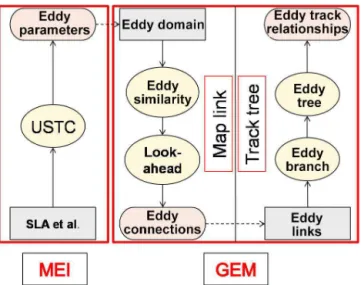
The GEM is a logical model used for tracking the dynamic evolution of mesoscale eddies in the ocean (Fig. 4). The model essentially establishes logical relationships of previ-ously identified eddies. The relationships are determined by two relatively independent steps; i.e., the GEM algorithm consists of two parts (see Fig. 4 for details): first, measuring the “map link” between two time steps, and then connecting all time steps to the “track tree”.
The first part of the GEM is “map link”, which uses as in-put eddy data obtained in the prior eddy identification step (area/boundary; see Sect. 2.2) to establish the link of an eddy from one temporal snapshot to the next, namely living, miss-ing, death, birth, and the associated dynamical processes of merging and splitting. In this part of the work flow, we use a 2-D vector rather than a passive scalar to measure the similar-ity between eddies E1 and E2 on 2 neighboring days (Figs. 5 and 6; see Sect. 3.2.1 for details). We then use a relatively complex look-ahead procedure to solve the missing eddy problem (Sect. 3.2.2). This new look-ahead approach has a
duration ofNdays (Fig. 7). Finally, the links of the eddies in different snapshots are saved (see Sect. 3.2.2 for details).
The second part is “track tree”, which uses the outputs from “map link” (i.e., eddy links) as its input (Fig. 4). It connects the eddy links from branches to a tree with the ge-nealogical model (Fig. 8) using two sub-procedures: “eddy branch” and “eddy tree”. In the “eddy branch” part, we use parentandchildto define the eddy relationship and define all possible types of eddy states: birth, death, living, miss-ing, mergmiss-ing, and splitting (Fig. 8a). Consequently, we iden-tify different roles in the eddy branches (see Sect. 3.3.1 for details). Finally, in the “eddy tree” procedure, we connect the branches based on their roles (parent, child, and grand-child, etc.) in the genealogical tree (Fig. 8b). The output of the GEM includes eddy tracks and the records of eddy rela-tionships (see Sect. 3.3.2 for details).
In short, the GEM uses previously identified eddies and/or their links to make dynamic tracks via a genealogical tree model. In addition to eddy domain and boundary, it needs two parameters as input, the critical value of area ratiorc andN. See Sect. 5.2 for a discussion on the impacts of these parameter choices.
3.2 Map link
To establish the relationships between the previously iden-tified eddies, the first part of the GEM used evaluates the similarity of these eddies, which is defined here based on the overlap of the domain of an eddy in two consecutive time steps. It begins with defining similarity based on the overlap-ping area of eddies in consecutive time steps. Subsequently, the overlapping area which is closest to the one of the orig-inal eddy is defined to be the successor of the origorig-inal eddy (if the threshold is met).
3.2.1 Eddy similarity
At first, the eddy similarity is calculated with an exam-ple (Fig. 5a) before proceeding to the mathematical expres-sions. There were three eddies A1, A2, and B1 detected on 28 March 1997. In Fig. 5b, there were four eddies A1, A2, B1, and B2 on 29 March 1997. We overlapped the eddy do-mains into a single map (Fig. 5c). Then, we used the inter-section of eddy domains on different days to calculate the similarity. For eddies A1 and A2, the intersections were very close to their respective domains on 28 and 29 March. For eddy B1, the intersection was close to the area on the second day, but it was only part of that on the first day. Consequently, eddies A1 and A2 had full similarity on these days, while ed-dies B1 and B2 only had partial similarity on these days.
Figure 3. (a)Watershed as the natural division of eddies C1 and C2 from the top view, where contours represent SLA.(b)The particles P1 and P2 on the watershed flow downward to the eddy centers C1 and C2 from the cross-section view. After Li and Sun (2015).
Figure 4.Flowchart of the systems. Mononuclear eddy identifica-tion (MEI) uses SLA to identify eddies via the Universal Splitting Technology for Circulations (USTC) method. The GEM, which has the two independent parts of “Map link” and “Track tree”, then uses the previously identified eddies for tracking.
that are identified in the same region on day 1. This compari-son region, which is centered at the eddy center of E1, moves in time with the target eddy (E1). To determine the
similari-ties between E1 on day 0 and E2 to E4 on day 1, we intersect the domains of day 0 and day 1. For example, to determine the similarity between E1 and E2, we count the overlap area S12 (defined as the intersection of Boundary 1 and Bound-ary 2) between E1 (areaS1) and E2 (areaS2), and then we calculate the following ratios:
r1=S12/S1, (1a)
r2=S12/S2. (1b)
Clearly, the values ofr1andr2are within (0, 1). The larger r1 andr2are, the larger the probability that E2 will be the snapshot of E1 on day 1. Eddy movement speeds are gener-ally less than 0.1 m s−1, which implies that an eddy can only move one grid box (0.25◦) in 3–4 days. Thus, the overlap on
different subsequent days of the same eddy area should be large enough. This is one of the parameters to set. When we apply the GEM to track eddies in the North Pacific Ocean (Sect. 4.1), we chooserc=2/3, and the choice ofrcis com-prehensively addressed in Sect. 5.2.
Figure 5.Sketch of eddy overlaps.(a)The SLA map (shading) and the boundary of eddies (red curves) on 28 March 1997, where A1, A2, and B1 represent identified eddies.(b)The SLA map (shading) and the boundary of eddies (blue curves) on 29 March 1997.(c)The intersection of eddy areas by overlap eddy identification maps.
Figure 6.Sketch of eddy similarities.(a)The sketch of eddy overlaps. Eddy E1 (black) is the eddy identified on day 0, where the thin contours represent the eddy parameter (e.g., the SLA value). The thick contour represents the eddy boundary. Eddies E2 (blue), E3 (green), and E4 (red) are identified on day 1. We consider the overlap between the two eddies on different days to evaluate the similarity between them.(b)There are four similarity types (T0–T3) according to the values ofr1,r2, and the critical valuerc; there is at most one eddy that can be marked as a T1 (merging) or T3 (living) eddy on the following day.
(T1: r1>rc and r2<rc), where E1 on day 0 is part of E2 on day 1 (E1 enlarging or merging); Type 2 (T2:r1<rcand r2>rc), where E2 on day 1 is part of E1 on day 0 (E1 decay-ing or splittdecay-ing); and Type 3 (T3:r1>rcandr2>rc), where E1 and E2 are the same eddy at different locations on differ-ent days (E1 living and moving). The last type (T3, living) is prescribed in cases when the center of E1 propagates less than a pixel toward that of E2, because the eddy movement speed is physically less than one grid (0.25◦
) per day. For example, eddy B1 on 29 March 1997 in Fig. 5b is simply assigned to T3 (living) even though r1<rc. Eventually, we
obtain the relationships between E1 and E3 or E4 (Fig. 6a). Because the present method uses a vector to express eddy similarity, we call it the similarity vector. This is an alterna-tive to scalar similarity parameters (e.g., Ienna et al., 2014; Mason et al., 2014).
Figure 7. (a)Three typical cases of successors (T1, T2, and T3) from one day (day 0) to another (day 1).(b)The eddy at day 0 may have different successors corresponding to different numbers of “look-ahead” days; e.g., Ed1 at day 0 may have a T3 eddy on day 2 and have two T2 eddies on day 3.
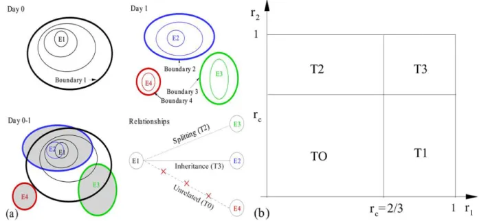
Figure 8. The logical genealogy of an ocean eddy with six states: birth, death, living, missing, splitting, and merging.(a)The logical relationships of eddies between 2 days.(b)The logical genealogy evolution model of an example eddy.
the overlap in their areas is small or zero. In other words, their overlap rates are below the critical valuerc(marked as T0 in Fig. 6).
In previous eddy tracking studies, simple methods were used for weekly SLA data (delayed-time 2010), e.g., the closest distance between eddies (Chelton et al., 2011b; Yi et al., 2015), the closest angle between eddies (Zhang et al., 2014), and the dimensionless similarity scalar (Chaigneau et al., 2008; Mason et al., 2014). There is always a risk of eddy jumping (from one track to another) in these methods, except for that of Pegliasco et al. (2015), who used intersections of eddy boundaries to find the continuing eddy. Compared to the previous tracking methods, we use a more robust technique to assess the relationship of eddies in subsequent time steps by using the overlap of their areas. In addition, we do not simply assign the continuing eddy using the similarity vector for the two adjacent days; rather, we try to solve the tempo-rary missing eddy problem by looking ahead a few days.
3.2.2 Eddy look-ahead
In contrast to the procedure used in Chelton et al. (2011b), we use a relatively complex look-ahead procedure. Examples of a given eddy are shown in Fig. 7a. In the upper row, both Ec1 and Ec2 take the same eddy Ec3 as their subsequent T1 type of eddy, which is a merging event (e.g., eddies C1 and C2 in Fig. 1). Since a T1 (merging) eddy hasr2<rc (inter-section only takes a part of the eddy Ec3 on day 1), two or more eddies (e.g., Ec1 and Ec2) on day 0 could identify the same eddy (Ec3) as T1 eddy simultaneously on day 1. In the middle row, eddy Ec1 has two T2 (splitting) type of eddies (Ec2, Ec3) at the same time; this is a splitting event (e.g., ed-dies B1 and B2 in Fig. 5). In the lower row, eddy Ec1 has T2 (splitting) and T3 (living) types of eddies (respectively, Ec2, Ec3) at the same time. Although there may be many possi-bilities for any given eddy, there is at most one eddy that can be marked as a T1 (merging) or T3 (living) eddy on the fol-lowing day (asr1>rc=2/3 holds).
This new look-ahead approach with N=2 is shown in
ed-dies on day 1, we continue to calculate eded-dies on the fol-lowing days. At this preparation stage, it is similar to the MHA method with important modifications (Faghmous et al., 2013). What makes this look-ahead procedure novel and efficient is that we use two simple rules to directly choose only one day’s result for the following eddies. Thus, the pro-cedure becomes linear without iteration, and it is much faster than the MHA, as discussed in the subsection on the com-puter time (Sect. 3.4).
The two selection rules are (1) the most similar day and (2) the earliest day. Rule 1 has priority. We first choose the most similar eddy as the potential successor of Ed1 according to their types. According to Fig. 6b, a T2 (splitting) type eddy covers only part of the original eddy, while a T1 (merging) eddy covers most of the original eddy. The similarity from low to high is T2 < T1 < T3. For example, if there is only one T3 (living) eddy in these days, we choose it as the potential one. However, if there is more than 1 day with the same type of eddy, we need an additional rule: the earliest day. For ex-ample, in the upper row of Fig. 7b, there is one T3 (living) eddy on day 1 and one T3 (living) eddy on day 2, and there are two T2 (splitting) eddies on day 3. In this case, we choose day 1 as the following day and the T3 (living) eddy as the fol-lowing Ed1. In the middle and lower rows, we choose day 2 and day 3 as the following days and the corresponding T3 (living) eddies as the following Ed2 and Ed3, respectively.
3.3 Track tree 3.3.1 Eddy branch
After having determined the next subsequent days and the relationship types between eddies based on the above pro-cess, we can now establish the branches of an eddy from one day to the next. An eddy branch describes the relationship between two eddies at two different time steps. To describe the GEM more precisely, we useparentandchildto identify the different roles that the eddy plays in eddy branches. There are three types of logical relationships used in the GEM, as shown in Fig. 8a.
The upper row shows a successor relationship: an eddy P on day 1 has only one successor (eddy P itself) on day 2. In this case, eddy P is allowed to be missing during day 1 and day 2. Additionally, eddy P will be recorded as death (black circle) if no successor eddy is found afterN days.
In the middle row, two (or more) eddies merge into one. The first type includes principal and subordinate merging. A principal eddy P1 and a subordinate eddy P2 on day 1 merge into a larger eddy P1 on day 2, whereas P2 is recorded as death. This occurs when a large eddy meets and merges with a small eddy (e.g., C1 and C2 in Fig. 1). The anticyclonic eddies A1 and A2 in Fig. 11 also experience a similar pro-cess (see Sect. 2 for details). The second type is coordinated merging. Two (or more) parent eddies P1 and P2 merge to produce a new child eddy C, and all of the parent eddies are
recorded as death. This is because the similarity is not suffi-ciently high for the record of eddy C to be appended to either parent. There might be another choice by keeping parent ed-dies P1 and P2 alive and appending the record of eddy C to both eddies. This choice artificially increases lifetimes of eddy P1 and P2 and leads to other tracking problems; so, we abandon it.
In the lower row, a parent eddy splits into several child eddies. The first type is principal and subordinate splitting. A parent eddy P splits into a relatively large eddy P (itself; i.e., the similarity type is T3 between the two eddies) and a relatively small child eddy C (i.e., the similarity type between parent eddy P and child eddy C is a splitting relationship T2), which is recorded as birth. The second type is coordinated splitting. Two (or more) child eddies are born from the parent eddy P, which is then recorded as death. This occurs when all the similarity types between child eddies and parent eddy are type 2 (T2).
3.3.2 Eddy tree
Finally, the track tree is recorded by connecting the eddy branches (Fig. 8b). The track tree of an eddy records infor-mation of all the associated eddies (e.g., living, death, birth, merging and splitting) during its entire life. In this process, the role that an eddy plays in the track tree is considered. The first generation is the parent eddy (e.g., P1), the second gen-eration is the child eddy (e.g., C1), and the third gengen-eration is the grandchild eddy (e.g., G1). The track tree uses the above eddy branches (Fig. 8a). We connect the branches from one time to another to obtain the whole eddy track tree.
There are two additional notations. First, an eddy emerg-ing from the same family of eddies (e.g., two siblemerg-ings C2 and C4) will be recorded as a new family member (e.g., eddy C5). Second, an eddy merging from two different families of eddies (e.g., C1 and P2) will be recorded as a new eddy N1.
Although the model could have several generations, we only recorded two generations, i.e., parent and child in this study due to the complexity of the output data structure and the computer time. However, we can indirectly track other generations using the relationships between them.
3.4 Computer time
look-4 Results 4.1 Eddy tracks
We first apply the MEI to detect the ocean eddies in the North Pacific Ocean (NPO) during 1993–2012. The eddy centers (SLA extrema of eddy snapshots) on each day are counted on each 1◦×
1◦
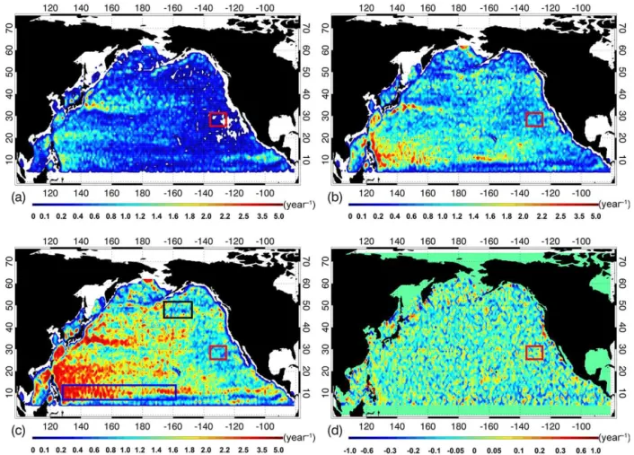
grid. In general, anticyclonic eddies are sig-nificantly more frequent than cyclonic eddies. As shown in Fig. 9a, the cyclonic eddies are mainly located in the west-ern part of the NPO. For example, there are lots of cyclonic eddies east of Japan near the Kuroshio, which can also be seen from both Fig. 1 and the results in Sect. 5.1. In contrast, anticyclonic eddies are mainly located in the eastern part of the NPO (Fig. 9b). For example, the eddies are mainly an-ticyclones in the red box, which can also be seen from the results in Sect. 4.2. In general, the eddies are ubiquitous in Fig. 9c (about 50–70 eddies per year on each 1◦
×1◦
grid), except that there are several regions where both types of ed-dies are relatively scarce. One of them is known as “eddy desert” (black box in Fig. 9c) (Chelton et al., 2007). The other region is the North Equatorial Current (NEC) (blue box in Fig. 9c) (Hu et al., 2015). Finally, we present in Fig. 9d the ratio of the difference of the numbers of cyclonic and anticy-clonic eddies to the total number of eddies.
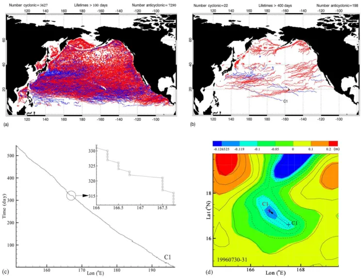
We apply the GEM to these eddies detected by MEI with rc=2/3 andN=2. In the NPO, there are a total of 60 276 eddies with lifetimes longer than 30 days. Among them, 37 553 of the eddies are anticyclonic and 22723 are cyclonic. The tracks of long-lived eddies are plotted in Fig. 10. In general, they are similar to those shown in previous stud-ies (Chelton et al., 2011b). There are 7290 anticyclonic and 3627 cyclonic eddies with lifetimes longer than 100 days (Fig. 10a), and the ratio of anticyclonic to cyclonic eddies is approximately 2. The ratio is larger for eddy lifetimes greater than 400 days, which was also noted in previous stud-ies (Chelton et al., 2011b; Xu et al., 2011). Each track is very smooth because we require that the snapshots of eddies on different days overlap one another. We have done a visual evaluation of many long-lifetime eddy trajectories and the
The SLA field on 30 July 1996 is plotted as contours. The eddy center is marked by a black cross at 167.5◦E, 16.5◦N.
In contrast, the SLA field on 31 July 1996 is plotted in shad-ing. The eddy center is marked by a red cross at 166.75◦E,
17.25◦
N. The distance between the eddy extrema was larger than 100 km within a day. Although that distance is far be-yond the criterion applied in standard eddy tracking routines (Mason et al., 2014; Yi et al., 2015), we can see from the SLA fields that they both indicated the same eddy, and that it was consistent with our approach to connect the trajectories into a single trajectory.
There may be no associated eddy identified at the next time step for an eddy at time stepk, and it may be the result of ed-dies temporarily “disappearing” for a variety of reasons re-lated to sampling errors and measurement noise (Chelton et al., 2011b). The application of our similarity vector and look-ahead procedure can effectively accommodate such problems and allow for the reappearance of a temporarily “disappear-ing” eddy in the tracking procedure. In turn, the application of the similarity vector reduces the usage of the look-ahead procedure. It is clear that the similarity expressed as a vector is better than that as a scalar using simple distance.
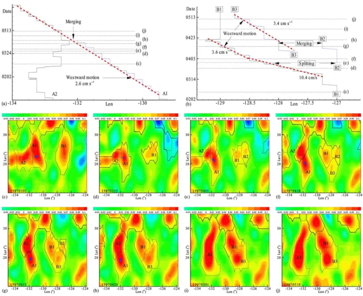
4.2 Eddy merging and splitting
The trajectories provide evidence of dynamic evolution. The time evolution of a couple of anticyclonic eddies is depicted in Fig. 11a, which implies a merging process occurring in the red boxes in Fig. 9. As shown in Fig. 11a, eddy A1 had a westward movement with a speed of 2.6 cm s−1, and eddy A2 lingered near 133◦
W. Then, both eddies merged into one large eddy on 23 April 1997. That evolutionary process is clearly shown by the SLA fields (Fig. 11c–j). In Fig. 11c, there were two anticyclonic eddies, A1 and A2, located at 132◦
W, 28.5◦
N. Eddy A1 moved from east to west with a nearly constant speed of 2.6 cm s−1, whereas eddy A2 had negligible zonal motion. They then rotated clockwise about each other with an average angular velocity of 6×10⁻⁷s−1, as denoted by the blue arrows. Finally, they merged into the new large eddy A2 (see the animation in the Supplement).
Figure 9. (a)The number of cyclonic eddy extrema on each 1◦×1◦grid per year.(b)Same as(a), except for anticyclonic eddies.(c)Same as
(a), except for the total number of eddies.(d)The ratios of the difference in the number of cyclonic and anticyclonic eddies to the total eddies (a logarithmic scale is used). The black box is the “eddy desert”; the blue box is the NEC. The red boxes are the locations of merging/splitting examples in Fig. 11, where anticyclonic eddies dominated.
anticyclonic eddies B1, B2, and B3 are depicted in Fig. 11b. At first, eddy B1 had a fast westward speed of 10.4 cm s−1. It then split into two eddies (B1 and B2) on 29 March 1997 (Fig. 5). Eddy B1 traveled at its original speed, whereas eddy B2 lingered at its origin. Then, eddy B3 emerged at a loca-tion south of B1 and B2 on 9 April 1997, which slowed down the speed of B1 to approximately 3.5 cm s−1. After that, eddy B2 merged into eddy B3 on 19 April 1997. In fact, similar to eddies A1 and A2, eddies B1 and B3 eventually merged into a new eddy on 20 May 1997 (not shown). The SLA maps in Fig. 11c–j show more details that were not recorded by the eddy tracking data. Note that eddy B2 had a very short lifetime of 20 days but a complex dynamic process. If only long-term eddies (lifetime > 30 days) were saved, the corre-sponding evolutionary process might not be recorded prop-erly.
It is expected that a pair of cyclonic eddies will have a counter-clockwise rotation in the Northern Hemisphere, known as the Fujiwhara effect for atmospheric cyclones
(Fu-jiwhara, 1921). When two cyclones are close enough, they will begin to orbit cyclonically (counter-clockwise in the Northern Hemisphere). Because the above-mentioned eddies (A1, A2; B1, B2, B3) are anticyclonic, they have opposing directions of rotation, which appear as two point vortices moving in circular paths about the center of vorticity in clas-sical fluid dynamics (Batchelor, 1967).
4.3 Census of merging and splitting events
To illuminate how often the merging and splitting processes occurred, we counted the total number of merging and split-ting events on each 1◦
×1◦
grid each year. The merging and splitting events were homogeneously distributed in the oceans, but in general were very few times each year per 1◦
×1◦
Figure 10. (a)Tracks of long-lived (> 100 days) eddies.(b)Tracks of long-lived (> 400 days) eddies. In(a)and(b), blue color marks cyclonic eddies, and red color marks anticyclonic eddies.(c)The track of eddy C1. Note the sudden jump from 167.5 to 166.75◦E on 31 July 1996.
(d)The SLA fields on 30 (contours) to 31 July (shading), using the same intervals for the contours and the shadings. The eddy centers are marked by a black cross (30 July) and a red cross (31 July).
Fig. 9a. In contrast, the merging frequency for anticyclonic eddies was larger along the western coast (Fig. 12b), whereas the anticyclonic eddy centers were located mainly in the east (Fig. 9b). Although merging and splitting events may occur anywhere in the ocean, there is spatial variation in the num-ber of events (Fig 12c, d).
The first type of special region is the western boundary. It is known that the western boundary is a sink of eddy energy caused by the interaction with the bottom and lateral topogra-phy (Zhai et al., 2010). It is also known as a “graveyard” for westward-propagating ocean eddies (Zhai et al., 2010; Chel-ton et al., 2011b). The second type of special region is lo-cated in strong currents, including the Kuroshio Current and the NEC (Hu et al., 2015). Among those currents, the eddies in the NEC had the highest frequency of merging and split-ting events, which was not noted in previous studies. The third type of special region is located in the northeastern
Pa-cific, which is also known as an “eddy desert” (Chelton et al., 2007). The fourth type of special region is located in en-closed marginal seas, especially the Bering Sea.
Figure 11.The dynamic evolutions of two groups of eddies, which are located in the red boxes in Fig. 9.(a)Two eddies, A1 and A2, approached each other, and A1 merged with eddy A2, where the blue arrows indicate that the eddy centers rotated clockwise during the merging process.(b)In the meantime, eddy B1 split into two small eddies.(c–j)The evolutions of SLA fields and eddies. Note that eddies A1 and A2 had clockwise rotations when they approached each other, as indicated by the blue arrows in(c)–(h).
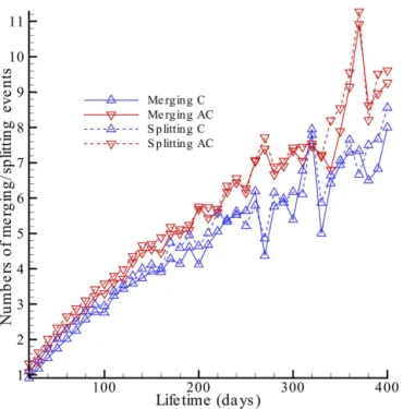
We also calculate the average dynamic (merging and split-ting) events per eddy as a function of lifetime (Fig. 13). The results are similar regardless of eddy polarizations and dy-namic types. The merging and splitting events increase ap-proximately linearly with eddy lifetime. However, merging and splitting events are more frequent for anticyclonic eddies than for cyclonic eddies.
5 Discussion 5.1 Data noise
Although AVISO product DT1 is much better than previous products, there are still some notable errors, especially for short temporal scales of less than 2 months (Carrere et al.,
2016). It was reported that there are along-track SLA errors of about 2–3 cm globally and of more than 3 cm at high lati-tudes and in shallow waters.
To reduce the noise in SLA data, one may use the Gaus-sian structure filter (Chelton et al., 2011b; Mason et al., 2014), Hanning filters (Penven et al., 2005), or Lanczos fil-ters (Chaigneau et al., 2008). As certain paramefil-ters need to be chosen in these filters, the filtered results depend much on these parameters (see Fig. A1 in Chelton et al., 2011b). As a sensitivity test we apply a simple five-point quadratic smoothing to the SLA data. The filtered data are then piece-wise C2-smoothed by a quadratic function, which satisfies the potential requirements for calculating vorticity (second derivative of SLA) from SLA data.
Figure 12.The frequencies of dynamic processes per 1◦×1◦grid element.(a)The merging frequency for cyclonic eddies.(b)The merging frequency for anticyclonic eddies.(c)The merging frequency for all eddies.(d)The ratios of the difference between the frequencies of merging and splitting for all eddies to the sum of merging and splitting frequencies for all eddies. The boxes are the same as in Fig. 9. The blue box is the location of NEC, where the merging frequency is high.
are very close to the non-smoothed SLA maps and the values at the SLA extrema (not shown) are close to their original values. This implies that the noise in the DT14 data is suffi-ciently small for our purpose.
However, the noise cannot be neglected, even when it is small. It might induce additional SLA extrema (see the def-inition of an extremum in Sect. 2.2), which eventually af-fect eddy detection, e.g., the additional extremum on 2 uary 1993 in box A and the additional extremum on 3 Jan-uary 1993 in box B (Fig. 14). These additional extrema ex-isted only for a very short period (1 or 2 days), but they can induce additional merging and splitting events, which may cause eddies to unexpectedly terminate (Chelton et al., 2011b). The ambiguity of the eddy identification procedure, which may be caused by sampling errors and measurement noise in the input SLA data, strongly suggests the application of a look-ahead approach.
5.2 Impact of variations of parameters
To discuss the impact of the GEM critical valuercand look-ahead timeN, we carry out a sensitivity study in the North Pacific from year 1993 to 2012. The number of eddies with lifetimes > 30 days is counted for different rc and N, as shown in Fig. 15a. Note that the results are very similar, ex-cept forN=0 (i.e., without any look-ahead). It is from the
above discussion that we see look-ahead is necessary when there are extrema due to small noise in the data. The number of eddies does not change substantially withrcfor anyN> 1, whenrcis within 0.5 to 0.8 (e.g., 63 469 eddies were iden-tified withN=2,rc=0.5, and the identified eddy number was 63 630 withN =4,rc=0.8). Meanwhile, the numbers of merging and splitting events (lifetimes > 30 days) are also counted for differentrcandN, as shown in Fig. 15b. In gen-eral, the splitting events occur slightly more frequently than the merging events (e.g., 122 876 splitting events and 122382 merging events forN=2,rc=0.5). Note also that the results are very similar, except forN=0. The numbers of merging
in-Figure 13. The number of merging/splitting events per eddy as a function of eddy lifetime, where AC and C represent anticyclonic and cyclonic eddies.
creases. For eachN> 0, the numbers of merging and splitting events reach a maximum atrc =0.6. A relatively loose sim-ilarity condition (rc< 0.5) will lead to a risk of eddy jumping from one track to another, which consequently reduces both total eddy number and dynamic events. On the other hand, a relatively strict similarity condition (rc> 0.9) will lead to a risk of missing eddies, which may also reduce both total eddy numbers and dynamic events.
In general, one would like the tracking results to be insen-sitive to the choice of these parameters. From Fig. 15, we can observe that 0.5 <rc< 0.8 appears to be a choice with relatively robust results. The optimal value for rc might be 0.6–0.7, which is reasonable. On the one hand, we first re-quire that rc> 0.5. On the other hand, we know there is er-ror (∼10 %) in calculating eddy area since only eddy grids
are taken into consideration. This is also the reason why we need rc< 0.9 or even smaller. So the optimal value should be within 0.5–0.9, and∼0.7 is just in this middle. We also find that the look-ahead time N should be larger than 0; otherwise, the risks of eddy jumping and eddy missing are too great. The look-ahead approach effectively reduces such risks. For example,N=1 andN=2 have, respectively, 95.5 and 98 % of the total eddies forN=4. To reduce the missing eddies to 1 %, the look-ahead time might be greater than 6 days. This is also the physical requirement of the representa-tive period of the merged SLA data (Chelton et al., 2011b). AlthoughN=4 might be better,N=2 produced a very
sim-ilar result (∼2 % bias to N=4) and with a significantly
Table 1.The census of long-lived eddies, where “Amp” represents the amplitude threshold used in eddy detection, and “C” and “AC”, respectively, represent cyclonic and anticyclonic eddies.
Amp AC C AC C
(> 100 days) (> 100 days) (> 400 days) (> 400 days)
1 cm 7290 3627 198 22
3 cm 7118 3550 194 21
lower computational cost. Our present parameters are rea-sonable considering the computational cost.
It should be pointed out that the GEM is relatively inde-pendent of MEI, but the ratiosr1,r2, andrcmight be sensi-tive to the method used in eddy identification. We noted that the GEM based on Okubo–Weiss (O–W) parameter identi-fication is more sensitive to the critical valuerc than is the SLA-based GEM, since O–W-based eddies are much smaller and more possibly unreal (Chaigneau et al., 2008). Besides, rc may not be independent ofN, and the presentrc should only be valid for small time steps. If the time step is too large, eddies may move too far so that eddy snapshots can-not overlap with each other. This constraint for time step is something like the Courant–Friedrichs–Lewy (CFL) condi-tion (for time step) in computer fluid dynamics. In general, we think any tracking method should have this time-step lim-itation (depending on eddy size/propagation speed), if one does not want to mix one signal with another.
Finally, as noted in Sect. 4.2, there are short-term eddies (lifetime < 30 days), which might experience complex evolu-tion processes. If only long-term eddies (lifetime > 30 days) were saved, the corresponding evolution process might not be recorded properly. This should be noted in further appli-cations on eddy dynamics with satellite altimetry data. 5.3 Impact of the eddy boundary
Different identification methods may give different eddy boundaries, although the eddy center is relatively robust. Eddy area S is sensitive to the eddy boundary, but it is diffi-cult to compare directly the influence of eddy boundary dif-ferences that result from the identification method choice. However, the area ratio reduces the sensitivity to the eddy area S because both the overlap area S12 and the eddy area S change synchronously. Moreover, our tracking results for-tunately are not very sensitive torc (or the eddy area S), as noted in the above discussion. For example, the present re-sults are based on a very strict identification method. If we modify the threshold of eddy amplitude from 1 to 3 cm, the number of identified eddies will decline. Nevertheless, the identification results for the long-lived eddies appear to be similar (Table 1).
Figure 14.Comparison of the non-smoothed(a)and smoothed SLA data(b)from 1 to 4 January 1993, where the color field shows SLA, white dots mark eddy centers, and two boxes A and B mark the regions sensitive to noise. Note that small noise affected the eddy detection.
comparison of eddies identified by different methods, since the eddy detection algorithms differ a lot from each other. In general, the automated eddy detection algorithms are cat-egorized into three types: (1) physical parameter-based al-gorithms, e.g., the Okubo–Weiss (O–W) parameter (Isern-Fontanet et al., 2003; Chaigneau et al., 2008); (2) flow geometry-based algorithms (Chaigneau et al., 2011; Chelton et al., 2011b; Wang et al., 2015); and (3) hybrid methods,
Figure 15. (a)Number of eddies (lifetime > 30 days) vs. the critical valuercand look-ahead timeN.(b)Number of merging and splitting events (lifetime > 30 days) vs. the critical valuercand look-ahead timeN.
5.4 Future research
The GEM is a flexible model that can easily work with other relevant programs, e.g., data filtering and smoothing algo-rithms (Chelton et al., 2011b; Ienna et al., 2014; Wang et al., 2014), other hybrid eddy detection algorithms (e.g., Yi et al., 2015), and O–W parameter detection (e.g., Petersen et al., 2013), because the GEM only requires a flow field and pre-viously identified eddies to accomplish dynamic tracking. In addition, the similarity measurement can be replaced by sim-ilar methods (e.g., Pegliasco et al., 2015) when considering more complex conditions.
Eddies identified by using algorithms without watershed segmentation can also be tracked with the GEM. In this case, the strong interaction stage of eddies “in conjunction”, which leads to genesis and termination of eddies, is more likely missed, as pointed out in Sect. 2.3. However, the weak in-teraction stage of eddies (watershed free) in some far dis-tance could still be recorded, because most merging/splitting records occurred at the interaction of two eddies with a cer-tain distance. This weak interaction still cannot be recorded by a previously interaction-free tracking algorithm, which records only the isolated tracks. Thus the GEM extends the potential applications of previously identified eddies.
The GEM is a complex model. The output data include eddy tracks, relationships, and previously identified eddy characteristics (e.g., amplitude and radius). These eddy char-acteristics, which were directly obtained from the identifica-tion process, are useful for censuses (Chelton et al., 2011b). However, they may not be sufficiently accurate for some ap-plications. For example, eddy area was required in our recent studies on typhoons and oceanic eddy interactions (Sun et al., 2010, 2012, 2014). Besides, some physical quantities
(circu-lation, angular momentum, energy) are required to be accu-rately calculated in the investigation of eddy dynamics pro-cess. A better way to obtain these characteristics might be to use a nonlinear fitting of the flow field (Wang et al., 2015; Yi et al., 2015) with appropriate models (e.g., Sun, 2011; Zhang et al., 2013) rather than simply estimation from identifica-tion.
Another future research direction may involve comparing different tracking datasets. Because there are several tracking datasets produced by various methods, it is useful to inter-compare them. This may improve both the tracking methods and the available datasets for further studies.
The GEM can be easily applied to larger datasets, even to 3-D numerical simulation outputs (Petersen et al., 2013; Woodring et al., 2016), because its computational time in-creases only linearly as a function of the size of the dataset. The computation of the 20-year daily global SLA data only required a few hours on a personal computer. In a personal computer with a CPU of i7-6700 k and 4.00 GHz, it takes about 15 min to identify snapshots of eddies, about 20 min to establish similarity, and about 10 min to track eddies in the North Pacific Ocean (NPO) with 0.25◦×
0.25◦
resolution of 20-year daily “DT14” data. Such a model can be used to an-alyze numerical simulation outputs.
identi-complexity is ofO(LM(N+1)T ). We applied the GEM to the eddies in the North Pacific. Eddy tracks were smooth because we required that the snapshots of eddies on neigh-boring days overlap one another. Both merging and splitting rates of eddies were high, especially at the western bound-ary and in strong currents. The GEM is useful not only for satellite-based observational data, but also for the output of numerical simulations. It potentially has many applications for studies of dynamic processes in related fields, e.g., the dynamics of cyclones in meteorology. The MEI and GEM computer codes and program manual will be provided openly (see the model code in the Supplement) and at the web-site https://www.researchgate.net/profile/Liang_Sun20/ after publication of this paper.
The Supplement related to this article is available online at doi:10.5194/os-12-1249-2016-supplement.
Acknowledgements. We thank the anonymous referees and John M. Huthnance for their comments and sugges-tions. We thank the AVISO for providing the SLA data (http://www.aviso.oceanobs.com/). This work was supported by the National Basic Research Program of China (nos. 2012CB417402 and 2013CB430303), National Programme on Global Change and Air-Sea Interaction (GASI-IPOVAI-04), the National Foundation of Natural Science of China (no. 41376017) and the Open Fund of the State Key Laboratory of Satellite Ocean Environment Dynamics (no. SOED1501).
Edited by: J. M. Huthnance
Reviewed by: J. M. Huthnance and three anonymous referees
References
Batchelor, G. K.: An introduction to fluid dynamics, Cambridge university press, 615 pp., 2000.
Bennett, A. F. and White, W. B.: Eddy heat flux in the subtropical North Pacific, J. Phys. Oceanogr., 16, 728–740, 1986.
Argo profiling floats, J. Geophys. Res.-Oceans, 116, C11025, doi:10.1029/2011JC007134, 2011.
Chelton, D. B. and Schlax, M. G.: Global observations of oceanic Rossby waves, Science, 272, 234–238, 1996.
Chelton, D. B., Schlax, M. G., Samelson, R. M., and de Szoeke, R. A.: Global observations of large oceanic eddies, Geophys. Res. Lett., 34, L15606, doi:10.1029/2007GL030812, 2007.
Chelton, D. B., Gaube, P., Schlax, M. G., Early, J. J., and Samel-son, R. M.: The influence of nonlinear mesoscale eddies on near-surface oceanic chlorophyll, Science, 334, 328–332, 2011a. Chelton, D. B., Schlax, M. G., and Samelson, R. M.: Global
ob-servations of nonlinear mesoscale eddies, Progr. Oceanogr, 91, 167–216, 2011b.
Dong, C., Nencioli, F., Liu, Y., and McWilliams, J. C.: An auto-mated approach to detect oceanic eddies from satellite remotely sensed sea surface temperature data, IEEE Geosci. Remote Sens. Lett., 8, 1055–1059, 2011.
Dong, C., McWilliams, J. C., Liu, Y., and Chen, D.: Global heat and salt transports by eddy movement, Nat. Commun., 5, 3294, doi:10.1038/ncomms4294, 2014. Duacs/AVISO: A new version of SSALTO/Duacs products available in April 2014, Version 1.1, CNES, available at: http://www.aviso.altimetry.fr/fileadmin/ documents/data/duacs/, 2014.
Fang, F. and Morrow, R.: Evolution, movement and decay of warm-core Leeuwin Current eddies, Deep-Sea Res. Pt. II, 50, 2245– 2261, 2003.
Fujiwhara, S.: The natural tendency towards symmetry of motion and its application as a principle in meteorology, Q. J. Roy. Me-teor. Soc., 47, 287–293, doi:10.1002/qj.49704720010, 1921. Faghmous, J. H., Uluyol, M., Styles, L., Le, M., Mithal, V., Boriah,
S., and Kumar, V.: Multiple Hypothesis Object Tracking For Un-supervised Self-Learning: An Ocean Eddy Tracking Application, in: AAAI, 2013.
Hu, D., Wu, L., Cai, W., Gupta, A. S., Ganachaud, A., Qiu, B., and Wang, G.: Pacific western boundary currents and their roles in climate, Nature, 522, 299–308, 2015.
Ienna, F., Jo, Y. H., and Yan, X. H.: A new method for tracking Meddies by satellite altimetry, J. Atmos. Ocean. Technol., 31, 1434–1445, 2014.
Li, Q. Y. and Sun, L.: Technical Note: Watershed strategy for oceanic mesoscale eddy splitting, Ocean Sci., 11, 269–273, doi:10.5194/os-11-269-2015, 2015.
Li, Q. Y., Sun, L., Liu, S. S., Xian, T., and Yan, Y. F.: A new mononuclear eddy identification method with simple splitting strategies, Remote Sens. Lett., 5, 65–72, doi:10.1080/2150704X.2013.872814, 2014.
Mason, E., Pascual, A., and McWilliams, J. C.: A new sea surface height–based code for oceanic mesoscale eddy tracking, J. At-mos. Ocean. Technol., 31, 1181–1188, 2014.
McGillicuddy, D. J.: Eddies masquerade as planetary waves, Sci-ence, 334, 318–319, doi:10.1126/science.1208892, 2011. Nencioli, F., Dong, C., Dickey, T., Washburn, L., and McWilliams,
J. C.: A vector geometry-based eddy detection algorithm and its application to a high-resolution numerical model product and high-frequency radar surface velocities in the Southern Califor-nia Bight, J. Atmos. Ocean. Technol., 27, 564–579, 2010. Pegliasco, C., Chaigneau, A., and Morrow, R.: Main eddy
ver-tical structures observed in the four major Eastern Boundary Upwelling Systems, J. Geophys. Res.-Oceans, 120, 6008–6033, doi:10.1002/2015JC010950, 2015.
Penven, P., Echevin, V., Pasapera, J., Colas, F., and Tam, J.: Average circulation, seasonal cycle, and mesoscale dynamics of the Peru Current System: A modeling approach, J. Geophys. Res., 110, C10021, doi:10.1029/2005jc002945, 2005.
Petersen, M. R., Williams, S. J., Maltrud, M. E., Hecht, M. W., and Hamann, B.: A three-dimensional eddy census of a high-resolution global ocean simulation, J. Geophys. Res.-Oceans, 118, 1759–1774, 2013.
Sun, L.: A typhoon-like vortex solution of incompressible 3D inviscid flow, Theor. Appl. Mech. Lett., 1, 042003, doi:10.1063/2.1104203, 2011.
Sun, L., Yang, Y.-J., Xian, T., Lu, Z., and Fu, Y.-F.: Strong enhance-ment of chlorophyll a concentration by a weak typhoon, Mar. Ecol. Prog. Ser., 404, 39–50, doi:10.3354/meps08477, 2010. Sun, L., Yang, Y.-J., Xian, T., Wang, Y., and Fu, Y.-F.: Ocean
re-sponses to Typhoon Namtheun explored with Argo floats and multiplatform satellites, Atmos. Ocean., 50, 15–26, 2012.
Sun, L., Li, Y.-X., Yang, Y.-J., Wu, Q., Chen, X.-T., Li, Q.-Y., Li, Y.-B., and Xian, T.: Effects of super typhoons on cyclonic ocean eddies in the western North Pacific: A satellite data-based eval-uation between 2000 and 2008, J. Geophys. Res.-Oceans, 119, 5585–5598, doi:10.1002/2013JC009575, 2014.
Wang, R., Yang, Z., Liu, L., Deng, J., and Chen, F.: Decoupling noise and features via weighted L1-analysis compressed sensing, ACM Transactions on Graphics (TOG), 33, 1–12, 2014. Wang, Z., Li, Q., Sun, L., Li, S., Yang, Y., and Liu, S.: The
most typical shape of oceanic mesoscale eddies from global satellite sea level observations, Front. Earth Sci., 9, 202–208, doi:10.1007/s11707-014-0478-z, 2015.
Woodring, J., Petersen, M., Schmeiber, A., Patchett, J., Ahrens, J., and Hagen, H.: In Situ Eddy Analysis in a High-Resolution Ocean Climate Model, IEEE Trans. Visual. Comput. Graph., 22, 857–866, doi:10.1109/TVCG.2015.2467411, 2016.
Xiu, P., Chai, F., Shi, L., Xue, H., and Chao, Y.: A census of eddy activities in the South China Sea during 1993–2007, J. Geophys. Res.-Oceans, 115, C03012, doi:10.1029/2009JC005657, 2010. Xu, C., Shang, X. D., and Huang, R. X.: Estimate of eddy
en-ergy generation/dissipation rate in the world ocean from altime-try data, Ocean Dynam., 61, 525–541, 2011.
Yang, G., Wang, F., Li, Y., and Lin, P.: Mesoscale eddies in the northwestern subtropical Pacific Ocean: Statistical characteris-tics and three-dimensional structures, J. Geophys. Res.-Oceans, 118, 1906–1923, 2013.
Yi, J., Du, Y., Zhou, C., Liang, F., and Yuan, M.: Automatic Identifi-cation of Oceanic Multieddy Structures From Satellite Altimeter Datasets, IEEE JSTARS, 8, 1555–1563, 2015.
Zhai, X., Johnson, H. L., and Marshall, D. P.: Significant sink of ocean-eddy energy near western boundaries, Nat. Geosci., 3, 608–612, 2010.
Zhang, C. H., Xi, X. L., Liu, S. T., Shao, L. J., and Hu, X. H.: A mesoscale eddy detection method of specific intensity and scale from SSH image in the South China Sea and the North-west Pacific, Science China: Earth Sciences, 57, 1897–1906, doi:10.1007/s11430-014-4839-y, 2014.