An isopycnic ocean carbon cycle model

(1)

GMDD

2, 1023–1079, 2009

Isopycnic ocean carbon cycle model

K. Assmann et al.

Title Page

Abstract Introduction

Conclusions References

Tables Figures

◭ ◮

Back Close

Full Screen / Esc

Printer-friendly Version

Interactive Discussion

Geosci. Model Dev. Discuss., 2, 1023–1079, 2009 www.geosci-model-dev-discuss.net/2/1023/2009/ © Author(s) 2009. This work is distributed under the Creative Commons Attribution 3.0 License.

Geoscientific Model Development Discussions

Geoscientific Model Development Discussionsis the access reviewed

discussion forum ofGeoscientific Model Development

An isopycnic ocean carbon cycle model

K. M. Assmann1,2, M. Bentsen1,3, J. Segschneider4, and C. Heinze1,2

1

Bjerknes Centre for Climate Research, Bergen, Norway

2

Geophysical Institute, University of Bergen, Bergen, Norway

3

Nansen Remote Sensing and Environmental Research Centre, Bergen, Norway

4

Max-Planck Institute for Meteorology, Hamburg, Germany

Received: 1 July 2009 – Accepted: 3 July 2009 – Published: 27 July 2009 Correspondence to: K. M. Assmann (karen.assmann@bjerknes.uib.no)

(2)

GMDD

2, 1023–1079, 2009

K. Assmann et al.

Title Page

Tables Figures

◭ ◮

Back Close

Full Screen / Esc

Abstract

The carbon cycle is a major forcing component in the global climate system. Modelling studies aiming to explain recent and past climatic changes and to project future ones thus increasingly include the interaction between the physical and biogeochemical sys-tems. Their ocean components are generallyz-coordinate models that are

conceptu-5

ally easy to use but that employ a vertical coordinate that is alien to the real ocean structure. Here we present first results from a newly developed isopycnic carbon cycle model and demonstrate the viability of using an isopycnic physical component for this purpose. As expected, the model represents interior ocean transport of biogeochem-ical tracers well and produces realistic tracer distributions. Diffi_{culties in employing a}

10

purely isopycnic coordinate lie mainly in the treatment of the surface boundary layer which is often represented by a bulk mixed layer. The most significant adjustments of the biogeochemical code for use with an isopycnic coordinate are in the representa-tion of upper ocean biological producrepresenta-tion. We present a series of sensitivity studies exploring the eff_{ect of changes in biogeochemical and physical processes on export}

15

production and nutrient distribution. Apart from giving us pointers for further model development, they highlight the importance of preformed nutrient distributions in the Southern Ocean for global nutrient distributions. Use of a prognostic slab atmosphere allows us to assess the eff_{ect of the changes in export production on global ocean}

car-bon uptake and atmospheric CO₂levels. Sensitivity studies show that iron limitation for

20

(3)

GMDD

2, 1023–1079, 2009

K. Assmann et al.

Title Page

Tables Figures

◭ ◮

Back Close

Full Screen / Esc

1 Introduction

The human induced increase of atmospheric greenhouse gases, especially that of CO₂, has led to growing concern about the climatic and environmental consequences related to these perturbations. The ocean plays an important role in the regulation of atmospheric gases (e.g., Sillen, 1966). It is known as to represent the major ultimate

5

sink for anthropogenic CO₂ (e.g., Bolin and Eriksson, 1957; Archer, 2005) due to its relatively quick turnover time scale of 1000–2000 years (Matsumoto et al., 2007) and its high buff_{er capacity for CO}

2additions (Buch et al., 1932; Revelle and Suess, 1957). For

correct predictions of the development of the Earth’s carbon budget during the coming decades and centuries under given greenhouse gas emission scenarios, the kinetics

10

of marine CO₂ uptake from the atmosphere play a crucial role: how quickly can the ocean neutralise CO₂additions to the atmosphere through input from fossil fuel burning and cement manufacturing (Boden et al., 2009) as well as land use (Houghton, 1999)? Further, in recent years, carbon cycle climate feedbacks have been identified to provide a major uncertainty in future projections of climate change (Denman et al., 2007). It is

15

likely that these feedbacks will reinforce climate change, but feedback strength varies considerably among diff_{erent model systems (Friedlingstein et al., 2006).}

While quantifying the regulation of the Earth’s radiative budget is a key question, we require coupled physical-biogeochemical ocean models to address a number of additional important issues. The rising carbon content of the ocean causes a drop in

20

pH (ocean acidification) with potentially severe impacts for marine biota and related geochemical cycles (Caldeira and Wickett, 2003; Raven et al., 2005). The pH changes have to be predicted appropriately with respect to space and time and impacts such as metal speciation on biogeochemical cycling have to be quantified and upscaled to the Earth system. Global nutrient cycling is undergoing significant changes (Duce et al.,

25

(4)

GMDD

2, 1023–1079, 2009

K. Assmann et al.

Title Page

Tables Figures

◭ ◮

Back Close

Full Screen / Esc

of poorly ventilated water masses in the oceans and sinking oxygen water column levels on the large scale (e.g., Whitney et al., 2007; Oschlies et al., 2008).

In addition to these pressing questions, major fundamental oceanographic questions are still not answered conclusively and need model tools for clarification. We are as yet not able to explain the glacial-interglacial variations in atmospheric CO₂concentration

5

(Archer et al., 2000; Sigman and Boyle, 2000; Toggweiler et al., 2006) for which the ocean has to play a major role. Marine particle fluxes, which provide the major link between the input of matter to the oceans from aeolian deposition as well as river loads and the output of matter through sedimentation and reverse weathering, are not yet well quantified due the diffi_{culties in measuring biological export production rates}

10

and particle fluxes through the water column (e.g., Iverson et al., 2000; Buesseler et al., 2007). The marine paleoclimatic record, which is the result of a complex chain of transfer functions which map environmental and climatic change onto the marine sediment, needs explanation and exploitation for the calibration of climate models. In addition, the fate of toxic or otherwise hazardous substances in the oceans has to

15

be identified and quantified including the realistic transport of CO₂ from leaks out of purposefully established sub-sea carbon storage reservoirs (IPCC, 2005).

So far, only a relatively small number of global interactive carbon cycle climate mod-els (“Earth system modmod-els”, to be extended also with respect to other processes and cycles) exist. The ocean components in these systems for ocean physics (velocity field,

20

density field, and sea ice) as well as biogeochemistry (inorganic chemsitry, biological particle production and degradation, input and output of matter) are conceptually rela-tively closely related. The ocean biogeochemical models are either inorganic models (without a representation of the marine biosphere, e.g., Maier-Reimer and Hassel-mann, 1987), “particles only models” representing only biological export production

25

(based on phytoplankton production, e.g., Bacastow and Maier-Reimer, 1990; Najjar et al., 1992), or diff_{ering numbers functional groups and zooplankton (NPZD models}

(5)

GMDD

2, 1023–1079, 2009

K. Assmann et al.

Title Page

Tables Figures

◭ ◮

Back Close

Full Screen / Esc

further include an interactive sediment (Archer and Maier-Reimer, 1994; Heinze et al., 1999; Maier-Reimer et al., 2005; Ridgwell and Hargreaves, 2007; Gehlen et al., 2008). Due to the lack of suffi_{cient knowledge of the “first principles” governing life processes}

in the ocean, biogeochemical ocean modelling is still in its developmental phase. The various physical ocean models are mostly based on the Primitive Equations (full

5

set of temporally averaged Navier-Stokes equations), usually discretised on a C-grid (Arakawa and Lamb, 1977) within az-coordinate framework, i.e., the water column is discretised vertically with respect to fixed depth intervals. For physical tracer transport in the ocean, it is intriguing to explore alternative formulations, since diff_erent

mod-els still diff_{er significantly with respect to reproducing global tracer distributions (Doney}

10

et al., 2004; Orr, 2002). While permitting an accurate computation of the horizontal pressure gradient driving geostrophic flow, vertical discretization onz-levels leads to spurious diapycnal mixing and upwelling. Even though the widely used parameterisa-tion of ocean mixing due to large-scale turbulence after Gent and McWilliams (1990) has been shown to be a suitable formulation for oceanic mixing in ocean models,

isopy-15

cnic ocean models have an advantage over those with geometric vertical layers. Their vertical coordinate mimics the real structure of the water column as stratified layers of constant density, and thus avoids artificial mixing and advection in the ocean interior. Their disadvantages include the problem of massless layers, the necessity of adding a mixed layer model to adequately represent surface processes, and the induction of a

20

horizontal pressure gradient error by the sloping density surfaces. Models with diff

er-ent vertical schemes thus complemer-ent each other and can be used as one basis for an uncertainty assessment.

We present here a new coupled isopycnic physical-biogeochemical model based on two already well established components: the dynamical isopycnic ocean model

25

(6)

GMDD

2, 1023–1079, 2009

K. Assmann et al.

Title Page

Tables Figures

◭ ◮

Back Close

Full Screen / Esc

(Matsumoto et al., 2004), integrations including nutrients, oxygen, and carbon had to be limited to short periods since the computations were too demanding for resources at the time (Drange, 1996).

Initially, we will give a description of the model components and the changes made to HAMOCC to make it compatible with an isopycnic ocean model. After this we

eval-5

uate the circulation and temperature and salinity distributions in the physical model. We evaluate the main biogeochemical model parameters with respect to the physical results and present results from several sensitivity studies. In addition, we will also consider the uptake of anthropogenic CO₂ in the model and discuss the conclusions that can be drawn from a stand-alone ocean carbon cycle model with a prognostic slab

10

atmosphere.

2 Model Description

2.1 The physical ocean model MICOM

The numerical methods and thermodynamics of MICOM are documented in Bleck and Smith (1990), and Bleck et al. (1992). Several important aspects deviate from the

15

original model in the version of MICOM used in this study. Since the model version employed here includes several new features that have not been published, we will give a fairly detailed model description and evaluate model performance on a global scale, with a particular view on the influence of the physical model on biogeochemistry. We use incremental remapping as an advection algorithm as proposed by Dukowicz

20

and Baumgardner (2000). This multi-dimensional, second order accurate algorithm is expressed in flux form and assures conservation for tracers. It also guarantees mono-tonicity for tracers for any velocity field that does not violate the Courant-Friedrichs-Levy condition of the method. Neither of these conditions was assured in the origi-nal flux-corrected transport (FCT) scheme (Zalesak, 1979), used for layer thickness

25

(7)

GMDD

2, 1023–1079, 2009

K. Assmann et al.

Title Page

Tables Figures

◭ ◮

Back Close

Full Screen / Esc

MICOM. While the incremental remapping is computationally rather expensive for one tracer, the cost of adding additional tracers and age tracers is modest which makes it well-suited for use with a ocean carbon cycle module that contains a large number of passive tracers.

The original MICOM uses potential density, ρr, with reference pressure at 0 db as 5

the vertical coordinate. This ensures that the very diff_{erent flow and mixing}

character-istics in neutral and dia-neutral directions is well represented near the surface since isopycnals and neutral surfaces are similar near the reference pressure. For pressures that diff_{er substantially from the reference pressure, this does not hold. In this study, we}

choose a reference pressure of 2000 db as the non-neutrality of the isopycnals in the

10

world ocean is then reduced compared to having the reference pressure at the surface (McDougall and Jackett, 2005).

2.1.1 Pressure gradient force

Traditionally, MICOM expresses the pressure gradient force (PGF) as a gradient of a potential on an isopycnic surface,

15

1

ρ∇zp≈ ∇ρrM, (1)

as such a formulation has favourable numerical properties (Hsu and Arakawa, 1990). This is only accurate if the density can be considered as a function of potential density and pressure alone. This is not the case (de Szoeke, 2000) and assuming such a functional form of density causes large PGF errors when the pressure is substantially

20

diff_{erent from the reference pressure. There have been several attempts to modify}

the MICOM PGF formulation (1) in order to incorporate the eff_{ects of a more}

accu-rate representation of density (Sun et al., 1999; Hallberg, 2005). Inspired by recent work of Rainer Bleck (personal communication, 2006), we have based our formulation on Janji´c (1977) where the PGF is expressed as a gradient of the geopotential on a

(8)

GMDD

2, 1023–1079, 2009

K. Assmann et al.

Title Page

Tables Figures

◭ ◮

Back Close

Full Screen / Esc

pressure surface

1

ρ∇zp=∇pφ. (2)

The geopotential at a certain pressurepis found by integrating the hydrostatic equation from the invariant geopotential at the bottom,φb:

φ=_φ_b₋

Zp

p_b

d p

ρ . (3)

5

A suitable functional form of the equation of state has been chosen, inspired by Jack-ett et al. (2005), that ensures an accurate representation of density compared to the Feistel (2004) equation of state and an analytic expression for the integral in Eq. (3).

2.1.2 Diapycnal mixing

The diff_{usivity of diapycnal turbulent mixing,} _ν

d, in the model is the sum of a back-10

ground diff_{usivity and a Richardson number dependent di}ff_usivity:

νd =νb+νr, (4)

ν_b= C

N, νr =ν0max 





0,1− Rig

Ri₀

!2



 3

, (5)

N2= g

ρ ∂ρ

∂z, Rig =

N2

(∂u/∂z)2+₍_∂v/∂z₎2, (6)

15

(9)

GMDD

2, 1023–1079, 2009

K. Assmann et al.

Title Page

Tables Figures

◭ ◮

Back Close

Full Screen / Esc

10−7 m2s−2, while the critical Richardson number is Ri₀ =_{1. The maximum} _Ri

g

de-pendent diff_usivity_ν

0is set to 500×10− 4

m2s−1in the 300 m closest to the ocean floor to parameterize gravity current mixing, and 50×10−4m2s−1elsewhere to parameterize shear instability mixing. The numerical implementation of the diapycnal mixing follows the scheme of McDougall and Jackett (2005) but with additional care in handling the

5

vigorous mixing due to shear instabilities. The original MICOM only used the back-ground diff_{usivity, and the addition of the}_Ri

gdependent diffusivity greatly improves the

water mass characteristics downstream of overflow regions.

2.1.3 Lateral turbulent mixing

Lateral turbulent mixing of momentum and tracers is parameterized by Laplacian

dif-10

fusion where diff_{usive velocities (di}ff_{usivities divided by the local grid size} ∆_{) of}

mo-mentum and tracers are 1.0×10−2m s−1 and 0.35×10−2m s−1, respectively. With a grid size of about 130 km at 60◦N and 60◦S this gives actual minimum diff_usivities

of 1300 m2s−1 and 455 m2s−1 for momentum and tracers, respectively. Layer in-terfaces are smoothed with biharmonic diff_{usion with a di}ff_{usive velocity (biharmonic}

15

diff_{usivity divided by} ∆3_{) of 1}_.₀_×₁₀−2 _{m s}−1 _{giving a minimum di}ff_{usivity of about}

2.2×1013m4s−1.

2.1.4 Sea-ice

The thermodynamic module incorporates freezing and melting of sea-ice and snow covered sea-ice (Drange and Simonsen, 1996) and is based on the

thermodynam-20

ics of Semtner (1976). The dynamic part of the sea-ice module follows the viscous-plastic rheology of Hibler (1979). The dynamic ice module has been further modified by Harder (1996) to include description of sea-ice roughness and the age of sea-ice. A third order weighted essential non-oscillatory scheme (Liu et al., 1994) is used for the advection of sea-ice fraction, thickness, and age.

(10)

GMDD

2, 1023–1079, 2009

K. Assmann et al.

Title Page

Tables Figures

◭ ◮

Back Close

Full Screen / Esc

2.2 The ocean carbon cycle model HAMOCC 5.1

A detailed description of HAMOCC 5.1 is given in Maier-Reimer et al. (2005). The model is based on the work by Maier-Reimer (1993) and has been used to analyse contemporary ocean carbon fluxes coupled to the physical ocean model MPIOM (Mars-land et al. 2003) in Wetzel et al. (2005). Here we only summarise its main features

5

and those that deviate from this description either because they were introduced later or because they bear on the inclusion of HAMOCC in an isopycnic ocean model. The values of key parameters are summarised in Table 1.

HAMOCC5.1 model uses the formulation of inorganic carbon chemistry in following Maier-Reimer and Hasselmann (1987). Surface pCO₂ is computed as a function of

10

prognostic alkalinity, total DIC, temperature, pressure, and salinity. Dissolution of cal-cium carbonate at depth is a function of carbonate ion saturation state and a constant dissolution rate. The air-sea gas exchange processes of CO₂, oxygen and nitrogen are a function of gas solubility, transfer velocity, and the diff_{erence between partial}

pressure tracers in air and water following Wanninkhof (1992). The model uses gas

15

tracer solubilities according to Weiss (1970) and Weiss (1974), whereas the gas trans-fer velocity depends on the Schmidt number and prognostic wind speed at the surface. HAMOCC5.1 contains a simple diff_{usive slab atmosphere which allows the prognostic}

computation of atmospheric CO₂ levels for a stand-alone ocean set-up of the model forced by atmospheric reanalyses.

20

The model includes an ecosystem model of the NPZD (Nutrient-Phytoplankton-Zooplankton-Detritus) class (Six and Maier-Reimer, 1996) with nutrient co-limitations by phosphate, nitrate and iron (Aumont et al., 2003). Nutrient, carbon, and oxygen uptake and re-dissolution are treated according to Redfield stoichiometry. Growth of the single phytoplankton class is described by Michaelis-Menten kinetics and is in

ad-25

(11)

GMDD

2, 1023–1079, 2009

K. Assmann et al.

Title Page

Tables Figures

◭ ◮

Back Close

Full Screen / Esc

The organic tissue exported as Particulate Organic Carbon (POC) is associated with two major functional phytoplankton groups: diatoms and coccolithophores. Assuming that diatoms are the faster growing group, the amount of opal shells exported with the POC is computed first as a function of silicate concentration. The remaining POC export is assumed to contain CaCO₃shells.

5

In the tropical oligotrophic, nitrate depleted regions, the marine ecosystem module a ccounts for atmospheric nitrogen fixation essential for cyanobacteria growth. Com-pared to the model version described in Maier-Reimer et al. (2005) the most recent version of HAMOCC includes sulphate reduction in oxygen poor waters and sediments in additon to nitrate reduction once all nitrate has been utilized. Also, the minimum

con-10

centration for phytoplankton is slightly increased, and a quadratic zooplankton mortality has been introduced to eliminate spurious Lotka-Volterra cycles that were present in earlier model versions, in particular in the equatorial Pacific. The dust deposition fields of Mahowald et al. (2005) are now used to provide iron input to the ocean. Reminer-alisation is now composed from three compartments: reminerReminer-alisation of particulate

15

organic carbon, dissolved organic carbon as in Maier-Reimer et al. (2005) and newly also dying phytoplankton.

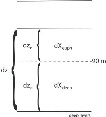
HAMOCC5.1 only allows biological production in the top 90 m of the water column. In az-level model this simply implies computing biological production in the layers that lie above this depth. In an isopycnic model layer thickness changes over time and space.

20

We thus redefined the original criterium and now test for changes in layer thickness at every time step of the biogeochemical model: in order for biological production to occur at least 10 m of an isopycnic layer must lie within the 90 m euphotic zone. The layer that contains the 90 m boundary is split virtually into a part above and one below the euphotic zone boundary and is assumed to be instantly well-mixed (Fig. 1). Changes

25

(12)

GMDD

2, 1023–1079, 2009

K. Assmann et al.

Title Page

Tables Figures

◭ ◮

Back Close

Full Screen / Esc

of the layer that lies in the euphotic zone.

X_new= Xold×d zd

+₍_X

old+d Xeuph)×d ze

d z (7)

whereX is any biogeochemical tracer, d X_euph the change inX due to biological pro-duction,d z is the total layer thickness andd z_e andd z_d the parts of the layer that lie in the euphotic zone and below it, respectively. The diagnosed values for primary and

5

export production follow the formulation for biological production and are also scaled to the top 90 m. Similarly, the part of the same layer that lies below the euphotic zone boundary experiences the remineralization processes that occur in the deep ocean resulting ind X_deep.

X_new= Xold×d ze

+₍_X

old+d Xdeep)×d zd

d z (8)

10

We used HAMOCC’s implicit sinking scheme with fixed sinking velocities, but ex-cluded massless layers from the routine. The 12-layer sediment model inex-cluded in HAMOCC 5.1 was used without amendment. It exchanges fluxes with the lowest ocean layer exceeding 0.5 m in thickness.

HAMOCC’s biogeochemical tracers are advected and mixed as passive tracers in

15

MICOM. MICOM uses a leap-frog time stepping scheme. For computational effi_ciency

ran the biogeochemical tracers on only one of its time levels and thus only every second physical time step. Therefore we corrected the global tracer budget for changes in layer thickness caused by time-smoothing between the two physical time levels to ensure tracer conservation.

20

2.3 Model configuration, initialisation and forcing

(13)

GMDD

2, 1023–1079, 2009

K. Assmann et al.

Title Page

Tables Figures

◭ ◮

Back Close

Full Screen / Esc

et al., 2003, Fig. 1b). At the equator the grid resolution is 2.4◦ zonally and 0.8◦ merid-ionally. With increasing latitude the grid cells are gradually transformed to have more isotropic metric scale factors in the horizontal directions. The grid spacing ranges from 60 km in the Arctic and Southern Oceans to 180 km in the subtropical gyres. In the ver-tical, the model has 35 layers of which the uppermost is a mixed layer with temporally

5

and spatially varying density. The potential densities of the isopycnal layers are in the range of 1030.12–1037.80 kg m−3.

The physical model is initialised from rest with temperature and salinity distribu-tions based on the January climatologies from Levitus and Boyer (1994) and Levitus et al. (1994), respectively. Nutrients and DIC/Alkalinity in HAMOCC were initalised

10

from global mean vertical profiles based on WOA05 (Boyer et al., 2006) and GLODAP (Sabine et al., 2005), respectively. The model was spun up for 950 years. The first 600 of these were performed with a monthly NCEP-based climatology (Kalnay et al., 1996). This does not include the synoptic and interannual variability necessary to obtain re-alistic sea ice distributions and surface mixing and mixed layers, and we switched to

15

repeated passes of the NCEP Reanalyses 1950–1999 for another 350 years of spin-up. The NCEP reanalysis data provide radiative fluxes and turbulent surface fluxes of momentum and heat, along with information on the ocean surface state (temperature and sea ice concentration). The forcing scheme and procedure proposed in Bentsen and Drange (2000) is used here. The scheme reproduces the reanalysis fluxes if the

20

model has the same surface state as in the reanalysis. These states will generally diff_er,

however, and the fluxes are modified accordingly. The turbulent fluxes are modified consistent with the bulk parameterization of Fairall et al. (1996) and long-wave radiative fluxes consistent with the Berliand and Berliand (1952) parameterization. Precipitation is directly provided by the NCEP reanalysis and the evaporation is calculated based

25

(14)

GMDD

2, 1023–1079, 2009

K. Assmann et al.

Title Page

Tables Figures

◭ ◮

Back Close

Full Screen / Esc

with thicker mixed layers (see Bentsen et al., 1999). For experiments forced by NCEP Reanalyses after 1948 this is reduced to 60 days for SSS and 180 days for SST to allow the development of surface SST and SSS anomalies, while still maintaining a realistic AMOC.

The model is initialised with a preindustrial atmospheric CO₂ level of 278 ppm

5

and is then allowed to evolve freely during the spin-up. It stabilises at a value of 286 ppm. We start our emission scenario runs in 1860 using values for anthro-pogenic CO₂ emissions from Boden et al. (2009). Since no gridded physical atmo-spheric forcing data exist prior to 1948, we use perpetual forcing with the NCEP year 1959 for the period 1860–1947. 1959 is both relatively neutral for both NAO

10

(see e.g. http://www.cru.uea.ac.uk/cru/climon/data/nao/) and ENSO (see e.g. http: //www.cdc.noaa.gov/people/klaus.wolter/MEI/), as well as being early in the NCEP pe-riod. This should ensure that air temperatures and Southern Ocean winds are still relatively close to preindustrial conditions. Prior to starting the emission simulations the model was run with year 1959 forcing, but no emissions for 20 years to avoid a

15

drastic change at the start of the emission simulation. Initially, four simulations were performed:

– CLIM: The reference simulation that continues the spin-up. Forced by NCEP year 1959 without CO₂emissions for the entire 1860–2007 period.

– CLIM+_{EMS: Forced by NCEP year 1959 for the entire 1860–2007 period, but with}

20

anthropogenic CO₂emissions from 1860 to 2007.

– SYN: Forced by NCEP Reanalyses 1948–2007 without CO₂emissions. Initialised from CLIM at the end of year 1947.

– SYN+_{EMS: Forced by NCEP Reanalyses 1948–2007 and including}

anthro-pogenic CO₂ emissions for this period. Initialised from CLIM+_{EMS at the end}

25

(15)

GMDD

2, 1023–1079, 2009

K. Assmann et al.

Title Page

Tables Figures

◭ ◮

Back Close

Full Screen / Esc

3 Model results and evaluation

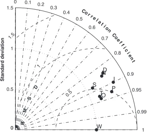
Since most observational data available was obtained over the last three decades we use an average of the years 1978–2007 of the SYN+_{EMS simulation for comparison}

to global climatologies. We summarise model performance in a Taylor diagramme (Fig. 2), and provide a more detailed discussion in the following sections.

5

3.1 Physical model

Amended versions of MICOM have been evaluated in several studies throughout its development particularly in the North Atlantic (e.g. Nilsen et al., 2003; Bentsen et al., 2004; Gao et al., 2004; Drange et al., 2005; Hatun et al., 2005, Lohmann et al., 2008). Here we present an evaluation of the main features of the physical model mainly to

10

provide a context for the biogeochemical tracer distributions.

Overall, the simulated circulation as well as the potential temperature and salin-ity fields are realistically described by the model. The model reproduces both global salinity S and potential temperature Θ_{distributions well, with a slighty better pattern}

representation for temperature (Fig. 2). Simulated distributions have larger normalised

15

standard deviations (STD), i.e. stronger gradients, than observed. This is likely due to MICOM not being very diff_{usive and to low exchange between the isopycnal layers}

and their outcropping region in the surface mixed layer across their diapycnal interface. Surface distributions for both salinity and temperature are close to the observed ones (Figs. 3 and 4). Since salinity is relaxed quite strongly to observations, SSS deviations

20

are generally below 0.2 psu. Notable exceptions from this are the estuaries/plumes of big rivers, especially in the Arctic, in whose vicinity the model overestimates salin-ity. Rather than explicitly prescribing river fresh water fluxes, MICOM uses a run off

scheme to route NCEP precipitation on land into the ocean. While this ensures fresh water conservation, it means that fresh water inputs from continents in the model do

25

(16)

GMDD

2, 1023–1079, 2009

K. Assmann et al.

Title Page

Tables Figures

◭ ◮

Back Close

Full Screen / Esc

path of the North Atlantic Current that leaves the North American coast too far North as is common in coarse resolution models. The resulting large heat loss may lead to low SSTs in the sub-polar gyre and northwestern sub-tropical gyre. The North Pacific and Kuroshio show a similar pattern. SSTs are generally too cold. A notable exception are the upwelling regions where overestimated temperatures indicate that the upwelling

5

strength is too weak.

Meridional sections in the Atlantic show that the model produces deep and bottom water masses that are too fresh and cold (Figs. 3 and 4). Simulated sub-surface and deep waters in the Greenland Sea are warmer and slightly fresher than observed, pos-sibly due to underestimated convection intensity in the model. The overly cold and

10

fresh waters in the Labrador Sea in our simulation stem from two origins: a Denmark Strait overflow where water appears to experience too little entrainment during its de-scent and local convection of overly fresh and cold surface waters in the Labrador Sea caused by misrepresentations in the course of the North Atlantic Current.

Overestimated Θ _{and S above 1000 m in the tropics and subtropics indicate weak}

15

replenishment of Sub-antarctic Mode Water (SAMW) and Antarctic Intermediate Water (AAIW). Water with the characteristically low salinity of AAIW is subducted to depths of up to 3000 m in the AAIW formation regions, because its temperatures are too low by 2.5◦C and thus its density allows it to sink to these depths. The source of this cold water can be found further South. While deep convection and formation of cold and saline

20

waters is only observed on Antarctic shelves, the water column of the deep Weddell Sea is only weakly stratified when using the surface as a refererence level for potential density. In fact, the choice of 2000 m as a reference level for our model density layers means that the observed stratification in this area is unstable (Fig. 5). This initially leads to overestimated vertical mixing in our model which erodes the Warm Deep Water

25

(17)

GMDD

2, 1023–1079, 2009

K. Assmann et al.

Title Page

Tables Figures

◭ ◮

Back Close

Full Screen / Esc

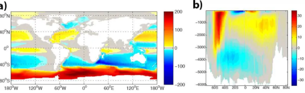
Central Intermediate Water (CIW) exported are colder than observed. Consequently, water upwelled in the southern limb of the Deacon Cell (Fig. 6a is too cold and leads to the excessive subduction of AAIW described above.

This process also leads to the relatively strong AABW cell of 14 Sv in the global meridional overturning circulation (Fig. 6a) since the deep AABW outflow is joined

5

by water which would normally exit the Southern Ocean as AAIW at much shallower depths. The model does, however, show a realistic North Atlantic overturning of 14 Sv. Major features of the horizontal circulation (Fig. 6b) are in general well-reproduced with an ACC strength of 150–160 Sv, a Weddell Gyre of 50 Sv (Beckmann et al., 1999), a Ross Gyre of 20–30 Sv (Assmann and Timmermann, 2005) and a North Atlantic

Sub-10

tropical and Sub-polar Gyres of 30–40 Sv.

3.2 Biogeochemistry

Correlations for all biogeochemical 3-D fields that we compared lie above 0.8 (Fig. 2). As for Θ _{and S simulated standard deviations are higher than observed by 10–35%}

again indicating that the model overestimates gradients in the distributions.

15

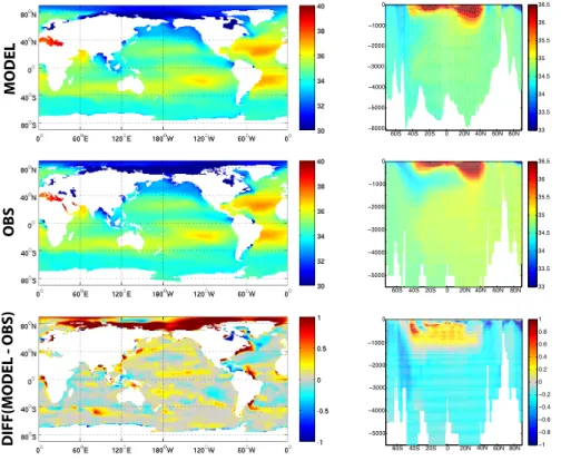
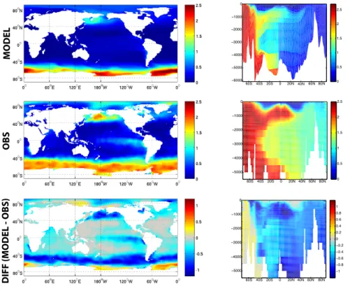
Phosphate is useful for a baseline assessment of the biogeochemical tracers since it is not aff_{ected by air-sea gas exchange. Its surface concentrations are generally low}

due to uptake during biological production. Higher deep ocean concentrations arise from the remineralisation of this biological matter after sinking out of the euphotic zone. Areas of higher surface phosphate are associated with upwelling, e.g., the Southern

20

Ocean and the Equatorial Pacific, or enhanced mixing, e.g. the North Pacific. Lower deep concentrations indicate areas of deep water formation like the North Atlantic.

Simulated surface phosphate concentrations are generally underestimated (Fig. 7). Exceptions are the Siberian shelves, where dissolution from the sediment increases concentrations, and the Southern Ocean below 60◦S. The weak upwelling in the model

25

(18)

GMDD

2, 1023–1079, 2009

K. Assmann et al.

Title Page

Tables Figures

◭ ◮

Back Close

Full Screen / Esc

is not included in our model and likely contributes to low phosphate concentrations in the model. The North Pacific and the Southern Ocean between 40◦ and 60◦ are the formation regions for intermediate waters that supply much of the low-latitude ocean with nutrients (Sarmiento et al., 2004). In our simulation surface phosphate concentra-tions in these regions are too low and the most obvious deviation from observaconcentra-tions.

5

Meridional sections in the Atlantic (Fig. 7) illustrate how the low simulated preformed surface concentrations are communicated into the intermediate water masses. Analy-sis of the physical fields showed that the model’s Antarctic Intermediate Water (AAIW) tongues are less pronounced than in observations. The subduction of low-salinity wa-ter that would normally contribute to AAIW to much greawa-ter depth aids the trapping of

10

nutrients in the Antarctic Marginal Seas and Antarctic Bottom Water (AABW) where the model overestimates nutrient concentrations. We will explore the relative roles of physics and biology for the preformed concentrations in the AAIW formation regions through sensitivity studies in Sect. 5.

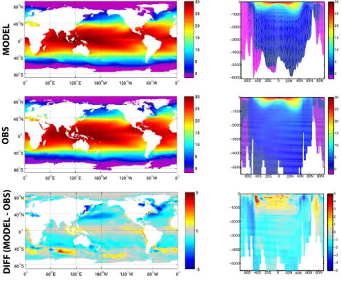
To first order, the global distribution of oxygen is a mirror image of the distribution of

15

nutrients. In addition, surface oxygen concentrations bear the imprint of temperature dependent dissolution with higher concentrations in cold high-latitude waters. Accord-ing to the Taylor diagramme (Fig. 2) oxygen, along with potential temperature, is the tracer that the model simulates best. A comparison of modelled and observed surface oxygen distributions (Fig. 8) confirms this, as deviations are small except in the Arctic

20

and Southern Oceans. The modelled sea ice extent in the Southern Ocean is too large in summer and thus prohibits air-sea gas exchange. Also, our model – as most other biogeochmical ocean models – treats sea ice as an impregnable lid to air-sea fluxes, which it may not be. In addition, observations are generally summer-biased in polar regions. This may lead to higher observed oxygen concentrations since they are

domi-25

(19)

GMDD

2, 1023–1079, 2009

K. Assmann et al.

Title Page

Tables Figures

◭ ◮

Back Close

Full Screen / Esc

and nutrient supply which lead to low biological production and remineralisation of sink-ing organic matter. However, it also indicates that our model is not prone to the nutrient trapping at the Equator commonly seen in biogeochemical ocean models (Aumont et al., 1999). Low AAIW oxygen concentrations confirm the weak formation rates of this water mass in the model.

5

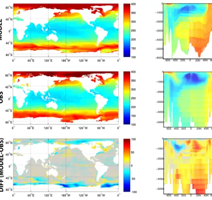
Dissolved Inorganic Carbon (DIC, Fig. 9) shows in principle the same deviations from the observations as phosphate, but performs worse in the Taylor diagramme since it is also aff_{ected by air sea gas exchange and opal/CaCO}

3 production. Again, the main

feature is the trapping of carbon in the far Southern Ocean and low carbon in the NADW.

10

Global mean values for biological production are within observation-based estimates. Mean global primary production is at 48.5±2.0 Gt C yr−1, POC export production at 12.4±0.53 Gt C yr−1, calcium carbonate export at 0.91±0.04 Gt C yr−1 and silicate ex-port at 157.6±7.2 Tmol Si yr−1(Treguer et al., 1995). Our value for global primary pro-duction agrees well with a satellite-based estimate of 48 Gt C yr−1 by Behrenfeld et

15

al. (2006) and is within the range of 35 to 70 Gt C yr−1 given by Carr et al. (2006). Export production is well within the observational estimates which range from 11 to 22 Gt C yr−1 (Eppley and Peterson, 1979; Laws et al., 2000; Schlitzer, 2000), and markedly higher than that in other contemporary coupled climate carbon cycle mod-els (Schneider et al. 2008).

20

The global distribution of primary and export production (Fig. 10) shows maxima in the North Atlantic and Pacific and in the coastal and equatorial upwelling regions, as expected (e.g. Schneider et al., 2008, Fig. 6). Biological production in the shallow shelf areas is underestimated as in most global models due to the lack of resolution and nutrient inputs by rivers and run-off_{. Due to the low nutrient supply to the North}

25

(20)

GMDD

2, 1023–1079, 2009

K. Assmann et al.

Title Page

Tables Figures

◭ ◮

Back Close

Full Screen / Esc

to the simulated summer sea ice edge. We will explore possible reasons for this in a series of sensitivity studies in Sect. 5.

4 Air-sea fluxes and the uptake of anthropogenic CO₂

There is a steady ocean carbon uptake of 0.05±0.006 Gt C yr−1 in the reference sim-ulation, CLIM, which indicates that this simulation has reached equilibrium after the

5

spin-up (Fig. 11a). In the simulation forced by NCEP Reanalyses, SYN, annual ocean carbon fluxes vary between−0.2 and 0.3 Gt C yr−1. Notable is a positive trend in the carbon fluxes in SYN after the late 1990s indicating that changes in the physical sys-tem reduce the ocean’s ability to take up carbon. In the equivalent simulation including emissions, SYN+_{EMS, the increase in ocean carbon uptake slows after this point,}

10

while uptake in the CLIM+_{EMS simulation continuously forced by NCEP year 1959}

increases more sharply due to an acceleration in anthropogenic emissions. Thus our model results agree with recent findings of a weakening of the ocean carbon sink due to a climate-carbon cycle feedback (Schuster and Watson, 2007; Schuster et al., 2009; LeQu ´er ´e et al., 2007; Metzl, 2009).

15

Air-sea carbon flux climatologies based on observations estimate an ocean carbon uptake of 2.2±0.5 Gt C yr−1 for 1995 (Takahashi et al., 2002) and in an updated ver-sion 1.4±0.7 Gt C yr−1(2.0±0.7 Gt C yr−1anthropogenic uptake) for 2000 (Takahashi et al., 2008). Simulated ocean uptake for these years is 2.8 Gt C yr−1 and 2.7 Gt C yr−1, respectively, and thus just outside upper bounds for the observational values. It is,

20

however, worth noting that Takahashi et al. (2008) assume a preindustrial ocean car-bon source of 0.4 Gt C yr−1 which brings their estimate of anthropogenic carbon up-take closer to ours since the simulated 2000 flux without emissions in SYN is only 0.06 Gt C yr−1.

A comparison of the observed year 2000 climatology and the simulated fluxes for the

25

(21)

GMDD

2, 1023–1079, 2009

K. Assmann et al.

Title Page

Tables Figures

◭ ◮

Back Close

Full Screen / Esc

rates discussed in Sect. 3.1. In addition, uptake in the high latitude sink regions of the North Pacific, North Atlantic and Southern Ocean is generally overestimated. Reasons for this are likely associated with the artificially large vertical mixing in the model which allows fast subduction of carbon taken up particularly in winter and overestimated ex-port production in the Southern Ocean. The fact that MICOM has a bulk mixed layer

5

probably also contributes to this phenomenon: carbon taken up at the ocean surface is instantaneously mixed with a volume of water that particularly in winter is large. The resulting changes to surfacepCO₂are consequently small and further uptake is easily possible.

The Southern Ocean is the region with the largest disagreement between model and

10

climatology. When the area south of 56◦S is excluded, the correlation between simu-lated and observation-based air-sea fluxes and∆_p_CO

2patterns improves from 0.38 to

0.73 for∆_p_CO

2and from 0.55 to 0.68 for the air sea fluxes. This is particularly striking

for∆_p_CO

2 since a thick perennial sea ice cover in the model prohibits outgassing in

the central Weddell Sea and leads to excessively high surface∆_CO

2values. However,

15

the observed climatology is likely summer-biased in this region which would lead to un-derestimated∆_p_CO

2. There also is as yet no parametrisation of carbon fluxes through

sea ice available for large-scale models. Observations indicate that these fluxes are large (Semiletov et al., 2004), but most ocean carbon cycle models represent sea ice as an impregnable lid making the interpretation of their results in sea-ice covered areas

20

diffi_cult.

Using NCEP Reanalyses after 1948 leads to an atmospheric CO₂ about 2 ppm higher than in the experiment that was continuously forced with NCEP year 1959 (Fig. 11b). All models of the Coupled Climate Carbon Cycle Model Intercomparison Project (C4MIP) have a carbon cycle-climate feedback of less than 15 ppm in 2006

25

(Friedlingstein et al., 2006) and this small eff_{ect is thus not unreasonable for a}

(22)

GMDD

2, 1023–1079, 2009

K. Assmann et al.

Title Page

Tables Figures

◭ ◮

Back Close

Full Screen / Esc

carbon model and a representation of the “pioneer eff_{ect” which made the land a}

sig-nificant carbon source during this period (Houghton, 1999). Towards the end of the 20th century the simulated increase exceeds that observed, indicating a weakening of the ocean sink and a change of the land from source to sink. Of the 242.7 Gt C emitted between 1860 and 1994, the ocean in our model takes up 90 Gt C, leaving

5

152.7 Gt C in the atmosphere. Both of these numbers are smaller than those deduced from observations by Sabine et al. (2004) due to the lack of the net land source in the model.

The column inventory of anthropogenic CO₂ (Fig. 13) agrees well in pattern and magnitude with that deduced from observations by Sabine et al. (2004). Column

in-10

ventories that exceed those of the observations may both be due to overestimated ventilation of the deep basins in the model and inaccuracies of the C* method used to deduce anthropogenic CO₂ from the available observations (Matsumoto and Gruber, 2005). Underestimated column loads of anthropogenic CO₂in the tropical Atlantic can be explained both by the weak renewal of AAIW in the model and by the fact that our

15

simulation misses emissions due to the “pioneer” eff_{ect early in the emission scenario}

which would have had time to penetrate further into the ocean interior.

5 Sensitivity studies

One of the most striking deviations from observations in the model is the large bio-logical production and the excessively high nutrients in the Southern Ocean, an area

20

known as a HNLC-region (High Nutrient Low Chlorophyll). Biological production in the Southern Ocean is primarily limited by light and iron (e.g. Martin, 1990). We thus fo-cus our sensitivity studies exploring the origin of the artificially large Southern Ocean primary production on these factors. We ran each of the sensitivity simulations for the NCEP period from 1948–2007 with anthropogenic CO₂ emissions starting from year

25

1947 of the CLIM+_{EMS simulation, much like the setup of SYN}+_{EMS simulation. We}

(23)

GMDD

2, 1023–1079, 2009

K. Assmann et al.

Title Page

Tables Figures

◭ ◮

Back Close

Full Screen / Esc

SYN+_{EMS. Since the model has not been run to equilibrium for each of these 60 year}

long simulations, the diff_{erences shown are indicative only of the sign of the changes}

and the relative magnitude, but not of the final magnitude of the induced changes and total feedback on the carbon cycle. The following sensitivity experiments were con-ducted:

5

– IRON: Biological production in the model is phosphate, nitrate and iron co-limited by the expression

nutrient=_min

P O4,

NO₃

R_N_:_P,

Fe

R_Fe:_P

where R_Fe:P = 3.×10−6 ×RC:P , RC:P = 122 and RN:P = 16, according to

Redfieldian stoichiometry. To enhance iron limitation we usedR_Fe:_P =₅_._×₁₀−6_×

10

RC:P globally in this sensitivity study. Sarthou et al. (1997) derived an iron to

carbon uptake ratio ofR_Fe:_C =₃_.₄₇_×₁₀−6_{from observations in the Indian Sector}

of the Southern Ocean.

– ABS: In our standard model version the entire mixed layer (or the part that is within the 90 m euphotic zone) receives the full incoming short wave radiation.

15

To reduce biological production in regions with deep mixed layers in spring, the mixed layer is split virtually into a 20 m thick surface layer and the rest below this up to a maximum euphotic zone depth of 90 m. Only the top 20 m receive the full incoming short wave radiation, while the short wave radiation incident on the lower part of the layer has been attenuated by absorption in the top 20 m.

20

– DIAPYC: One issue in isopycnal models are layers that outcrop at the surface. In order to represent surface processes a mixed layer with varying density is added in MICOM which contains these outcrops. There is thus an artificial diapycnal boundary between the isopycnal layers and their surface expression. Exchange across this boundary happens by changes in mixed layer thickness due to surface

(24)

GMDD

2, 1023–1079, 2009

K. Assmann et al.

Title Page

Tables Figures

◭ ◮

Back Close

Full Screen / Esc

buoyancy fluxes and diapycnal mixing as used between the standard isopycnal layers. To account for the fact that fluxes between the mixed layer and the isopyc-nal layer are isopycisopyc-nal rather than diapycisopyc-nal we increased the parameterCin the expression for the background diff_usivity _ν

bin Eq. (5) for the layer directly below

the mixed layer by a factor of 10.

5

In both IRON and ABS, export production decreases in a broad band between 40◦S and the sea ice edge (Fig. 14). In both cases this coincides with an increase in phate concentrations in this area (Fig. 15) suggesting that the underestimation of phos-phate concentration seen in Fig. 7 is due to excessive export production. However, the globally enhanced iron limitation leads to a significant and unrealistic increase in

sur-10

face phosphate throughout the Pacific, South Atlantic and Indian Ocean. No change in phosphate is seen in IRON in the North Atlantic and Indic where large dust input from the Sahara leads to nitrate rather than iron limitation. Consequently, there is no change in export production in the North Atlantic in IRON, while there is a reduction in both the North and Equatorial Pacific.

15

In ABS increased surface phosphate (Fig. 15) in the North Pacific and Atlantic coin-cides with reduced export production (Fig. 14). While the former is a desirable improve-ment of the model results (Fig. 7), the latter is already underestimated in the standard model version. This indicates that we are possibly missing additional nutrient sources in these areas. The model only receives fresh water, but not the accompanying

nu-20

trient fluxes from the large Siberian rivers. These are suggested to be a significant source of nutrients in the North Atlantic (Jones et al., 2003), in addition to nutrient rich waters from the North Pacific that enter the Arctic and North Atlantic through Bering Strait. In the North Pacific, tidal mixing has been suggested as an important factor for transporting nutrient-rich intermediate waters into the surface layer to sustain vigorous

25

(25)

GMDD

2, 1023–1079, 2009

K. Assmann et al.

Title Page

Tables Figures

◭ ◮

Back Close

Full Screen / Esc

needed to make the highly nutrient-rich deep and intermediate waters of the North Pacific accessible for biological production in the surface layer. In contrast, there is no significant eff_{ect in DIAPYC in the North Atlantic where waters directly underlying the}

surface are low in nutrients. Similarly to the North Pacific, enhanced diapycnal mixing between the mixed layer and sub-surface enhances both surface phosphate and export

5

production in the Southern Ocean, extending both to just north of 40◦S. This northward extension brings our model distributions closer to observed ones and highlights the im-portance of exchange between the surface and intermediate as well as mode waters in this region. The strong increase of export production further south in DIAPYC may in part be due to the overestimated deep nutrient concentrations south of the ACC.

10

Evaluating the vertical phosphate distribution along a meridional section in the At-lantic, we found that while simulated concentrations south of the ACC are overesti-mated, concentrations in the AAIW and NADW are too low (Fig. 7). All sensitivity studies remedy the distribution in the Southern Atlantic by lowering nutrient concentra-tions in both CDW and AABW and increasing them in the AAIW and SAMW (Fig. 16).

15

Decreasing export production in the IRON and ABS experiments leads to an increase of pre-formed surface phosphate in those regions where AAIW and SAMW are sub-ducted. The decrease of fast-sinking detritus that remineralises below the intermediate waters lowers phosphate concentrations south of the ACC and finds a surface ex-pression in a decrease of phosphate concentrations where these deep waters upwell

20

underneath sea ice in the Weddell Sea. The existence of the same pattern in DIAPYC albeit with a lesser reduction in the south indicates that the main factor for the enhanced intermediate water concentrations is indeed the increased northward extension of both pre-formed nutrients and biological production.

While the enhanced mixing in DIAPYC does lead to a 2.3 Pg C yr−1increase in POC

25

(26)

GMDD

2, 1023–1079, 2009

K. Assmann et al.

Title Page

Tables Figures

◭ ◮

Back Close

Full Screen / Esc

in atmospheric CO₂ over the 60 yr time period of the sensitivity experiment. The 2.5 Pg C yr−1 reduction in export production in the ABS experiment leads to an atmo-spheric CO₂increase of 14.4 ppm. Even though changes in export production from the reference run are almost constant over time (Fig. 17a), it takes around 20 years for the initial reaction of global ocean CO₂ uptake (Fig. 17b) to subside. Especially in ABS

5

and IRON the reduction of summer pCO₂ drawdown due to the abrupt reduction in biological production initially leads to carbon outgassing. As the ocean surface adjusts to the new annual cycle some of this carbon is taken up again aided by the simulated increase in export production after 1980.

6 Discussion

10

We have presented a new ocean carbon cycle model consisting of the isopycnic ocean model MICOM and the biogeochemistry model HAMOCC. After a thorough evaluation we conclude that it is well-suited for global carbon cycle studies. Previous attempts to use isopycnic ocean models as the physical part of ocean carbon cycle models are scarce and had their problems (Drange, 1997; Haigh et al., 2001). However, continuing

15

development of layered ocean models now has improved performance so much that our attempt has been more successful. The strength of an isopycnic vertical coordinate lies in it being a close approximation to the surfaces on which tracer transport in the interior ocean actually takes place. We find that our model reproduces, e.g., the invasion of anthropogenic carbon into the interior ocean extremely well.

20

A disadvantage of the isopycnic coordinates lies in the need to use a mixed layer of varying density to handle layer outcropping at the ocean surface and air-sea exchange processes. MICOM uses a bulk mixed-layer which implies that vertical resolution at the ocean surface is limited. It is therefore not particularly suited to detailed surface-ocean ecosystem studies that require a highly resolved euphotic zone. A relatively

25

(27)

GMDD

2, 1023–1079, 2009

K. Assmann et al.

Title Page

Tables Figures

◭ ◮

Back Close

Full Screen / Esc

coordinate was indeed in representing biological processes in the euphotic zone, e.g., phytoplankton growth and light absorption. A hybrid-coordinate model like HYCOM (Bleck, 2002) where the surface layer is split into closely spacedz-levels is the better tool where dedicated ecosystem studies are concerned.

A series of sensitivity studies were performed, initially with the purpose of exploring

5

the origin of several model shortcomings like the vigorous biological production in the Southern Ocean. A result common to all of these is the importance of the distribu-tion of preformed nutrients in the Southern Ocean on the global nutrient distribudistribu-tion as highlighted by Sarmiento et al. (2004) and Marinov et al. (2006). The overesti-mated biological production in our reference model experiment depletes surface

nutri-10

ents leading to low nutrient concentrations in the AAIW. Instead, these nutrients sink into the upwelling CDW where they are remineralised and trapped within the unpro-ductive southern loop of the MOC (Marinov et al., 2006). Reducing this export by both enhanced iron limitation and a more sophisticated light absorption scheme leads to a reduction in phosphate in this southern loop and an increase in nutrients in mode and

15

intermediate waters. While enhanced diapycnal mixing between the mixed layer and the isopycnic layer immediately below leads to an increase in export production in the Southern Ocean, it produces the same pattern as the biogeochemical changes in the phosphate distribution, since it is also a mechanism that increases surface nutrients in the mode and intermediate water formation regions.

20

From the large-scale surface increase in phosphate in IRON we conclude that this approach is either too simplistic or that iron is not at the root of the problem. Our standard carbon to iron ratio appears to be realistic (Sarthou et al., 1997) and modelled iron concentrations agree with available observations (Moore and Braucher, 2008). If iron were to be the solution, uptake ratios would have to vary with either species

25

(28)

GMDD

2, 1023–1079, 2009

K. Assmann et al.

Title Page

Tables Figures

◭ ◮

Back Close

Full Screen / Esc

As discussed above most of the challenges in adapting an ocean biogeochemistry module for use with an isopycnic coordinate lay in making it suitable for use with a bulk mixed layer. An important point here was light absorption. While we explored various parametrisations during model development, we settled on a fairly simple formulation for our reference run. The ABS sensitivity run shows that this was maybe too simple,

5

but also that the improvement of this process made a large impact on our results and will be used in further studies.

In the evaluation of our model results the eff_{ect of sea ice on biogeochemical}

pro-cesses and its representation as an impregnable lid was touched upon several times. There is mounting evidence that sea ice is not simply a lid to air-sea exchange and

bi-10

ology (Semiletov et al., 2004), but more sophisticated parametrisations are necessary to include this in ocean carbon cycle and Earth System Models. Motivated by exces-sive DIC values under sea ice particularly in the Southern Ocean, we allowed some exchange through sea ice by limiting the maximum sea ice concentration in HAMOCC experiences to 0.5. More permeable sea ice would allow outgassing of some of this

15

carbon and some biological production, attempting to counteract the overestimated summer sea ice extent in the Southern Ocean. After a 60 year simulation the eff_ects

are still largely confined to sea ice covered areas. Changes to atmospheric CO₂, ocean carbon uptake and export production are not significant. There is a substantial reduc-tion in phosphate in Arctic surface waters that extend into the Labrador Sea where it is

20

subducted into the deep ocean. This implies that Arctic waters play an important role in North Atlantic nutrient supply. Missing nutrient inputs from Arctic rivers (e.g. McClel-land et al., 2006) and an underestimated Pacific water layer (Falck et al., 2005; Jones et al., 2003) may explain the low nutrient concentrations and biological production in these regions in our model.

25

(29)

GMDD

2, 1023–1079, 2009

K. Assmann et al.

Title Page

Tables Figures

◭ ◮

Back Close

Full Screen / Esc

the climate system’s response to anthropogenic CO₂ emissions lie well within the bounds of other coupled carbon cycle-climate models (Tjiputra et al., 2009). Work on a new model version currently in progress includes some of the parametrisations explored in our sensitivity studies as well as a parametrization of vertical mixing that circumvents the issue of unstable Southern Ocean sub-surface stratification with a

5

2000 m reference pressure.

Acknowledgements. This study at the University of Bergen and Bjerknes Centre for Climate

Research is supported by the EU-FP6 integrated project CarboOcean (grant nr. 511176), and the Research Council of Norway funded projects MerClim and CarbonHeat. This is publication

10

no. xxxx from the Bjerknes Centre for Climate Research.

References

Arakawa, A. and Lamb, V. R.: Computational design of the basic dynamicl process of the UCLA general circulation model, Meth. Comput. Phys., 16, 173–283, 1977.

Archer, D.: Fate of fossil fuel CO2 in geologic time, J. Geophys. Res., 110, C09S05,

15

doi:10.1029/2004JC002625, 2005.

Archer, D. and Maier-Reimer, E.: Eff_{ect of deep-sea sedimentary calcite preservation on} atmo-spheric CO2concentration, Nature, 367, 260–263, 1994.

Archer, D., Winguth, A., Lea, D., and Mahowald, N.: What caused the glacial/interglacial atmo-sphericpCO2cycles? Rev. Geophys., 38, 2, 159–190, 2000.

20

Assmann, K. M. and Timmermann, R.: Variability of dense water formation in the Ross Sea, Ocean Dynam., 55, 68–87, 2005.

Aumont, O., Orr, J. C., Monfray, P., Madec, G., and Meier-Reimer, E.: Nutrient trapping in the Equatorial Pacific: the ocean circulation solution, Global Biogeochem. Cy., 13(2), 351–369, 1999.

25

(30)

GMDD

2, 1023–1079, 2009

K. Assmann et al.

Title Page

Tables Figures

◭ ◮

Back Close

Full Screen / Esc

Bacastow, R., and Maier-Reimer, E.: Ocean-circulation model of the carbon cycle, Clim. Dy-nam., 4, 95–125, 1990.

Beckmann, A., Hellmer, H. H., and Timmermann, R.: A numerical model of the Weddell Sea: large scale circulation and water mass distribution, J. Geophys. Res., 104(C10), 23375– 23391, 1999.

5

Behrenfeld, M. J., OMalley, R. T., Siegel, D. A., et al.: Climate-driven trends in contemporary ocean productivity, Nature, 444, 752–755, 2006.

Bentsen, M., Evensen, G., Drange, H., and Jenkins, A. D.: Coordinate Transformation on a Sphere Using Conformal Mapping, Mon. Weather Rev., 127, 2733–2740, 1999.

Bentsen, M. and Drange, H.: Parameterizing surface fluxes in ocean models using the

10

NCEP/NCAR reanalysis data, RegClim General Technical Report No. 4, Norwegian Insti-tute for Air Research, 149–158, 2000.

Bentsen, M., Drange, H., Furevik, T. and Zhou, T.: Simulated variability of the Atlantic merid-ional overturning circulation, Clim. Dynam., 22, 701–720, 2004.

Berliand, M. and Berliand, T.: Determining the net long-wave radiation of the earth with

consid-15

eration of the eff_{ect of cloudiness, Isv. Akad. Nauk. SSSR Ser. Geofis. 1, 1952.}

Bleck, R. and Smith, L. T.: A Wind-Driven Isopycnic Coordinate Model of the North and Equa-torial Atlantic Ocean, 1. Model Development and Supporting Experiments, J. Geophys. Res., 95(C3), 3273–3285, 1990.

Bleck, R.: An oceanic general circulation model framed in hybrid isopycnic- cartesian

coordi-20

nates, Ocean Model , 4, 55–88, 2002.

Bleck R., Rooth, C., Hu, D., and Smith, L. T.: Salinity-driven Thermocline Transients in a Wind- and Thermohaline-forced Isopycnic Coordinate Model of the North Atlantic, J. Phys. Oceanogr., 22, 1486–1505, 1992.

Boden, T. A., Marland, G., and Andres, R. J.: Global, regional, and national CO2 emissions.

25

Trends: A compendium of data on global change, Carbon Dioxide Information Analysis Cen-ter, US Department of Energy, Oak Ridge, TN, USA, doi:10.3334/CDIAC/00001, 2009. Bolin, B., and Eriksson, E.: Changes in the carbon dioxide content of the atmosphere and sea

due to fossil fuel combustion, in: Th eatmosphere and the sea in motion, Rossby Memorial Volume, edited by: Bolin, B., Rockefeller Inst., New York, 130–142, 1957.

30