Methods Providing Good Conditioning of Model
Identification Task in Immune Inspired,
Steady-State Controller of an Industrial Process
K. Wojdan
∗K. Swirski
†M. Warchol
‡M. Maciorowski
§Abstract—Methods which provide good condi-tioning of model identification task in immune in-spired, steady-state controller SILO (Stochastic Im-mune Layer Optimizer) are presented in this paper. These methods are implemented in a model based op-timization algorithm. The first method uses a safe model to assure that gains of the process’s model can be estimated. The second method is responsible for elimination of potential linear dependences between columns of observation matrix. Moreover new results from one of SILO implementation in polish power plant are presented. They confirm high efficiency of the presented solution in solving technical problems.
Keywords: steady-state control, model identification, adaptation, artificial immune system
1
Introduction
Control and optimization of the steady state of industrial processes have been taken in a numerous research works and implementations. Industrial processes which take place in a large scale plants, with high level of complex-ity, are characterized by large number of control inputs, outputs and disturbances, long time of process response for control change, essentially non-linear characteristics and impossible to omit cross transforms. Classic control systems based on PID (Proportional Integral Derivative) controllers are not able to perform optimal control of such processes.
Methods based on predictive control algorithms with re-ceding horizon [3] are the most common solutions for advanced control of industrial process. In a multilayer structure of control system [3] an advanced control layer computes control vector, which is a set-point vector for a base control layer. An MPC (Model Predictive Control)
∗K. Wojdan is with the Warsaw University of
Technol-ogy, Institute of Control and Computation Engineering, Poland,
†K. Swirski is with the Warsaw University of Technology,
Insti-tute of Heat Engineering, Poland,[email protected] ‡M. Warchol is with the Warsaw University of
Technol-ogy, Institute of Control and Computation Engineering, Poland,
§M. Maciorowski is with Transition Technology, Poland, [email protected]
controller, based on the knowledge stored in a dynamic model, computes control vectors in consecutive moments
x(k), x(k+1), ..., x(k+Nu-1). This control trajectory
minimizes the difference between estimated process’s out-puts and demand output values in consecutive moments. Despite numerous advantages of MPC controllers there are some important disadvantages. Implementation of MPC controllers is expensive. Long lasting and labour-consuming parametric tests have to be done to create a dynamic, mathematical model. Honeywell experts have calculated that the cost of creating a dynamic model vary from USD250 to USD1000 for each, single dependence between one input and one output of the process [2]. Another disadvantage of predictive control methods is an insufficient adaptation to process’s characteristics changes. These changes are considered in a long-term horizon, like months and years, resulting from wearing or failure of devices, rebuilding of industrial system, changes of chemical properties of components used in a process or external conditions changes (e.g. seasonality). The eas-iest way to consider these changes is a manual, periodic update of the model based on most recent identification experiments of the process. However, this is not a satis-fying solution. Implementation of an adaptation method in a MPC controller is a more desired approach. This solution is related with some difficulties:
• Estimation of model’s parameters when there is an insufficient changeability of noised signals,
• Estimation of model’s parameters in closed loop op-eration,
• High computer resources usage in on-line operation,
• Possibility of linear dependences in an observation matrix, which consists of process measurements.
immune system of living creatures. SILO can be used to control processes, characterized by fast but rare distur-bance changes, or processes where disturdistur-bances change continuously but the rate of changes is essentially slower than the dynamics of the process. In the first case con-trol quality in transition states depends on a base concon-trol layer. In industrial plants which fulfill above-mentioned condition, SILO can be a low cost (in an economic mean-ing) and effective alternative for MPC controllers. It re-sults from:
• There is no need to perform identification experi-ments of the process manually;
• There is no need to createa prioria dynamic, math-ematical model of the process. It results in a signif-icant reduction of work time of high qualified engi-neers;
• Consideration of higher number of process operat-ing points. SILO automatically learns the process and adapts to current operating point. SILO can be forced to higher precision of adaptation by defi-nition of more narrow ranges of process’s signals, in which linear approximation is sufficient. In the case of MPC controllers number of such areas (i.e. fuzzied partitions) is limited by amount of labor related with parametric tests;
• Immune inspired efficient adaptation algorithm which is able to acquire knowledge about the pro-cess.
2
Immune structure of SILO
The structure of immune optimizer was described in [4, 5]. In this chapter the immune structure of SILO is briefly reminded. Vector x represents control inputs, vector y
represents process outputs (y) and vector z represents measured disturbances. An analogy between an immune system and SILO is presented below:
Pathogen – Measured and non-measured distur-bances,
B cell – Historical static process responce to a control change,
Antibody - effector part – Optimal control vector change,
Antibody - antigen binding side – Current process state (current values of x, y and z vectors), stored in a B cell.
In the SILO system the B cell represents values ofx,yand
z vectors before and after a control change. Thus B cell represents static process responce to a control change.
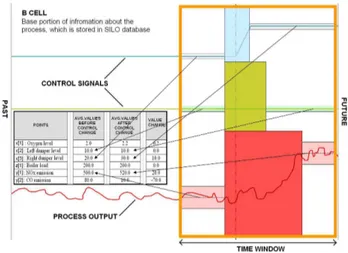
Figure 1: Time window of a B cell.
One should notice that the B cell represents only such process states, in which measured disturbanceszare con-stant. The example of a B cell is presented in Fig. 1. The formal definition of thek-th B cell is presented below:
Lk=bx¯k,px¯k,by¯k,py¯k,z¯k,
where: bx¯k – average values of control signals measured
before control change,px¯k– average values of control
sig-nals measured after control change,by¯k – average values
of process outputs measured before control change,py¯k –
average values of process outputs measured after control change, ¯zk – average values of measured disturbances.
In later considerations the following increases of control points and process outputs will be useful
∆xk =px¯k−bx¯k,
∆yk =py¯k−by¯k.
In a SILO system, an antigen which is located on a pathogen’s surface, is represented by current process state vectorA= [xa, ya, za]. Antibody (historical process state
stored in a B cell) binds the antigen only when a current process state is similar to the process state stored in a B cell that has created the antibody. Affinity between B cellLk and antigenAis defined in the following way:
µ(Lk, A) = nx
Y
i=1
gixb b
¯
xki, x a i
!
×
nx
Y
i=1
gixp p
¯
xki, x a i
!
×
×
ny
Y
i=1
gyib b¯
yik, y a i
!
×
ny
Y
i=1
gyip p¯
yik, y a i
!
×
×
nz
Y
i=1
giz z¯ k i, z
a i
!
where ∀x1, x2∈ ℜ g(x1, x2)∈ {0,1}. The antibody
binds the antigen only whenµ(Lk, A) = 1. The example
ofg(x1, x2) function is presented below:
g(x1, x2) =
0 if |x1−x2|> ε
3
Optimization algorithm
SILO consists of two main, independent modules – a learning and an optimization module. The operation of both modules is wider discussed in [4, 6]. The learning module performs on-line analysis of current and histori-cal values of elements of x,y and zvectors and searches for time windows which fulfill the criteria of being a B cell. When the module finds a time window which meets those requirements, then the recognized B cell is saved in a database, which represents the knowledge about the process. At least one control signal must change, to trans-form a time window into a B cell. During normal op-eration of a plant there are frequent changes of control inputs. Thus, the process of creating B cells is continu-ous. SILO updates its knowledge about the process all the time. It ensures constant adaptation to changeable operation conditions. Control changes can be caused by an operator, a base control layer or by an optimization module of SILO.
The optimization module operates in closed-loop. Based on current process state, B cells from immune memory and quality indicator coefficients, the optimization mod-ule computes an optimal increment of the control vector. The quality indicator’s value depends onxandyvectors. Equation 1 defines acontrol form of quality indicator
J =
nx
X
k=1
h
αk |xak−x s k| −τ
lx k
++
+βk(|xak−x s k| −τ
sx k )
2 +
i
+
+
ny
X
k=1
γk
|ya
k−ysk| −τ ly k
++
+δk(|yak−y s k| −τ
sy k )
2 +
i
(1) where: αk – linear penalty coefficient for k-th control
variable, βk – square penalty coefficient for k-th
con-trol variable,γk – linear penalty coefficient for k-th
op-timized output, δk – square penalty coefficient for k-th
optimized output, τlx
k – width of insensitivity zone for
linear part of penalty for k-th control variable, τsx k –
width of insensitivity zone for square part of penalty for
k-th control variable,τkly – width of insensitivity zone for linear part of penalty for k-th optimized output, τksy – width of insensitivity zone for square part of penalty for
k-th optimized output, (·)+ – ”positive part” operator
(x)+ = 1
2(x+|x|), x s
k – demand value for k-th control
variable, ys
k – demand value for k-th optimized output.
One can easy transform this equation to an economic formof quality indicator. In such case optimization mod-ule will perform on-line economic optimization of process operating point [6].
Optimization method is discussed in [5, 6]. The opti-mization period is defined as a the time range between
Figure 2: Layers of optimization algorithm.
control vector changes. This time is not shorter than time needed to reach steady-state of process outputs, af-ter control change. In case of combustion process in large scale power boiler, this time period vary from 5 to 15 min-utes.
Optimization algorithm operates in one of three optimiza-tion layers. In each layer a different optimizaoptimiza-tion algo-rithm is used to compute an optimal control vector in-crement that minimizes quality indicator. An algorithm that lets SILO switch between layers is a key algorithm of this solution (refer to Fig. 2). Activation of particular layer depends on SILO’s knowledge and current process’s state.
Stochastic optimization layer corresponds with stochastic exploration of the solutions’ space. It is being executed when SILO has no knowledge about the process or when the knowledge about the process is insufficient. The solu-tion found in this layer is a starting point for optimizasolu-tion in layers that use a process’s model. By analogy to an im-mune system this layer represents the primary response of the immune system [1].
Optimization on the global model layer – this layer uses general knowledge about an optimizing process to com-pute an optimal increment of control vector. An automat-ically created steady-state model (2), used in this layer, aggregates knowledge about basic process dependences. This layer is being executed when SILO does not have sufficient knowledge about the process and thus SILO is not able to create a mathematical model that represents static process dependences in the neighborhood of the current process’s operating point. The newest portions of knowledge (B cells) from different process’s states are being used to create a global model.
This layer corresponds with exploitation of solutions’ space. By analogy to immune system this layer repre-sents secondary immune response [1].
Methods which provide good conditioning of model iden-tification task, are implemented in global and mixed model based optimization layers. These methods are re-sponsible for maintenance of a reliable model of the pro-cess.
3.1
Model
Identification
in
mixed
and
global model layers
In optimization on the mixed model layer a mathemati-cal, linear model of the process is constructed. Informa-tion stored in g youngest global B cells and l youngest
local B cells are used to construct this model. The set of global B cells represents all B cells stored in immune memory. The set of local B cells represents B cells which fulfill affinity conditions. For those B cellsLk, it holds:
µ(Lk, A) = 1,
whereA= [xa, ya, za] is a current process state.
A linear static model of the process is defined below: ∆y= ∆xK, (2) where ∆x = [∆x1,∆x2, . . . ,∆xnx], ∆y =
[∆y1,∆y2, . . . ,∆yny] and K is a gain matrix.
Co-efficients of a K matrix are estimated using the least square method. Analytical solution (4) of normal equation (3) is presented below:
(W +µI)K= (V +µM) (3)
K= (W +µI)−1
(V +µM) (4) where:
V =η∆XT
L∆YL+ϑ∆XGT∆YG, W =η∆XT
L∆XL+ϑ∆XGT∆XG,
∆XL, ∆XG – observation matrices with increases
of control variables. Each ofl rows of matrix ∆XL
contains an increase of control variable vector ∆x
stored in local B cell (from the set of l youngest B cells). Analogously, matrix ∆XG contains increases
of control variables fromgyoungest global B cells, ∆YL, ∆YG – observation matrices with increases of
optimized outputs. Each of l rows of matrix ∆YL
contains an increase of output vector ∆y stored in local B cell (from the set oflyoungest B cells). Ana-logically, matrix ∆YGcontains increases of optimized
outputs fromg youngest global B cells,
M – matrix which representssafe model,
µ– weight of safe model,
η – weight of local B cells,
ϑ– weight of global B cells.
In a global model optimization layer local B cells are not used. Equations (2), (3), (4) are the same. The only differnce is thatV = ∆XT
G∆YG andW = ∆XGT∆XG.
One should noticed that matrix W +µI is symmetric. Moreover, this matrix is nonsingular. Thus it is more ef-ficient to compute elements of matrixKusing specialized numerical methods, such as QR factorization of matrix
W +µI, in comparison with analytical solution (4). Global B cells are used to improve the quality of mixed model when none of local B cells contain information about an impact of particular element of control vector on process’s outputs. In such case, without using global B cells, matrix ∆XT
L∆XL would be singular. Global B
cells, used even with small weight ϑ, would cause those gains of the model to be similar to real values. Only the gain of control input, for which there was no increment recorded in the set of local B cells, can be inaccurate in the current process operating point. Global B cells can be useful in such process’s states, when modification of some control inputs is impossible. For example in case of com-bustion process in power boiler some coal mills (vector’s
x elements) are turned off when unit’s load (measured disturbance) is low.
ElementsµIandµM in equation (3) ensure good condi-tioning of equation, even if matrixW is singular. In such case, utilization of safe matrixM, generally modifies the smallest eigenvalues of matrix W +µI. Coefficient µ is small (about 10−4), thus in case of well conditioned
equa-tion (3) soluequa-tion is not essentially modified. Elements of matrix M represent estimated process gains. This esti-mation is based ona priori knowledge about the process. Elements of matrixM can be changed manually. If there is no a priori knowledge about the process, elements of matrixM can be set to zero.
The quality indicator (1) is minimized based on the linear model (2) with respect to ∆xsubject to constraints
zlow ≤∆x≤zhi, ulow≤xa+ ∆x≤uhi.
As shown in [5] the minimization problem can be for-mulated as an LQ problem after introducing additional variables.
3.2
Blocking Algorithm
Before each optimization in the mixed or global model layer, equation
W K=V (5)
is checked for its conditioning. This verification is done based on proportion between the largest and the smallest singular values. Conditioning of a model identification task can be expressed by coefficientk
k= W−
1
2kWk2=
σmax σmin
whereσmaxis is the largest singular value andσminis the
smallest singular value. One should noticed that matrix W is symmetric and positive semidefinite. Thus a relation between singular values and eigenvaluesλis defined in the following way:
σi =
p
λi, i= 1,2, ..., nx
If the coefficientkis equal 1 then the equation (5) is good conditioned. If the coefficientkis infinite then equation (5) is bad conditioned. One of optimization module’s pa-rameters is a boundary value for thekcoefficient. Above this value, a special variable blocking algorithm is acti-vated. Ifkcoefficient value is above defined limit, before each optimization some of control variables are blocked with a certain distribution of probability. Thus a dimen-sion of optimization task is reduced. It causes a muta-tion in new B cells. The main goal of this algorithm is to eliminate potential linear dependences between columns of observation matrices (∆XL and ∆XG). Elimination
of these dependences causes that matrixW is not singu-lar. Utilization of pseudo inverses instead of a blocking algorithm is not sufficient, because some of identified co-efficients of a gain matrix K in equation (2) may not be correct.
Potential linear dependences can occur, if i-th and j-th element of a control vector is changing in the following way in each optimization step (ruleR1or ruleR2):
R1=
xnew
i =xoldi + ∆maxxi; xnew
j =x old j −∆
maxx j.
R2=
xnew i =x
old i −∆
maxx i; xnew
j =x old j + ∆
maxx j.
where ∆maxx
k is a maximal, absolute increment ofk-th
element of a vector xin one optimization step. In such case in ∆XLand ∆XGmatrices there can be some linear
dependences between i-th column, representing i-th ele-ment of a control vector, and j-th column, representing
j-th element of a control vector. Mentioned situation is often observed in real implementations of advanced con-trol solutions, when defined constrains for increment ofi -th andj-th control vector’s element are too narrow. Pre-sented method causes that possible linear dependences are eliminated, thus accuracy of a model gains estima-tion is higher.
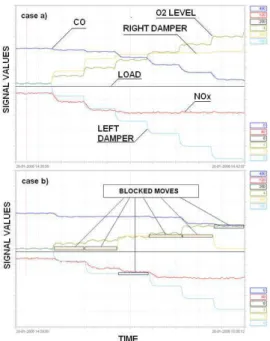
Figure 3: a) Example of control trajectory when: a) blocking algorithm is disabled, b) blocking algorithm is activated in each optimization step.
Figure 3a presents a simulation in which control vari-ables representing an oxygen level (O2 LEVEL) and a position of left damper (DAMPER LEFT) are correlated. It can lead to a situation when the matrixW is singular. Figure 3b presents, that a blocking algorithm is able to eliminate a linear dependence between mentioned signals. However, it results in worst quality of the solution. It is shown that one of minimized outputs (CO emission) has reached higher level in comparison to a situation when a blocking algorithm was turned off. Temporary accep-tance of suboptimal solution is needed, to provide a good conditioning of equation (3).
In addition to the presented methods, a heuristic applied in a stochastic optimization layer [4], eliminates potential linear dependences between columns of matrix ∆XL as
well as ∆XG. In this heuristic only one randomly chosen
control variable is changing at a time.
4
Results
SILO has been implemented in six units in U.S. power plants, four units in Polish power plants and one unit in Taiwan power plant. Results of a SILO implementa-tion in one of units in Polish power plants is presented in this chapter. The primary SILO goal was to keep NOx(nitrogen oxides) emission (one hour average) below
500 mg/Nm3 and keep CO (carbon monoxide) emission
(5 minute average) below 250 mg/Nm3. The secondary
SILO goal was to keep LOI (loss of ignition) below 5 %, keep SH (super heat) temperature on 540 ◦C and keep
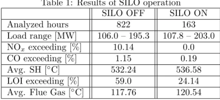
desulphur-Table 1: Results of SILO operation SILO OFF SILO ON Analyzed hours 822 163 Load range [MW] 106.0 – 195.3 107.8 – 203.0 NOx exceeding [%] 10.14 0.0
CO exceeding [%] 1.15 0.19 Avg. SH [◦C] 532.24 536.58
LOI exceeding [%] 59.0 24.14 Avg. Flue Gas [◦C] 117.76 120.54
ization process requirement).
SILO optimized nine output signals: CO emission (left and right side), NOx emission (left and right side),
es-timated SH temperature (left and right side), flue gas temperature (left and right side) and LOI signal. Six dis-turbance signals were chosen from the set of all process’s signals: unit load, coal calorific value and status of each of four coal mills. Control vector consisted of eleven sig-nals: O2 level, eight secondary air dampers and two OFA dampers.
Figure 4 presents a situation, when SILO is disabled and compares it with the situation when SILO is en-abled. SILO essentially reduces NOxemission and
main-tains CO emission and LOI below defined limit. Table 1 presents one month summary of SILO operation results. One can see that NOx emission limit (500 mg/Nm3) has
not been exceeded even once, when SILO was enabled. When SILO was turned off, 10.41 % of analyzed one hour averages was above this limit. By 99.81 % of SILO operation time, CO emission has been kept below 250 mg/Nm3. When SILO was disabled CO emission limit
has been kept below 250 mg/Nm3 by 98.85 % of time.
SH temperature has been increased by 4.4◦C, so the
effi-ciency of the process was higher, when SILO was enabled. LOI was reduced to 3.92 % (from 5.16 % level). SILO has kept LOI below 5 % by 75.9 % of its operation time. In comparison, when SILO was disabled, LOI was below the limit only by 41 % of time. When SILO was enabled, Flue Gas Temperature was kept below 140◦C all the time, so
flue gas desulphurization process has not been disturbed.
Figure 4: SILO influence on NOx, CO and LOI signals.
5
Summary
This paper presents some drawbacks connected with MPC controllers. MPC approach was compared with SILO. Furthermore two new methods, which provide good conditioning of model identification task, were pre-sented. These methods cause that a steady-state pro-cess’s model created by SILO represents a real derivative of a static process characteristic. Moreover results from one of SILO implementations in Polish power plant were presented. They confirm high efficiency of presented so-lution in solving real technical problems.
References
[1] L. N. De Castro and F.J. Von Zuben. Artificial im-mune systems: Part i – basic theory and applica-tions. Technical Report RT DCA 01/99, Department of Computer Engineering and Industrial Automation, School of Electrical and Computer Engineering, State University of Campinas, Campinas, SP, Brazil, De-cember 1999.
[2] L. Desborough and R. Miller. Increasing customer value of industrial control performance monitoring -honeywell’s experience. In Proc. of 2004 American Control Conference, Boston, USA, June 2004. [3] Piotr Tatjewski. Advanced Control of Industrial
Pro-cesses : Structures and Aglorithms. Springer Verlag, London, 2007.
[4] K. Wojdan and K. Swirski. Immune inspired opti-mizer of combustion process in power boiler. InProc. of the 20th International Conference on Industrial, Engineering & Other Applications of Applied Intelli-gent Systems, Kyoto, Japan, June 2007.
[5] K. Wojdan, K. Swirski, M. Warchol, and T. Cho-miak. New improvements of immune inspired opti-mizer SILO. InProc. of the 19th IEEE International Conference on Tools with Artificial Intelligence, Pa-tras, Greece, October 2007.