Controlled meteorological (CMET) balloon profiling of the Arctic atmospheric boundary layer around Spitsbergen compared to a mesoscale model

(1)

ACPD

15, 27539–27573, 2015

CMET balloon profiling of Arctic

ABL

T. J. Roberts et al.

Title Page

Abstract Introduction

Conclusions References

Tables Figures

◭ ◮

Back Close

Full Screen / Esc

Printer-friendly Version Interactive Discussion

Discussion

P

a

per

|

Discussion

P

a

per

|

Discussion

P

a

per

|

Discussion

P

a

per

|

Atmos. Chem. Phys. Discuss., 15, 27539–27573, 2015 www.atmos-chem-phys-discuss.net/15/27539/2015/ doi:10.5194/acpd-15-27539-2015

This discussion paper is/has been under review for the journal Atmospheric Chemistry and Physics (ACP). Please refer to the corresponding final paper in ACP if available.

Controlled meteorological (CMET) balloon

profiling of the Arctic atmospheric

boundary layer around Spitsbergen

compared to a mesoscale model

T. J. Roberts1,2, M. Dütsch3,4, L. R. Hole3, and P. B. Voss5

1

LPC2E/CNRS, 3A, Avenue de la Recherche Scientifique, 45071 Orléans, CEDEX 2, France

2

Norwegian Polar Institute, Fram Centre, 9296 Tromsø, Norway

3

Norwegian Meteorological Institute, Bergen, Norway

4

ETH Zürich, Switzerland

5

Smith College, Picker Engineering Program, Northampton MA, USA

Received: 22 May 2015 – Accepted: 12 September 2015 – Published: 14 October 2015

Correspondence to: T. J. Roberts (tjardaroberts@gmail.com)

(2)

ACPD

15, 27539–27573, 2015

ABL

Title Page

Tables Figures

◭ ◮

Back Close

Full Screen / Esc

Discussion

P

a

per

|

Discussion

P

a

per

|

Discussion

P

a

per

|

Discussion

P

a

per

|

Abstract

Observations from CMET (Controlled Meteorological) balloons are analyzed in com-bination with mesoscale model simulations to provide insights into tropospheric mete-orological conditions (temperature, humidity, wind-speed) around Svalbard, European High Arctic. Five Controlled Meteorological (CMET) balloons were launched from

Ny-5

Ålesund in Svalbard over 5–12 May 2011, and measured vertical atmospheric profiles above Spitsbergen Island and over coastal areas to both the east and west. One no-table CMET flight achieved a suite of 18 continuous soundings that probed the Arctic marine boundary layer over a period of more than 10 h. The CMET profiles are com-pared to simulations using the Weather Research and Forecasting (WRF) model using

10

nested grids and three di_fferent boundary layer schemes. Variability between the three model schemes was typically smaller than the discrepancies between the model runs and the observations. Over Spitsbergen, the CMET flights identified temperature in-versions and low-level jets (LLJ) that were not captured by the model. Nevertheless, the model largely reproduced time-series obtained from the Ny-Ålesund meteorological

15

station, with exception of surface winds during the LLJ. Over sea-ice east of Svalbard the model underestimated potential temperature and overestimated wind-speed com-pared to the CMET observations. This is most likely due to the full sea-ice coverage assumed by the model, and consequent underestimation of ocean–atmosphere ex-change in the presence of leads or fractional coverage. The suite of continuous CMET

20

soundings over a sea-ice free region to the northwest of Svalbard are analysed spa-tially and temporally, and compared to the model. The observed along-flight daytime increase in relative humidity is interpreted in terms of the diurnal cycle, and in the context of marine and terrestrial air-mass influences. Analysis of the balloon trajectory during the CMET soundings identifies strong wind-shear, with a low-level channeled

25

(3)

ACPD

15, 27539–27573, 2015

ABL

Title Page

Tables Figures

◭ ◮

Back Close

Full Screen / Esc

Discussion

P

a

per

|

Discussion

P

a

per

|

Discussion

P

a

per

|

Discussion

P

a

per

|

and boundary layer in remote regions where few other observations are available for model validation.

1 Introduction

The polar regions provide a challenge to atmospheric numerical models. Firstly, model parameterisations are often adapted to and validated against lower latitudes and might

5

not necessarily be applicable to high latitude processes. Secondly, there exists lim-ited detailed in-situ observational data for model initialization and validation in remote polar regions. Accurate representation polar meteorology and small-scale processes, is, however, essential for meteorological forecast models, whose comparison to ob-servations is particularly relevant for improving understanding of climate in the Arctic,

10

a region undergoing rapid change (Vihma, 2014). A particular challenge is that the po-lar atmospheric boundary layer (ABL) is usually strongly stable during winter, and only weakly stable to neutral during summer (Persson et al., 2002). This stability acts to magnify the e_ffects of flows over small scale topography, such as channeling, katabatic flows and mountain waves, and can promote the formation of low-level jets. Further, in

15

coastal areas, thermodynamic ice formation, growth and melt, and wind- and oceanic current driven advection of sea ice can lead to highly variable surface conditions that control air–sea exchange of heat and momentum, and affect the radiative balance e.g. through albedo. Snow layers deposited upon sea-ice provide a further insulating layer that modifies heat exchange between the ocean and the overlying atmosphere. For

20

example, for polar winter conditions at low atmospheric temperature (e.g.−40◦C), the

surface temperature of open water areas is practically at the freezing point of water (−1.8◦C), while the surface temperature of thick snow covered sea ice is substantially

lower, being close to the atmospheric temperature (e.g.−40◦C). Hence, the heat and

energy fluxes can vary by up to two orders of magnitude, depending on the surface

25

(4)

ACPD

15, 27539–27573, 2015

ABL

Title Page

Tables Figures

◭ ◮

Back Close

Full Screen / Esc

Discussion

P

a

per

|

Discussion

P

a

per

|

Discussion

P

a

per

|

Discussion

P

a

per

|

Thus, significant uncertainties remain in modelling Arctic meteorological variables. For example, a comparison of eight di_fferent RCM (Regional Climate Model) simula-tions over the Western Arctic to European Center for Medium–Range Weather Fore-cast (ECMWF) analyses over September 1997–September 1998 found general agree-ment to the model ensemble mean but large across-model variability, particularly in

5

the lowest model levels (Rinke et al., 2006). Direct comparisons of Arctic ABL mete-orology observations to mesoscale model simulations using the regional Weather Re-search and Forecasting (WRF) model (in standard or “polar” version) have also been performed. These include comparison to automatic weather stations (AWS) on the Greenland ice sheet in June 2001 and December 2002 (Hines and Bromwich, 2008);

10

to drifting ice station SHEBA meteorological measurements over the Arctic Ocean in 1997–1998 (Bromwich et al., 2009); to tower observations and radio-sonde soundings in three Svalbard (Spistbergen) fjords in winter and spring 2008 (Kilpeläinen et al., 2011); to AWS stations along Kongsfjorden in Svalbard in spring 2010 (Livik, 2011); to meteorological mast measurements in Wahlenbergfjorden, Svalbard in May 2006

15

and April 2007 (Makiranta et al., 2011); to tethered balloon soundings and mast ob-servations in Advent- and Kongsfjorden in Svalbard in March-April 2009 (Kilpeläinen et al., 2012), and to a remotely controlled model aircraft equipped with meteorological sensors (the small unmanned meteorological observer, SUMO) over Iceland and Ad-vent valley in Svalbard (Mayer et al., 2012a, b). These studies collectively found that

20

(Polar) WRF was able to partially reproduce the meteorological observations, typically only when operated at higher model resolution (e.g. 1 km). Sea-ice was found to be particularly important at high sea–air temperature di_fferences, and occurrence of low-level jets were observed yet not always reproduced by the model. Such comparisons between model and observations are, however, limited by the spatial scale of the field

25

observations, typically only a few km.

(5)

ACPD

15, 27539–27573, 2015

ABL

Title Page

Tables Figures

◭ ◮

Back Close

Full Screen / Esc

Discussion

P

a

per

|

Discussion

P

a

per

|

Discussion

P

a

per

|

Discussion

P

a

per

|

within the troposphere at designated altitudes, and can take vertical soundings at any time during the balloon flight on commanded via satellite link (Voss et al., 2013). The CMETs can also be configured for automated profiling of the atmospheric boundary layer during the flight, as we demonstrate in this study. The nested dual balloon design ensures very little helium loss, enabling the balloons to make multi-day flights. This

5

gives the opportunity to investigate areas far away from research bases, at greater spatial scales (many hundreds of kilometers from the launch point) than can be ob-tained by line-of-sight unmanned aerial vehicle (UAV) approaches, radio-sondes or tethered balloons. Previous CMET balloon applications include Riddle et al. (2006), Voss et al. (2010), Mentzoni (2011) and Stenmark et al. (2014). Voss et al. (2010)

in-10

vestigated the evolving vertical structure of the polluted Mexico City Area outflow by making repeated balloon profile measurements of temperature, humidity and wind in the advecting outflow. Riddle et al. (2006) and Mentzoni (2011) used the CMET bal-loons as a tool to verify atmospheric trajectory models – namely FlexTra (Stohl et al., 1995) and FlexPart (Stohl et al., 1998) – in the United States and in the Arctic,

respec-15

tively. Stenmark et al. (2014) combined data from CMETs, ground-based and a small model airplane data with WRF simulations to highlight the role of nunatak-induced con-vection in Antarctica.

Here we compare the soundings performed during the five Svalbard balloon flights of May 2011 to simulations made using the Weather Research and Forecasting (WRF)

20

mesoscale model with three di_fferent boundary layer schemes, and thereby provide insights into key processes influencing meteorology of remote Arctic regions.

2 Methods

2.1 Observations

Five CMET balloons were launched from the research station of the Alfred Wegener

25

(6)

ACPD

15, 27539–27573, 2015

ABL

Title Page

Tables Figures

◭ ◮

Back Close

Full Screen / Esc

Discussion

P

a

per

|

Discussion

P

a

per

|

Discussion

P

a

per

|

Discussion

P

a

per

|

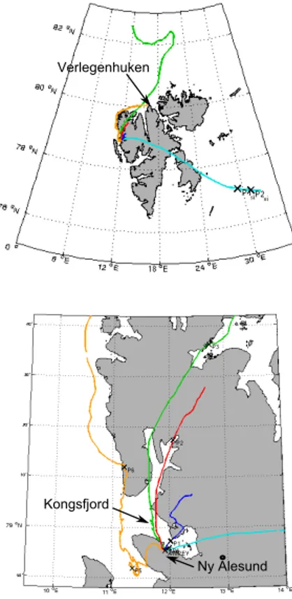
period 5 to 12 May 2011. The CMET payload included meteorological sensors for tem-perature, relative humidity (RH) and pressure, as well as GPS and satellite modem for in-flight control. The CMET balloon design and control algorithms are described in detail by Voss et al. (2013). Figure 1a and b shows the balloon flights of the May 2011 campaign as well as two meteorological sites providing additional ground-based data:

5

the Ny-Ålesund AWI-PEV station (from where the balloons were launched), and Ver-legenhuken in North-East Spitzbergen. Balloons 1 and 2 had short flights due to tech-nical issues encountered at the start of the campaign, and included only one vertical sounding each. Balloon 3 flew far north but did not perform soundings after leaving the coastal area of Spitzbergen, thus only the vertical sounding (ascent and descent) at

10

the very beginning of the flight is used for this study. Balloon 4 flew eastwards, but de-spite strong balloon performance needed to be terminated before encroaching Russian airspace. In addition to its vertical sounding obtained shortly after launch it includes two closely spaced (ascent and descent) soundings over sea-ice east of Svalbard. Balloon 5 undertook a 24 h duration flight that first exited Kongsfjorden, then flew northwards

15

along the coast and measured a much longer series of 18 consecutive profiles of the ABL in automatic sounding mode, before being raised to higher altitudes where winds advected it eastwards (Voss et al., 2013). To the best of our knowledge, this was the first automated sounding sequence made by a free balloon.

Temperature and humidity profiles were extracted from the CMET flights for model

20

comparison as indicated in Fig. 1a and b, in locations over Svalbard topography, over a sea-ice covered region east of Svalbard, and over a sea-ice free region west of Sval-bard where continuous automated soundings were performed. The capacitance humid-ity sensor (G-TUCN.34 from UPSI, covering 2 to 98 % RH range over−40 to+85◦C)

generates a signal which is a function of the ambient relative humidity (RH) with

re-25

(7)

ice-ACPD

15, 27539–27573, 2015

ABL

Title Page

Tables Figures

◭ ◮

Back Close

Full Screen / Esc

Discussion

P

a

per

|

Discussion

P

a

per

|

Discussion

P

a

per

|

Discussion

P

a

per

|

free ocean west of Svalbard). Where present, they could promote ice deposition, thus act to lower the water saturation vapour pressure. In such conditions, RH calculated over water underestimates the RH with respect to ice. Nevertheless, for the relatively warm ambient surface temperatures encountered over ice during the campaign (typ-ically a few degrees negative◦

C or higher) such e_ffects are modest. For consistency,

5

RH over water is reported across the field-campaign and is similarly illustrated for the model output.

For comparison to two WRF nested model runs (see details below), the balloon profiles were interpolated to 50 m height intervals and the measurement from paired ascent/descent soundings were averaged at each height. These ascent/descent

pro-10

files typically each required between 30 min and about one hour depending on the al-titude change. These averaged ascent/descent profiles were compared to WRF model output at the longitude and latitude of the balloon location at the maximum of its as-cent/descent cycle, averaged over a full hour centred on the middle of the balloon profile. A more detailed analysis was made of the meteorological evolution observed

15

during consecutive automated soundings of flight 5, by comparing to WRF output at selected times along a transect line approximately following the CMET flight path, and geographically within the model layer corresponding to the average CMET flight alti-tude.

2.2 Numerical model implementation

20

Regional model simulations were performed using the Weather Research and Fore-cast (WRF) version 3.3.1. It is based on non-hydrostatic and fully compressible Euler equations that are integrated along terrain-following hydrostatic-pressure (sigma) coor-dinates, see Skamarock et al. (2008). The model was run for the simulation period from 3 May 2011, 00:00 UTC to 12 May 2011, 00:00 UTC allowing for a spin up time of 48 h.

25

(8)

loca-ACPD

15, 27539–27573, 2015

ABL

Title Page

Tables Figures

◭ ◮

Back Close

Full Screen / Esc

Discussion

P

a

per

|

Discussion

P

a

per

|

Discussion

P

a

per

|

Discussion

P

a

per

|

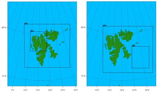
tions are shown in Fig. 2. The outer domain was centered at 78.9◦

N, 16.5◦

E (78.9◦

N, 19.5◦

E for model run 2) and included 114×94 gridpoints covering the whole Svalbard

archipelago and a large part of the surrounding Arctic ocean. The second domain in-cluded 175×184 (187×202) gridpoints for model run 1 (model run 2) and covered

the whole Svalbard archipelago, whilst the innermost domain, which covered the area

5

where the correspondent balloon profiles and timeseries were measured, had 232×190

(253×202) gridpoints for model run 1 (model run 2). All three domains had a high

ver-tical resolution with 61 terrain-following sigma levels, where the model top was set to 50 hPa. The lowest 1000 m included 19 model levels with the lowest full model level at 19 m. Static field data, such as topography and land use index, were provided by

10

the US Geological Survey in a horizontal resolution of 30 arcseconds (0.9 km in north– south direction). Initial and lateral boundary conditions were taken from the ECMWF operational analysis data on a 0.125◦

×0.125◦horizontal resolution and on 91 vertical

levels, and updated every six hours. Sea ice and sea surface temperature (SST) were taken directly from the ECMWF data at the time the simulation started (3 May 2011)

15

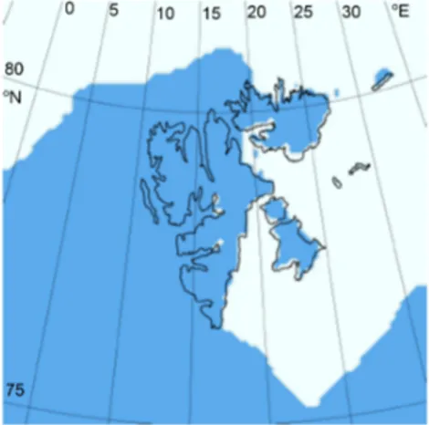
and remained fixed during the whole simulation period, assuming full sea-ice cover-age for any model grid-point with positive sea-ice flag. This approach is justified by the good agreement between the ECMWF sea-ice flag and satellite images of sea-ice coverage on 5 May, both showing dense sea-ice east of Svalbard (Fig. 3). Conversely, to the west of Svalbard, sea-ice is absent. Sea surface temperatures are, as usual,

20

higher to the west than east of Svalbard. This is due to the northward flowing warm and saline Atlantic Warm Current (AWC) or “Gulf stream” that elevates temperatures along Svalbard’s west coast (the AWC subsequently sinks below the cold polar waters further north).

For cloud microphysics the WRF single moment 3-class simple ice scheme

(Dud-25

(9)

ACPD

15, 27539–27573, 2015

ABL

Title Page

Tables Figures

◭ ◮

Back Close

Full Screen / Esc

Discussion

P

a

per

|

Discussion

P

a

per

|

Discussion

P

a

per

|

Discussion

P

a

per

|

cover prediction (Chen and Dudhia, 2001). In the first and second domain, the Kain– Fritsch cumulus scheme (Kain, 2004) was applied in addition, whereas in the third domain, cumulus convection was neglected.

Sensitivity tests were made with three different boundary layer parameterisation schemes as follows: the Yonsei University (YSU) scheme (Hong et al., 2006) is a

non-5

local first order closure scheme that uses a counter gradient term in the eddy diffusion equation, and is the default ABL scheme in WRF. The Mellor–Yamada–Janjic (MYJ) scheme (Janjic, 1990, 1996, 2002) uses the local 1.5 order (level 2.5) closure Mellor– Yamada model (Mellor and Yamada, 1982), where the eddy diffusion coefficient is de-termined from the prognostically calculated turbulent kinetic energy (TKE). According

10

to Mellor and Yamada (1982), it is an appropriate scheme for stable to slightly unstable flows, while errors might occur in the free convection limit. The Quasi-Normal Scale Elimination (QNSE) scheme (Sukoriansky et al., 2006) is, as the MYJ scheme, a local 1.5 order closure scheme. In contrast to the MYJ scheme, it includes scale dependence by using only partial averaging instead of scale independent Reynolds averaging, and

15

is therefore able to take into account the spatial anisotropy of turbulent flows. It is thus considered especially suited for the stable ABL.

3 Results and discussion

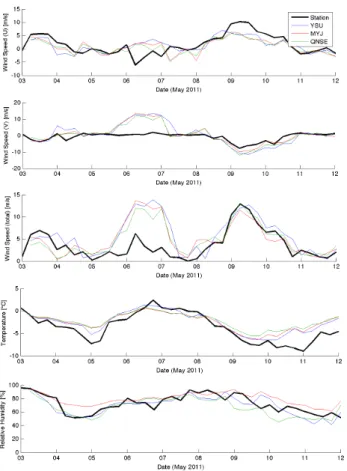
3.1 Meteorological conditions and ground-stations compared to the WRF

simulation

20

The period of 3–12 May 2011 was characterized by rapidly changing meteorological conditions, reflected in the di_fferent CMET flight paths (Fig. 1a and b) and the 6 hourly averaged meteorological station surface observations shown in Fig. 4 (AWIPEV, Ny-Ålesund) and Supplement S1 (Verlegenhuken, N Svalbard). At first, northerly winds carried cold air to Ny-Ålesund, causing surface temperatures to decline, reaching an

25

(10)

ACPD

15, 27539–27573, 2015

ABL

Title Page

Tables Figures

◭ ◮

Back Close

Full Screen / Esc

Discussion

P

a

per

|

Discussion

P

a

per

|

Discussion

P

a

per

|

Discussion

P

a

per

|

winds over not much more than one day, leading to increasing temperatures and an hourly maximum of 2.9◦

C on 6 May. The wind direction subsequently become more westerly and then northerly with high wind-speeds on 8 and 9 May, given occurrence of a high pressure system SW and a lower pressure system NE of Svalbard, and the AVI-PEV station registered a maximum wind-speed of 17.4 m s−1

around noon on 9 May.

5

This was followed by a period of lowwind-speed over 11–12 May, also reflected in the 24 h CMET flight to the east of Svalbard, with low temperatures recorded at the Spits-bergen meteorological stations. The WRF simulations show good general agreement to the 6 hourly averaged surface meteorological observations at Ny-Ålesund, Fig. 4, (and Verlegenhuken station in N Svalbard, Fig. S1 in the Supplement), with similar

re-10

sults for all three ABL schemes. However, the high (>10 m s−1) southerly surface winds

predicted on 6–7 May for Ny-Ålesund were not observed. Outside of these dates, the model generally reproduced the winds, albeit at a wind direction 30◦

greater (clockwise) than typically observed in Ny-Ålesund (see wind-roses, Fig. S2), likely due to a wind channeling e_ffect in the Kongsfjorden that is not fully captured by the model.

Temper-15

ature was well reproduced however somewhat overestimated during cold periods (e.g. 5 and 11–12 May) at both surface stations.

3.2 Atmospheric boundary layer over Spitsbergen: topography, inversions and

low level jets

The four CMET soundings over Svalbard topography are compared to WRF

wind-20

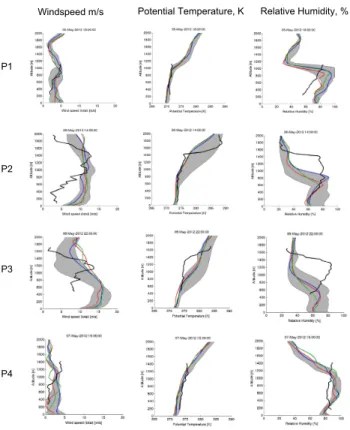
speed, relative humidity and temperature profiles in Fig. 5, for the three different bound-ary layer schemes. Notably the results using the three ABL schemes are not strongly di_ffering from each other, but collectively show greater disagreement to the observed ABL profiles. WRF captures the profiles with weak winds (profile 1, 4) well, but not on 5– 6 May (profile 2, 3) where the CMET observations show the occurrence of a weak low

25

(11)

ACPD

15, 27539–27573, 2015

ABL

Title Page

Tables Figures

◭ ◮

Back Close

Full Screen / Esc

Discussion

P

a

per

|

Discussion

P

a

per

|

Discussion

P

a

per

|

Discussion

P

a

per

|

to predict the lofted altitude of the LLJ appears connected to the model overestimation of surface wind-speed in Ny-Ålesund on 5–6 May (a model-observation discrepancy not found in Verlegenhuken further north in Svalbard). The occurrence of LLJs is likely promoted by the Svalbard topography in conjunction with a stable boundary layer.

These model-observation discrepancies are consistent with previous studies:

Mold-5

ers and Kramm (2010) found that WRF had difficulties in capturing the full strength of the surface temperature inversion observed during a five day cold weather period in Alaska. Kilpeläinen et al. (2012) found that WRF reproduced only half the observed inversions, and often underestimated their depth and strength, and that the average modeled LLJ was deeper and stronger than that observed. An overestimation of

sur-10

face wind-speeds by WRF, especially in case of strong winds, has also been reported by Claremar et al. (2012), in comparison to AWS placed on three Svalbard glaciers, and by Kilpeläinen et al. (2011) and Kilpeläinen et al. (2012), in a study of Kongsfjorden. Since low wind-speeds are associated with inversion formation, WRF’s overestimation of wind-speed might partly explain the di_fficulties in capturing (the strength of)

inver-15

sions (Molders and Kramm, 2010). Consequently, since elevated inversions are often connected to low level jets (Andreas et al., 2000), the di_fficulties in capturing inversions could help explain the model di_fficulties in predicting low level jets.

A likely limitation to the WRF model capability over complex topography is its hori-zontal and vertical resolution. The model set-up used here includes 61 vertical layers,

20

which Mayer et al. (2012b) suggests are necessary to resolve ABL phenomena, such as low level jets. However, Esau and Repina (2012) note that even a model resolution of 1 km in the horizontal does not properly represent the valley and steep surrounding mountains in Kongsfjorden, finding that even a fine resolution model (56×61 m grid cell,

20 times higher than the 1 km grid cell used in this and other WRF studies) could not

25

(12)

ACPD

15, 27539–27573, 2015

ABL

Title Page

Tables Figures

◭ ◮

Back Close

Full Screen / Esc

Discussion

P

a

per

|

Discussion

P

a

per

|

Discussion

P

a

per

|

Discussion

P

a

per

|

3.3 CMET atmospheric profiles east of Spitsbergen: the role of sea-ice

The two consecutive CMET profiles over sea-ice east of Svalbard are compared to WRF model run 2 in Fig. 6. All three schemes tend to overestimate wind-speed, es-pecially at the low levels. Nevertheless the slope of the wind profile corresponds ap-proximately to the observations. Potential temperature is underestimated by around

5

2.5 K in all schemes. The largest difference between the observations and the model is found at the low levels, where it reaches up to 4 K. However, relative humidity is in better agreement, meaning that specific humidity must also be lower in the model than in the observations (e.g. a 4 K difference at 85 % RH corresponds to a 9×10−4kg m−3

absolute humidity, a difference of around one quarter to one third ambient levels). The

10

temperature and specific humidity bias is most probably due to an over representation of sea ice in the WRF model setup, which exerts a strong control on surface condi-tions. Even though the sea ice flag from the ECMWF data seems to agree fairly well with satellite sea-ice observations (Fig. 3), areas of polynyas and leads that can be recognized on the satellite picture were represented as homogeneous sea ice in the

15

model. Further, the 100 % sea-ice coverage assumed in the model for grid cells with positive sea-ice flag may not reflect reality: small patches of open water amongst very close (90–100 %) or close (80–90 %) drift ice would promote sea–air exchange, en-hancing both temperature and specific humidity at the surface (Andreas et al., 2002).

Inclusion of fractional sea-ice in WRF (available for WRF version 3.1.1 and higher)

20

might rectify this problem, but is not straightforward to implement: the amount of sea ice in a grid cell varies with time through sea ice formation, break up and drifting, the latter typically a dominant control on ice-presence during late spring east of Svalbard. However, the WRF meteorological model does not simulate surface oceanographic processes, thus predicted sea-ice presence depended only on whether the SST was

25

(13)

ACPD

15, 27539–27573, 2015

ABL

Title Page

Tables Figures

◭ ◮

Back Close

Full Screen / Esc

Discussion

P

a

per

|

Discussion

P

a

per

|

Discussion

P

a

per

|

Discussion

P

a

per

|

as in Kilpeläinen et al. (2012), but this becomes demanding over large regions. Nev-ertheless, given its strong control on ABL processes, a fractional sea-ice approach is recommended for future studies, particularly if a longer series of CMET soundings can be achieved, e.g. during balloon flights advected in a pole-ward direction, rather than towards Russia, which necessitated the flight to be terminated on command after only

5

two profiles in our study.

3.4 Automated CMET soundings during a 24 h flight west of Spitsbergen

Flight 5 provided a series of 18 boundary-layer profiles over a largely sea-ice free re-gion west of Svalbard. With the low wind-speeds (<5 m s−1), the 24 h balloon trajectory

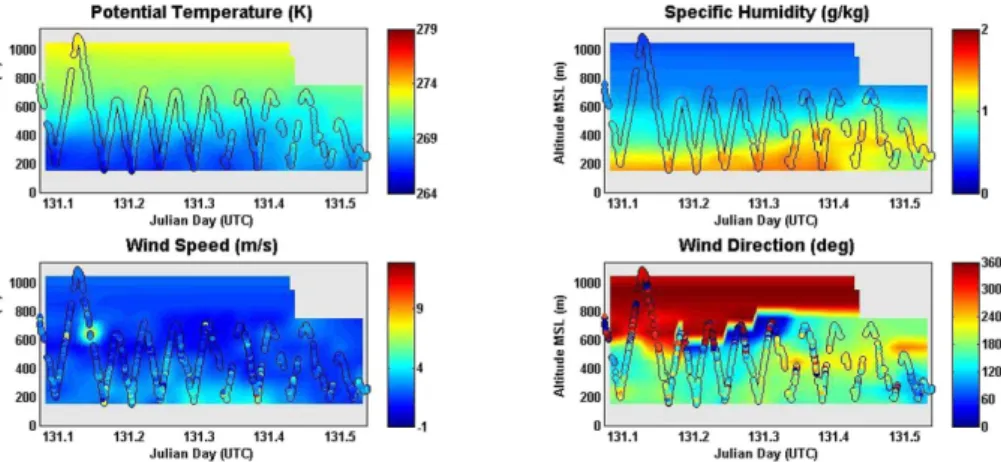
remained relatively close to Svalbard coastline. Figure 7 shows the observed profiles

10

of potential temperature, specific humidity, wind-speed and wind-direction, with inter-polated data between the soundings. The soundings ranged from approximately 150 to 700 m during the first part of the flight (∼02:00–12:30 UTC, JD 131.08–131.52).

Specific humidity is greatest and potential temperature lowest nearer the surface, as expected. Specific humidity tends to increase during the flight, particularly in the lower

15

and middle levels, which can be interpreted as a diurnal enhancement from surface evaporation. However, beyond JD 131.40 (09:36 UTC) there is actually a decrease in humidity in the lowermost levels, with maximum humidity in the sounding occurring around 350 m. Concurrent to this there is also a small increase in potential temperature at low altitudes. The wind-speed and direction plots indicate relatively calm conditions,

20

with greatest wind-speed in the lower levels generally from a southerly direction. In contrast, at the top of the soundings the balloon encountered winds from a northerly direction, above 600 m. From JD 131.35 onwards, the observed winds became broadly southerly also at 600 m. However, a band of rather more west-south-westerly winds de-veloped at mid-altitudes (∼450 m), and low-level winds became (east)-south-easterly

25

(14)

ACPD

15, 27539–27573, 2015

ABL

Title Page

Tables Figures

◭ ◮

Back Close

Full Screen / Esc

Discussion

P

a

per

|

Discussion

P

a

per

|

Discussion

P

a

per

|

Discussion

P

a

per

|

While the complex flow in this case largely precludes a quasi-Lagrangian-type process study, the series of profiles none-the-less provides a nuanced understanding that is not possible with traditional rawinsondes or constant-altitude balloons.

The CMET observations appear consistent with the occurrence of a low-level flow that is decoupled from higher altitudes, and – at least initially – a diurnal increase

5

in surface humidity through enhanced ocean evaporation. The observed wind-shear is consistent with a tilted high pressure system (that tilts with altitude towards the west of Svalbard, according to the WRF model), whilst surface winds may be fur-ther influenced by low-level channel flows. An outflow commonly exits from nearby Kongsfjorden-Kongsvegen valley (e.g. Esau and Repina, 2012) but is hard to identify

10

from the ground-station in Ny Ålesund (south side of Kongsfjorden) given the rather low wind-speeds during this period. Winds that originate over land are likely colder, with lower humidity than marine air masses. Thus, the CMET observations of lower specific humidity between JD 131.40–131.5 (09:36–12:00 UTC) might be explained by fumigation from or simply sampling of such a channel outflow. Alternatively, the CMET’s

15

location over Kapp Mitra Penninsula at this time may indicate an even more local source of dry air impacting low levels. A final possibility could be overturning of air masses in the vertical, bringing less humid air, with higher potential temperature to lower altitudes. At mid-levels (∼450 m) a relatively humid air layer persists, properties which suggest it

likely has origins from the surface. It appears to be advected north-eastwards,

poten-20

tially replenishing air over Svalbard to replace that which may be lost from the channel outflow. Further discussion is provided in conjunction with the WRF model results.

The CMET observations are compared to WRF model output at two time-periods, 07:00 and 15:00 UTC on 11 May (JD 131.3 and 131.6, respectively). Model output (in 2-D) is presented in two ways: (i) cross-sections of relative humidity (RH) and potential

25

temperature with altitude along a transect in the WRF model (QNSE, YSU and MYJ schemes) that lies in an approximately S–N direction and is reasonably close to (but not identical to) the balloon flight path, see Fig. 8, (ii) maps of temperature and abso-lute humidity (kg kg−1

(15)

ACPD

15, 27539–27573, 2015

ABL

Title Page

Tables Figures

◭ ◮

Back Close

Full Screen / Esc

Discussion

P

a

per

|

Discussion

P

a

per

|

Discussion

P

a

per

|

Discussion

P

a

per

|

oceans although reaching higher altitudes over the Svalbard terrain) that provide a geo-graphic spatial context. For clarity, only output from WRF MYJ BL scheme is illustrated (see Supplement for QNSE and YSU schemes).

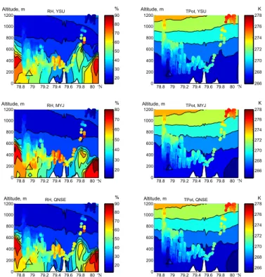
For (i), the WRF model temperature and humidity cross-sections at 07:00 and 15:00 UTC are shown alongside CMET observations along the whole balloon flight, in

5

Figs. 9 and 10, respectively, and where the balloon locations at 07:00 and 15:00 UTC are denoted by a triangle or cross, respectively. The model generally agrees with the balloon observations: potential temperature increases with altitude, and surface tem-perature decreases with increasing latitude in the 07:00 UTC cross-section. Bound-ary layer height is denoted by a sharp humidity decrease, at approx. 600 m (declining

10

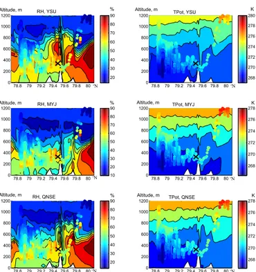
to 400 m at higher latitudes) in the 07:00 UTC WRF cross-section. For all the model schemes, a greater relative humidity and a higher boundary layer is predicted in the 15:00 UTC cross-section, as expected from the diurnal cycle, whereby solar heating increases evaporation to enhance RH, and increases thermal buoyancy to enhance ABL height. By 15:00 UTC, the model potential temperature is also generally higher,

15

however, surface temperatures now increases with latitude. This may reflect greater solar heating experienced at higher Arctic latitudes in the spring.

This overall RH trend of the model is in agreement to the observations: the CMET balloon data also exhibits a higher relative humidity at 15:00 UTC than 07:00 UTC. There is also some variability between the di_fferent model boundary layer schemes:

20

for the 15:00 UTC cross-section boundary layer height, YSU>QNSE>MYJ in terms of

both relative humidity and ABL height. However, diurnal variability is not the only control on ABL humidity (as discussed above). The geographical influence is illustrated by (ii); spatial maps of absolute humidity across a model layer (corresponding to∼300 m a.s.l.

over oceans, somewhat higher over land) in Fig. 11. As expected, humidity in the

ma-25

(16)

ACPD

15, 27539–27573, 2015

ABL

Title Page

Tables Figures

◭ ◮

Back Close

Full Screen / Esc

Discussion

P

a

per

|

Discussion

P

a

per

|

Discussion

P

a

per

|

Discussion

P

a

per

|

above. The model results presented at 07:00 UTC and 15:00 UTC clarify this influence in a geographic context. Between launch and 07:00 a.m. UTC the CMET moved into a more marine environment thus humidity increased. The balloon then moved north-wards, perhaps drawn by a channel outflow from Kingsbay. Over this period humidity is constant or declining slightly, as the balloon passes across Kongsfjorden Bay and

5

over the Kapp Mitra peninsula. From ∼midday to 15:00 UTC the humidity increases

again as the balloon travels northwards (a temporary westerly diversion occurs fol-lowing blocking of the low-level flow by Svalbard terrain). This humidity enhancement appears mostly caused by the diurnal effects of enhanced evaporation. Alternatively, simple transport of the balloon into or air-mass mixing with moister marine air could

10

play a role, but in any case the diurnal humidity signal appears strong across this NW region. After 15:00 UTC the balloon was raised to higher altitudes hence the humidity decreased compared to that in the fixed model level (a similar decrease can be seen in the model altitude-transect plots, Fig. 10).

Finally, we return to the subject of the quasi-Lagrangian nature of the CMET

bal-15

loon flight. A detailed analysis is beyond the scope of this study, nevertheless the wind, humidity and temperature observations indicate presence of more than one air mass in this coastal region. Whilst CMETs have previously been used in Lagrangian-type experiments to track the evolution of an airmass (e.g., Voss et al., 2010), this case-study presents more complex atmospheric conditions. Both vertical winds and

hori-20

zontal wind-shear can a_ffect the Lagrangian nature of the CMET balloon experiment. Vertical air mass movement is not measured by the CMET payload but is estimated by the WRF model to be su_fficiently low (typically≪0.01 m s−1) to be negligible in

most cases, with the exception of localized areas in QNSE scheme (see Supplement, Fig. S4). The CMET balloon movement was itself used to determine horizontal winds

25

(17)

tech-ACPD

15, 27539–27573, 2015

ABL

Title Page

Tables Figures

◭ ◮

Back Close

Full Screen / Esc

Discussion

P

a

per

|

Discussion

P

a

per

|

Discussion

P

a

per

|

Discussion

P

a

per

|

nique assumes horizontally uniform flow (in the vicinity of the balloon and computed trajectories) during the 8 h period starting in the early morning of 11 May, Fig. 12. The lowermost layer exhibited greatest wind-speed thus has the longest (and least certain) trajectory, approximately double that of the balloon during the same period. The upper-most layer flows southwards before reversing direction, approximately returning to its

5

initial position. The middle layer trajectory is quite similar to that of the CMET balloon, but is transported initially somewhat more westwards, and later somewhat more east-wards, due to the ESE winds experienced in the late morning (see Fig. 7). It is worth noting this final direction mirrors findings from two of the other CMET flights, whose initial paths out of Kongsfjorden deviated to the north-east into nearby Krossfjorden.

10

While the balloon-based trajectories and repeating profile measurements are not La-grangian, they do provide insight into the complex dynamics of low-altitude circulation influenced by complex terrain. Furthermore, the trajectories and profile data can be computed and displayed in near-real time, allowing future experiments to be modified during flight (e.g., to track specific layers or events). Such experiments can provide

15

observational insights that help constrain the complex meteorology.

4 Conclusions

Five Controlled Meteorological (CMET) balloons were launched from Ny-Ålesund, Svalbard on 5–12 May 2011, to measure the meteorological conditions (RH, tempera-ture, wind-speed) over Spitsbergen and in the surrounding Arctic region. Analysis of the

20

meteorological data, in conjunction with simulations using the Weather and Research Forecasting (WRF) model at high (1 km) resolution provide insight into processes gov-erning the Arctic atmospheric boundary layer and its evolution.

Three ABL parameterizations were investigated within the WRF model, YSU (Yon-sei University), MYJ (Mellor–Yamada–Janjic) and QNSE (Quasi-Normal Scale

Elimina-25

(18)

ACPD

15, 27539–27573, 2015

ABL

Title Page

Tables Figures

◭ ◮

Back Close

Full Screen / Esc

Discussion

P

a

per

|

Discussion

P

a

per

|

Discussion

P

a

per

|

Discussion

P

a

per

|

modelling in the Arctic, as identified from this study to include (i) the occurrence of inver-sions and low level jets over Svalbard topography in association with stable boundary conditions, which likely can only be captured at greater model resolution (ii) the pres-ence of (fractional) sea-ice that acts to modify sea–air exchange, but whose dynamical representation in the model is not straight-forward to implement.

5

The WRF model simulations showed good general agreement to surface meteoro-logical parameters (temperature, wind-speed, RH) in Ny Ålesund and Verlegenhuken, N Svalbard over 3–12 May 2011. However, temperatures were somewhat underesti-mated during colder periods, and surface winds were severely overestiunderesti-mated on 5–6 May in Ny Ålesund. Comparison of four CMET profiles over Svalbard topography to

10

the WRF model indicated model di_fficulties in capturing inversion layers and a low-level jet (LLJ). The CMET observations thereby provided a context for the predicted high surface wind-speeds in Ny Ålesund, which were observed aloft but not at the surface during the campaign. A higher resolution is likely required to improve the model ability to simulate the small-scale atmospheric dynamics particularly for stable Arctic

bound-15

ary layer conditions combined with Svalbard topography.

Two CMET soundings also probed the boundary layer over sea-ice to the east of Svalbard, during a balloon flight which despite good performance needed to be ter-minated to avoid encroaching on Russian territory. Model biases in wind-speed and surface level temperature (and inferred for specific humidity) over this region are likely

20

due to the representation of ice in the model. Whilst the ECMWF-derived sea-ice flag used appears reasonable, the presence of fractional sea-sea-ice east of Svalbard may have enabled greater air–sea exchange of heat and moisture than predicted by the model, which assumed 100 % sea-ice coverage for positive sea-ice flag. Fractional rep-resentation of sea-ice in WRF is thus desirable, but is not straightforward to implement

25

(19)

sea-ACPD

15, 27539–27573, 2015

ABL

Title Page

Tables Figures

◭ ◮

Back Close

Full Screen / Esc

Discussion

P

a

per

|

Discussion

P

a

per

|

Discussion

P

a

per

|

Discussion

P

a

per

|

ice during longer duration CMET flights (i.e. northerly rather than easterly advected) can be achieved.

A series of continuous automated soundings was performed during a CMET flight over a sea-ice free region west of Svalbard, tracing atmospheric boundary layer tem-perature and relative humidity profiles along the flight and with altitude. Meteorological

5

conditions encountered were complex, including a low-level flow decoupled from the air mass at higher altitudes. An increase in low-level relative humidity was observed, consistent with diurnal enhancement expected from evaporation. The WRF model pre-dicted both an increase in RH and ABL height over the diurnal cycle concurrent with the CMET observations. The data-model interpretation also considers influence of air

10

masses of di_fferent origin which augment the diurnal trends: air masses originating over the warm saline ocean waters have typically greater humidity than over the cold Svalbard topography.

Finally, the semi-Lagrangian nature of CMET flights is discussed. In this ABL study the balloon likely sampled di_fferent air masses through vertical soundings undertaken

15

during the flight, under conditions of strong vertical wind-shear. Analysis of the ob-served wind-fields provides an indication of the balloon trajectory in the context of surrounding wind trajectories at di_fferent altitudes.

In summary, CMET balloons provide a novel technological means to profile the re-mote Arctic boundary layer over multi-day flights, including the capacity to perform

20

multiple automated soundings. CMET capabilities are thus highly complementary to other Arctic observational strategies including fixed station, free and tethered balloons, and UAVs. Whilst UAVs o_ffer full 3-D spatial control for obtaining the meteorological observations, their investigation zone is generally limited to tens of kilometers based on both range and regulatory restrictions. CMETs flights provide a relatively low-cost

25

(20)

ACPD

15, 27539–27573, 2015

ABL

Title Page

Tables Figures

◭ ◮

Back Close

Full Screen / Esc

Discussion

P

a

per

|

Discussion

P

a

per

|

Discussion

P

a

per

|

Discussion

P

a

per

|

processes that control the observed evolution of meteorological parameters and that pose a challenge to mesoscale simulations of the Arctic atmosphere.

The Supplement related to this article is available online at doi:10.5194/acpd-15-27539-2015-supplement.

Acknowledgements. This research was sponsored by the Research Council of Norway and

5

the Svalbard Science Forum. We are very grateful to the joint French–German Arctic Research Base AWIPEV in Ny-Ålesund for logistical support, and Anniken C. Mentzoni for fieldwork assis-tance. T. J. Roberts acknowledges NSINK, an Arctic Field Grant, CRAICC, and the VOLTAIRE LABEX (VOLatils-Terre Atmosphère Interactions – Ressources et Environnement) ANR-10-LABX-100-01 (2011–2020) for funding. P. B. Voss acknowledges Smith College for support.

10

This study occurred at the end of the Coordinated Investigation of the Climate–Cryosphere Interactions (CICCI) initiative.

References

Andreas, E. L., Claffey, K. J., and Makshtas, A. P.: Low-level atmospheric jets and inversions

over the western Weddell sea, Bound.-Lay. Meteorol., 97, 459–486, 2000.

15

Andreas, E. L., Guest, P. S., Persson, P. O. G., Fairall, C. W., Horst, T. W., Moritz, R. E., and Semmer, S. R.: Near-surface water vapor over polar sea ice is always near ice saturation, J. Geophys. Res.-Oceans, 107, 8033, doi:10.1029/2000JC000411, 2002.

Bromwich, D. H., Hines, K. M., and Bai, L.-S.: Development and testing of polar weather research and forecasting model: 2. Arctic Ocean., J. Geophys. Res., 114, D08122,

20

doi:10.1029/2008JD010300, 2009.

Chen, F. and Dudhia, J.: Coupling an advanced land-surface/hydrology model with the Penn State/NCAR MM5 modeling system. part i: Model description and implementation, Mon. Weather Rev., 129, 569–585, 2001.

Claremar, B., Obleitner, F., Reijmer, C., Pohjola, V., Waxeg, A., Karner, F., and

Rutgers-25

(21)

ACPD

15, 27539–27573, 2015

ABL

Title Page

Tables Figures

◭ ◮

Back Close

Full Screen / Esc

Discussion

P

a

per

|

Discussion

P

a

per

|

Discussion

P

a

per

|

Discussion

P

a

per

|

Dudhia, J.: Numerical study of convection observed during the winter monsoon experiment using a mesoscale two-dimensional model, J. Atmos. Sci., 46, 3077–3107, 1989.

Esau, I. and Repina, I.: Wind climate in Kongsfjorden, Svalbard, and attribution of leading wind driving mechanisms through turbulence-resolving simulations, Adv. Meteorol., 2012, 568454, doi:10.1155/2012/568454, 2012.

5

Hines, K. M. and Bromwich, D. H.: Development and testing of polar weather research and forecasting (WRF) model. Part I: Greenland ice sheet meteorology, Mon. Weather Rev., 136, 1971–1989, 2008.

Hong, S.-Y., Dudhia, J., and Chen, S.-H.: A revised approach to ice microphysical processes for the bulk parameterization of clouds and precipitation, Mon. Weather Rev., 132, 103–120,

10

2004.

Hong, S.-Y., Noh, Y., and Dudhia, J.: A new vertical diffusion package with an explicit treatment

of entrainment processes, Mon. Weather Rev., 134, 2318–2341, 2006.

Janjic, Z. I.: The step-mountain coordinate: physical package, Mon. Weather Rev., 118, 1429– 1443, 1990.

15

Janjic, Z. I.: The Surface Layer Parameterization in the NCEP Eta Model, in: Research Activities in Atmospheric and Oceanic Modelling, CAS/C WGNE, 4.16–4.17, World Meteorological Organisation, Geneva, 1996.

Janjic, Z. I.: Nonsingular Implementation of the Mellor–Yamada Level 2.5 Scheme in the NCEP

Meso Model, NCEP office note, 61 p., National Centre for Environmental Prediction, Camp

20

Springs, Md., available at: http://www.emc.ncep.noaa.gov/officenotes/FullTOC.html#2000

(last access: 7 October 2015), 2002.

Kain, J. S.: The Kain–Fritsch convective parameterization: an update, J. Appl. Meteorol., 43, 170–181, 2004.

Kilpeläinen T., Vihma, T., and Olafsson, H.: Modelling of spatial variability and topographic

25

effects over arctic fjords in svalbard, Tellus A, 63, 223–237, 2011.

Kilpeläinen T., Vihma, T., Manninen, M., Sjöblom A., Jakobson, E., Palo, T., and Maturilli, M.: Modelling the vertical structure of the atmospheric boundary layer over Arctic fjords in Sval-bard, Q. J. Roy. Meteor. Soc., 138, 1867–1883, 2012.

Livik, G.: An observational and numerical study of local winds in kongsfjorden, Master Thesis

30

(22)

ACPD

15, 27539–27573, 2015

ABL

Title Page

Tables Figures

◭ ◮

Back Close

Full Screen / Esc

Discussion

P

a

per

|

Discussion

P

a

per

|

Discussion

P

a

per

|

Discussion

P

a

per

|

Mäkiranta E., Vihma, T., Sjöblom A., and Tastula, E.-M.: Observations and modelling of the atmospheric boundary layer over sea-ice in a svalbard fjord, Bound.-Lay. Meteorol., 140, 105–123, 2011.

Mayer, S., Sandvik, A., Jonassen, M., and Reuder, J.: Atmospheric profiling with the UAS SUMO: a new perspective for the evaluation of fine-scale atmospheric models, Meteorol.

5

Atmos. Phys., 116, 15–26, 2012a.

Mayer, S., Jonassen, M., Sandvik, A., and Reuder, J.: Profiling the arctic stable boundary layer in Advent Valley, Svalbard: measurements and simulations, Bound.-Lay. Meteorol., 143, 507– 526, 2012b.

Mellor, G. L. and Yamada, T.: Development of a turbulence closure model for geophysical fluid

10

problems, Rev. Geophys. Space Ge., 20, 851–875, 1982.

Mentzoni, A. C: Flexpart validation with the use of CMET balloons, Master Thesis at the Uni-versity of Oslo, Oslo, 2011.

Mlawer, E. J., Taubman, S. J., Brown, P. D., Iacono, M. J., and Clough, S. A.: Radiative transfer for inhomogeneous atmospheres: Rrtm, a validated correlated-k model for the longwave, J.

15

Geophys. Res., 102, 16663–16682, 1997.

Mölders N., and Kramm, G.: A case study on wintertime inversions in interior Alaska with WRF, Atmos. Res., 95, 314–332, 2010.

Persson, P. O. G., Fairall, C. W., Andreas, E. L., Guest, P. S., and Perovich, D. K.: Measurements near the atmospheric surface flux group tower at sheba: near-surface conditions and surface

20

energy budget, J. Geophys. Res., 107, 8045–8079, 2002.

Riddle, E. E., Voss, P. B., Stohl, A., Holcomb, D., Maczka, D., Washburn, K., and Talbot, R. W.: Trajectory model validation using newly developed altitude-controlled balloons during the international consortium for atmospheric research on transport and transformations 2004 campaign, J. Geophys. Res., 111, D23S57, doi:10.1029/2006JD007456, 2006.

25

Rinke, A., Dethloff, K., Cassano, J., Christensen, J., Curry, J., Du, P., Girard, E., Haugen, J.-E.,

Jacob, D., Jones, C., Kltzow, M., Laprise, R., Lynch, A., Pfeifer, S., Serreze, M., Shaw, M., Tjernstrm, M., Wyser, K., and Agar, M.: Evaluation of an ensemble of Arctic regional climate models: spatiotemporal fields during the sheba year, Clim. Dynam., 26, 459–472, 2006. Skamarock, W., Klemp, J., Dudhia, J., Gill, D., Barker, D., Duda, M. H. X. Y., and Wang, W.: A

de-30

scription of the advanced research WRF version 3, NCAR Tech. Note NCAR/TN-4751+STR,

(23)

ACPD

15, 27539–27573, 2015

ABL

Title Page

Tables Figures

◭ ◮

Back Close

Full Screen / Esc

Discussion

P

a

per

|

Discussion

P

a

per

|

Discussion

P

a

per

|

Discussion

P

a

per

|

Stenmark, A., Hole, L. R., Voss, P., Reuder, J., and Jonassen, M. O.: The influence of nunataks on atmospheric boundary layer convection during summer in Dronning Maud Land, Antarc-tica, J. Geophys. Res. Atmos., 119, 6537–6548, doi:10.1002/2013JD021287, 2014.

Stohl, A., Wotawa, G., Seibert, P., and Kromp-Kolb, H.: Interpolation errors in wind fields as

a function of spatial and temporal resolution and their impact on different types of kinematic

5

trajectories, J. Appl. Meteorol., 34, 2149–2165, 1995.

Stohl, A., Hittenberger, M., and Wotawa, G.: Validation of the lagrangian particle dispersion model flexpart against large-scale tracer experiment data, Atmos. Environ., 32, 4245–4264, 1998.

Sukoriansky, S., Galperin, B., and Perov, V.: A quasi-normal scale elimination model of

turbu-10

lence and its application to stably stratified flows, Nonlin. Processes Geophys., 13, 9–22, doi:10.5194/npg-13-9-2006, 2006.

Vihma, T., Pirazzini, R., Fer, I., Renfrew, I. A., Sedlar, J., Tjernström, M., Lüpkes, C., Nygård, T., Notz, D., Weiss, J., Marsan, D., Cheng, B., Birnbaum, G., Gerland, S., Chechin, D., and Gascard, J. C.: Advances in understanding and parameterization of small-scale physical

15

processes in the marine Arctic climate system: a review, Atmos. Chem. Phys., 14, 9403– 9450, doi:10.5194/acp-14-9403-2014, 2014.

Voss, P. B., Zaveri, R. A., Flocke, F. M., Mao, H., Hartley, T. P., DeAmicis, P., Deonandan, I., Contreras-Jiménez, G., Martínez-Antonio, O., Figueroa Estrada, M., Greenberg, D., Cam-pos, T. L., Weinheimer, A. J., Knapp, D. J., Montzka, D. D., Crounse, J. D., Wennberg, P. O.,

20

Apel, E., Madronich, S., and de Foy, B.: Long-range pollution transport during the MILAGRO-2006 campaign: a case study of a major Mexico City outflow event using free-floating altitude-controlled balloons, Atmos. Chem. Phys., 10, 7137–7159, doi:10.5194/acp-10-7137-2010, 2010.

Voss, P. B., Hole, L. R., Helbling, E., and Roberts, T. J.: Continuous in-situ soundings in the

25

(24)

ACPD

15, 27539–27573, 2015

ABL

Title Page

Tables Figures

◭ ◮

Back Close

Full Screen / Esc

Discussion

P

a

per

|

Discussion

P

a

per

|

Discussion

P

a

per

|

Discussion

P

a

per

|

si si

Ny Alesund Verlegenhuken

Kongsfjord

(25)

ACPD

15, 27539–27573, 2015

ABL

Title Page

Tables Figures

◭ ◮

Back Close

Full Screen / Esc

Discussion

P

a

per

|

Discussion

P

a

per

|

Discussion

P

a

per

|

Discussion

P

a

per

|

(26)

ACPD

15, 27539–27573, 2015

ABL

Title Page

Tables Figures

◭ ◮

Back Close

Full Screen / Esc

Discussion

P

a

per

|

Discussion

P

a

per

|

Discussion

P

a

per

|

Discussion

P

a

per

|

Figure 3. Comparison of sea-ice conditions around Svalbard (left) to sea-ice flag in WRF model (right). Lance rapid response image from the MODIS satellite (downloaded from http: //lance-modis.eosdis.nasa.gov/, land and sea-ice are shown in red, cloud cover in white) for 5

(27)

ACPD

15, 27539–27573, 2015

ABL

Title Page

Tables Figures

◭ ◮

Back Close

Full Screen / Esc

Discussion

P

a

per

|

Discussion

P

a

per

|

Discussion

P

a

per

|

Discussion

P

a

per

|

(28)

ACPD

15, 27539–27573, 2015

ABL

Title Page

Tables Figures

◭ ◮

Back Close

Full Screen / Esc

Discussion

P

a

per

|

Discussion

P

a

per

|

Discussion

P

a

per

|

Discussion

P

a

per

|

P1

P2

P3

Windspeed m/s Potential Temperature, K Relative Humidity, %

P4

Figure 5.CMET wind-speed, potential temperature and relative humidity profiles P1–P4 made over Svalbard topography compared to WRF model. The 3 ABL schemes are depicted with the same colour key as for Fig. 4. The grey band represents a range of 25 profiles of the YSU

scheme on a 4 km×4 km square centred the balloon profile to illustrate horizontal variability in

(29)

ACPD

15, 27539–27573, 2015

ABL

Title Page

Tables Figures

◭ ◮

Back Close

Full Screen / Esc

Discussion

P

a

per

|

Discussion

P

a

per

|

Discussion

P

a

per

|

Discussion

P

a

per

|

P1si

P2si

Windspeed m/s Potential Temperature, K Relative Humidity, %

(30)

ACPD

15, 27539–27573, 2015

ABL

Title Page

Tables Figures

◭ ◮

Back Close

Full Screen / Esc

Discussion

P

a

per

|

Discussion

P

a

per

|

Discussion

P

a

per

|

Discussion

P

a

per

|

Figure 7.Potential temperature, specific humidity, wind-speed and wind direction determined

from the CMET balloon observations (131.08 to 131.52 JD, equivalent to∼02:00 to 12:30 UTC

(31)

ACPD

15, 27539–27573, 2015

ABL

Title Page

Tables Figures

◭ ◮

Back Close

Full Screen / Esc

Discussion

P

a

per

|

Discussion

P

a

per

|

Discussion

P

a

per

|

Discussion

P

a

per

|

10 11 12 13 14 15 16 17 18

78.2 78.4 78.6 78.8 79 79.2 79.4 79.6 79.8 80

0 200 400 600 800 1000 1200 1400 Height of lowest model layer

Balloon trajectory WRF cross section

m asl

07:00 15:00

(32)

ACPD

15, 27539–27573, 2015

ABL

Title Page Abstract Introduction Conclusions References Tables Figures ◭ ◮ ◭ ◮ Back Close

Full Screen / Esc

Printer-friendly Version Interactive Discussion Discussion P a per | Discussion P a per | Discussion P a per | Discussion P a per |

78.8 79 79.2 79.4 79.6 79.8 80 0 200 400 600 800 1000

1200 RH, YSU

20 30 40 50 60 70 80 90

78.8 79 79.2 79.4 79.6 79.8 80 0 200 400 600 800 1000

1200 RH, MYJ

20 30 40 50 60 70 80

78.8 79 79.2 79.4 79.6 79.8 80 0 200 400 600 800 1000

1200 RH, QNSE

20 30 40 50 60 70 80 90

78.8 79 79.2 79.4 79.6 79.8 80 0 200 400 600 800 1000

1200 TPot, YSU

266 268 270 272 274 276 278

78.8 79 79.2 79.4 79.6 79.8 80 0 200 400 600 800 1000

1200 TPot, MYJ

266 268 270 272 274 276 278

78.8 79 79.2 79.4 79.6 79.8 80 0 200 400 600 800 1000

1200 TPot, QNSE

266 268 270 272 274 276 278

WRF at 07:00, 11 May 2011

% K K K % % o_N o_N o_N o_N o_N o_N

Altitude, m Altitude, m

(33)

ACPD

15, 27539–27573, 2015

ABL

Title Page Abstract Introduction Conclusions References Tables Figures ◭ ◮ ◭ ◮ Back Close

Full Screen / Esc

Printer-friendly Version Interactive Discussion Discussion P a per | Discussion P a per | Discussion P a per | Discussion P a per |

78.8 79 79.2 79.4 79.6 79.8 80 0 200 400 600 800 1000

1200 RH, YSU

20 30 40 50 60 70 80 90

78.8 79 79.2 79.4 79.6 79.8 80 0 200 400 600 800 1000

1200 RH, MYJ

10 20 30 40 50 60 70 80 90

78.8 79 79.2 79.4 79.6 79.8 80 0 200 400 600 800 1000

1200 RH, QNSE

20 30 40 50 60 70 80 90

78.8 79 79.2 79.4 79.6 79.8 80 0 200 400 600 800 1000

1200 TPot, YSU

268 270 272 274 276 278 280

78.8 79 79.2 79.4 79.6 79.8 80 0 200 400 600 800 1000

1200 TPot, MYJ

268 270 272 274 276 278

78.8 79 79.2 79.4 79.6 79.8 80 0 200 400 600 800 1000

1200 TPot, QNSE

268 270 272 274 276 278

WRF at 15:00, 11 May 2011

% % % K K K RH, MYJ RH, QNSE TPot, MYJ TPot, QNSE o_N o_N

o_N o_N

RH, YSU TPot, YSU

Altitude, m Altitude, m

Altitude, m

(34)

ACPD

15, 27539–27573, 2015

ABL

Title Page

Tables Figures

◭ ◮

Back Close

Full Screen / Esc

Discussion

P

a

per

|

Discussion

P

a

per

|

Discussion

P

a

per

|

Discussion

P

a

per

|

Humidity kg/kg Humidity kg/kg

Figure 11.Absolute humidity (kg kg−1

) in the WRF model (with MYJ scheme) layer correspond-ing to 300 m a.s.l. (over oceans) at 07:00 and 15:00 UTC compared to the CMET flight 5 whilst

it performed automated ABL soundings centred around∼300 m a.s.l. The CMET balloon

po-sitions at 07:00 and 15:00 UTC (equivalent to JD 131.3 and JD 131.6) are marked by a trian-gle and a cross, respectively. Data from the final stages of the balloon flight (at greater than

(35)

ACPD

15, 27539–27573, 2015

ABL

Title Page

Tables Figures

◭ ◮

Back Close

Full Screen / Esc

Discussion

P

a

per

|

Discussion

P

a

per

|

Discussion

P

a

per

|

Discussion

P

a

per

|