Central Arctic atmospheric summer conditions during the Arctic Summer Cloud Ocean Study (ASCOS): contrasting to previous expeditions

(1)

ACPD

12, 4101–4164, 2012

Central Arctic atmospheric summer

conditions during ASCOS

M. Tjernstr ¨om et al.

Title Page

Abstract Introduction

Conclusions References

Tables Figures

◭ ◮

Back Close

Full Screen / Esc

Printer-friendly Version Interactive Discussion

Discussion

P

a

per

|

Dis

cussion

P

a

per

|

Discussion

P

a

per

|

Discussio

n

P

a

per

|

Atmos. Chem. Phys. Discuss., 12, 4101–4164, 2012 www.atmos-chem-phys-discuss.net/12/4101/2012/ doi:10.5194/acpd-12-4101-2012

Atmospheric Chemistry and Physics Discussions

This discussion paper is/has been under review for the journal Atmospheric Chemistry and Physics (ACP). Please refer to the corresponding final paper in ACP if available.

Central Arctic atmospheric summer

conditions during the Arctic Summer

Cloud Ocean Study (ASCOS): contrasting

to previous expeditions

M. Tjernstr ¨om1,2, C. E. Birch3, I. M. Brooks3, M. D. Shupe4,5, P. O. G. Persson4,5, J. Sedlar6, T. Mauritsen7, C. Leck1,2, J. Paatero8, M. Szczodrak9, and

C. R. Wheeler4

1

Department of Meteorology, Stockholm University, Stockholm, Sweden

2

Bert Bolin Center for Climate Research, Stockholm University, Sweden

3

Institute for Climate & Atmospheric Science, School of Earth and Environment, University of Leeds, Leeds, UK

4

Cooperative Institute for Research in the Environmental Sciences (CIRES), University of Colorado, Boulder, CO, USA

5

National Atmospheric and Oceanic Administration, Physical Sciences Division, Boulder, CO, USA

6

(2)

ACPD

12, 4101–4164, 2012

Title Page

Tables Figures

◭ ◮

Back Close

Full Screen / Esc

Discussion

P

a

per

|

Dis

cussion

P

a

per

|

Discussion

P

a

per

|

Discussio

n

P

a

per

|

7

Max Planck Institute for Meteorology, Hamburg, Germany

8

Finnish Meteorological Institute, Helsinki, Finland

9

Rosensthiel School of Marine and Atmospheric Sciences, University of Miami, Miami, FL, USA

Received: 19 December 2011 – Accepted: 21 January 2012 – Published: 3 February 2012

Correspondence to: M. Tjernstr ¨om (michaelt@misu.su.se)

(3)

ACPD

12, 4101–4164, 2012

Title Page

Tables Figures

◭ ◮

Back Close

Full Screen / Esc

Discussion

P

a

per

|

Dis

cussion

P

a

per

|

Discussion

P

a

per

|

Discussio

n

P

a

per

|

Abstract

Understanding the rapidly changing climate in the Arctic is limited by a lack of un-derstanding of underlying strong feedback mechanisms that are specific to the Arctic. Progress in this field can only be obtained by process-level observations; this is the motivation for intensive ice-breaker-based campaigns such as that described in this

5

paper: the Arctic Summer Cloud-Ocean Study (ASCOS). However, detailed field ob-servations also have to be put in the context of the larger-scale meteorology, and short field campaigns have to be analysed within the context of the underlying climate state and temporal anomalies from this.

To aid in the analysis of other parameters or processes observed during this

cam-10

paign, this paper provides an overview of the synoptic-scale meteorology and its cli-matic anomaly during the ASCOS field deployment. It also provides a statistical anal-ysis of key features during the campaign, such as some key meteorological variables, the vertical structure of the lower troposphere and clouds, and energy fluxes at the sur-face. In order to assess the representativity of the ASCOS results, we also compare

15

these features to similar observations obtained during three earlier summer experi-ments in the Arctic Ocean, the AOE-96, SHEBA and AOE-2001 expeditions.

We find that these expeditions share many key features of the summertime lower troposphere. Taking ASCOS and the previous expeditions together, a common picture emerges with a large amount of low-level cloud in a well-mixed shallow boundary layer,

20

capped by a weak to moderately strong inversion where moisture, and sometimes also cloud top, penetrate into the lower parts of the inversion. Much of the boundary-layer mixing is due to cloud-top cooling and subsequent buoyant overturning of the cloud. The cloud layer may, or may not, be connected with surface processes depending on the depths of the cloud and surface-based boundary layers and on the relative

25

(4)

ACPD

12, 4101–4164, 2012

Title Page

Tables Figures

◭ ◮

Back Close

Full Screen / Esc

Discussion

P

a

per

|

Dis

cussion

P

a

per

|

Discussion

P

a

per

|

Discussio

n

P

a

per

|

1 Introduction

The rapidly changing Arctic climate over the last few decades (IPCC, 2007; ACIA, 2005; Richter-Menge, 2011) has focused significant scientific attention on this region. Arctic near-surface temperatures are currently rising at a rate more than twice that of the global average (e.g. Richter-Menge, 2011) and Arctic sea-ice is declining in all

5

seasons, but most dramatically in summer (e.g., Lindsay and Zhang, 2005; Serreze et al., 2007; Overland, 2009). Many other aspects also show an “Arctic amplification” (Serreze and Francis, 2006). Although no consensus exists about primary reasons for the Arctic amplification, it is likely related to powerful feedbacks in the Arctic climate system, some of which are related to clouds and surface albedo.

10

Climate modeling is an indispensable tool in understanding the complex climate sys-tem; however, state-of-the-art global climate models have significant problems with the Arctic (Walsh et al., 2002; Chapman and Walsh, 2007). For example, the inter-model spread in climate projections for the end of this century in the Intergovernmental Panel on Climate Change Fourth Assessment Report (IPCC-AR4) is largest in the Arctic

(Hol-15

land and Bitz, 2003). Contributing to this spread is a combination of a large inherent variability and modeling uncertainties resulting from a poor understanding of several feedback mechanisms (e.g., Sorteberg et al., 2005). The eff_{ects of Arctic clouds lie}

at the heart of the Arctic amplification discussion (Liu et al., 2008; Kay et al., 2008; Kay and Gettelman, 2009). Our lack of understanding of Arctic clouds and their eff_ects 20

greatly hinders our understanding of the Arctic climate system, and thus the ability of climate models to simulate the current climate, and to provide future projections.

Low-level clouds are ubiquitous in the Arctic, especially during the summer half of the year, with cloud fraction as large as 80–90 % (Curry and Ebert, 1992; Wang and Key, 2005; Tjernstr ¨om, 2005; Shupe et al., 2005, 2011). These clouds have a substantial

25

eff_{ect on the surface energy budget (e.g., Intrieri et al., 2002; Shupe and Intrieri, 2004;}

(5)

ACPD

12, 4101–4164, 2012

Title Page

Tables Figures

◭ ◮

Back Close

Full Screen / Esc

Discussion

P

a

per

|

Dis

cussion

P

a

per

|

Discussion

P

a

per

|

Discussio

n

P

a

per

|

et al., 2002; Tjernstr ¨om et al., 2005, 2008; Karlsson and Svensson, 2010). Many global models fail to get even the annual cycle of cloud fraction correct, not to mention more subtle factors such as the altitudes and amounts of condensate in Arctic clouds (e.g., Karlsson and Svensson, 2010). In contrast to similar clouds at lower latitudes, low-level clouds in the Central Arctic tend to warm the surface relative to clear conditions most

5

of the year (Intrieri et al., 2002; Tjernstr ¨om et al., 2004a). This is due to an intricate balance between the optical properties of the clouds and a highly reflecting surface (e.g., Sedlar et al., 2011a).

Simulating clouds directly in climate models is impossible; they must be parameter-ized as functions of variables resolved on a coarse model grid. Developing cloud

pa-10

rameterizations involves theoretical considerations but ultimately relies on closure as-sumptions derived from observations, typically from ensembles of observational cam-paigns. Developing useful parameterizations requires an adequate understanding of the processes involved and testing of new cloud schemes against Arctic data. For the Arctic, such work is limited by the paucity of process-level observations and hence

15

obtainingin-situ observations of clouds and cloud-related processes over the Central Arctic Ocean is crucial. Monitoring of climate in the remote Arctic must rest on re-mote sensing from satellites, but again there is a severe lack of in-situ observations for use in developing and testing remote sensing techniques. As a consequence, many studies are based on reanalysis data, either from regional products, such as the Arctic

20

System Reanalysis (ASR, Bromwich et al., 2010), or global, such as for example the European Centre for Medium Range Weather Forecasts (ECMWF) ERA-Interim (Dee et al., 2011). It is sometimes easy to forget that in terms of more subtle variables and processes, output from reanalyses, while likely the best that can be done at present, is still model output. A true climatology of many such properties is still essentially absent,

25

especially for the Arctic.

(6)

ACPD

12, 4101–4164, 2012

Title Page

Tables Figures

◭ ◮

Back Close

Full Screen / Esc

Discussion

P

a

per

|

Dis

cussion

P

a

per

|

Discussion

P

a

per

|

Discussio

n

P

a

per

|

Budget of the Arctic Ocean (SHEBA: Uttal et al., 2002) from fall 1997 to fall 1998. The drifting Russian “North Pole” stations (e.g., Kahl et al., 1992, 1996; Serreze et al., 1992) have made many basic meteorological observations in all parts of the year but obtained few process-level observations, especially related to cloud properties. The same lim-itation applies for the Tara expedition during the DAMOCLES project (Gascard et al.,

5

2008), which also covered a full annual cycle. Most other experiments have focused on the summer season, at least partly because the Arctic is reasonably accessible with icebreakers in summer.

The Arctic Summer Cloud Ocean Study (ASCOS) is the latest and most extensive in a series of expeditions with an atmospheric focus that have been deployed on the

10

Swedish icebreaker Oden. The previous experiments include the International Arc-tic Ocean Expedition 1991 (IAOE-91, Leck et al., 1996), the ArcArc-tic Ocean Expedition 1996 (AOE-96, Leck et al., 2001) and the Arctic Ocean Experiment 2001 (AOE-2001, Leck et al., 2004; Tjernstr ¨om et al., 2004a; Tjernstr ¨om 2005, 2007). ASCOS was de-ployed in the summer of 2008, as a part of Sweden’s contribution to the 2007–2009

15

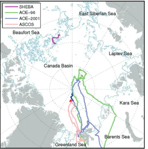
International Polar Year (IPY), with substantial international contributions. ASCOS was the most extensive in-situ atmospheric Arctic Ocean experiment during the IPY, lasting over a month in the North Atlantic sector of the Central Arctic Ocean. It was centered on a three-week ice-drift operation at∼87◦N from mid-August through the beginning of

September, with the icebreaker moored to a drifting ice floe. Figure 1 shows the track

20

of the expedition.

Process studies such as those conducted during ASCOS must be put into a larger context. The atmosphere is highly variable on many time scales and this gives rise to two main considerations. First, any findings from process-level observations must be interpreted within the context of the larger-scale atmospheric circulation. Second,

25

(7)

research-ACPD

12, 4101–4164, 2012

Title Page

Tables Figures

◭ ◮

Back Close

Full Screen / Esc

Discussion

P

a

per

|

Dis

cussion

P

a

per

|

Discussion

P

a

per

|

Discussio

n

P

a

per

|

quality cloud and surface flux observations. But because this is the only such data set, there is a risk they are assumed to represent a much larger area and time-frame. With an expedition as short as ASCOS this risk is obviously even greater. Therefore, new observations must be cautiously placed within the context of existing observations, e.g. satellite-based estimates or in-situ data from prior field experiments.

5

In this paper we present a summary of the meteorological conditions that were en-countered during ASCOS, from the synoptic scale down to boundary-layer scales, to aid in interpretation of process studies presented in many other papers. In doing this, we compare the ASCOS conditions with both climatological means and with obser-vations from three earlier summer experiments: the AOE-96, SHEBA and AOE-2001

10

expeditions. A brief description of ASCOS and the data used in this study is given in Sect. 2. In Sect. 3 we discuss the large-scale atmospheric setting and transport characteristics during ASCOS, while Sect. 4 presents some basic meteorological char-acteristics from ASCOS, comparing these to results from the other experiments. Sec-tion 5 describes some of the main characteristics of the ASCOS ice drift and Sect. 6

15

contains a brief summary and conclusions.

2 Data

2.1 The ASCOS experiment

The primary objective of ASCOS is to understand the formation and life cycle of low-level clouds and the role these play in the surface energy budget of the high Arctic,

20

especially during the transition from late summer to early fall. ASCOS was designed as an interdisciplinary project with science teams specializing in meteorology, physical oceanography, atmospheric gas-phase chemistry, particulate chemistry and physics, marine biology and biochemistry. Like its predecessors (I91, 96 and AOE-2001), ASCOS was conducted onboard the Swedish icebreakerOden. The expedition

(8)

ACPD

12, 4101–4164, 2012

Title Page

Tables Figures

◭ ◮

Back Close

Full Screen / Esc

Discussion

P

a

per

|

Dis

cussion

P

a

per

|

Discussion

P

a

per

|

Discussio

n

P

a

per

|

departed Longyearbyen on Svalbard on 2 August (DoY1214), returning on 9 Septem-ber (DoY 253), 2008. By 12 August (DoY 225), after a few brief research stations in open water and the marginal ice zone and a transit north into the pack ice,Odenwas moored to a 3_×6 km ice floe with which it drifted for 21 days. The drift track, from ap-proximately 87◦21′N, 01◦29′W to 87◦09′N, 11◦01′W, is illustrated in Fig. 1. A detailed

5

summary of the scientific background and details on all observations is contained in Tjernstr ¨om et al. (2011) and only a brief summary will be provided here.

Operational large-scale meteorological analysis and forecasts for the expedition were supplied by the European Centre for Medium Range Weather Forecasts (ECMWF) and the UK Met Offi_{ce; in this paper we use the ECMWF analyses while} 10

the UK Met Offi_{ce Unified Model forecasts are presented and analyzed in Birch et al.}

(2011). To compare ASCOS conditions to climatology we use the NCAR/NCEP reanalysis products, readily available from the National Oceanographic and Atmo-spheric Administration/Earth System Research Laboratory (NOAA/ESRL) web-site at http://www.esrl.noaa.gov/psd. Back-trajectories based on analyzed meteorological

15

fields calculated after the expedition, were obtained from HYSPLIT (http://ready.arl. noaa.gov/HYSPLIT.php).

Table 1 summarizes the diff_{erent sources of data from all four expeditions used in}

this study. For ASCOS, basic meteorology parameters were extracted from Oden’s

weather station, complemented by a WeatherPak installed onboard providing some

20

redundancy, and from the micro-meteorology deployment on the ice during the ice drift. Analyses of tropospheric vertical structure, clouds and frontal zones rest on the 6-hourly radiosoundings and on the MilliMeter wave-length Cloud Radar (MMCR) in-stalled on theOden. Additional information on the clouds comes from several laser ceilometers, and additional temperature profile information comes from a scanning

mi-25

crowave radiometer. Visibility is provided by a backscatter visibility sensor that was part of theOden weather station. Observations of surface radiation fluxes come from

1

(9)

ACPD

12, 4101–4164, 2012

Title Page

Tables Figures

◭ ◮

Back Close

Full Screen / Esc

Discussion

P

a

per

|

Dis

cussion

P

a

per

|

Discussion

P

a

per

|

Discussio

n

P

a

per

|

broadband pyranometers and pyrgeometers deployed on the ice, complemented by similar instruments on theOden; net surface radiation could only be measured on the ice. Turbulent heat fluxes were derived from eddy-correlation measurements made on two micrometeorology masts on the ice. Several other instrument systems were also deployed during ASCOS (see Tjernstr ¨om et al., 2011, for a complete description) but

5

are not used here.

2.2 Previous expeditions

Data from other expeditions are used to put ASCOS results into a broader context. This data comes from the AOE-96, SHEBA and AOE-2001 experiments (see Leck et al., 2001; Uttal et al., 2002; Tjernstr ¨om et al., 2004a,b, respectively, for

descrip-10

tions). ASCOS and the previousOden-based expeditions were of limited length and for diff_{erent, but overlapping, periods, while SHEBA was deployed for a full year. The}

overlapping time period for all expeditions is only 4–23 August, about three weeks. Di-rectly comparing observations from four diff_{erent years for such a brief period of time}

is diffi_{cult and perhaps not even meaningful. For this reason we instead consider the} 15

statistics of the diff_{erent observations, rather than comparing individual time series.}

With a primary interest in conditions during late summer and the early transition to autumn, we use all available observations within the perennial pack ice from the months of July and August from each experiment; this paper focuses on ASCOS so we extend the period 1 full day into September to include the end of the ASCOS ice

20

drift. In summary, we use all available observations made within the perennial pack ice between 00:00 UTC on 1 July and 00:00 UTC on 2 September. A consequence of using diff_{erent time periods is that some of the observations are biased towards}

the mid-summer melt period (e.g., SHEBA), while other may be dominated by the fall transition (e.g., ASCOS and AOE-96). Figure 2, showing the near-surface temperature

25

(10)

ACPD

12, 4101–4164, 2012

Title Page

Tables Figures

◭ ◮

Back Close

Full Screen / Esc

Discussion

P

a

per

|

Dis

cussion

P

a

per

|

Discussion

P

a

per

|

Discussio

n

P

a

per

|

south (Fig. 1).

As far as possible we have used the same, or similar, types of observations to com-pare diff_{erent parameters; see Table 1. However, for some parameters data is not}

available from all expeditions. In these cases the missing expedition is simply omitted. In other cases, diff_{erent types of observations or sensors were used for the same} ba-5

sic purpose. For example, cloud observations in SHEBA and ASCOS were obtained from the MMCR cloud radar, AOE-2001 deployed an S-band cloud and precipitation radar, while AOE-96 had no cloud radar. Also, while ASCOS, SHEBA and AOE-2001 had substantial ice drifts, AOE-96 had a very short ice-drift and data from the latter is omitted. The number of soundings included in the comparison diff_{ers, and there has} 10

been a significant development in radiosonde sensor technology between 1996 and 2008. Thus, diff_{erences in time, frequency and quality of the observations, must be}

born in mind during the following analysis. It is not the intention of this paper to estab-lish a “summer Central Arctic climatology”. However, we do believe that some similar characteristic have been observed.

15

3 Large-scale atmospheric setting during ASCOS

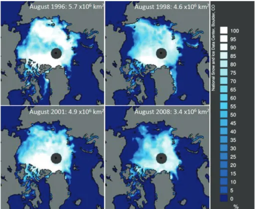
Figure 3 shows the mean sea-ice area cover from the National Snow and Ice Data Center (NSIDC) for August of each experimental year. The general trend is of decreas-ing summer sea ice extent with time: 1996 had the largest total area cover and 2008 the smallest. There are also interannual diff_{erences in the regional location of the pack} 20

ice. For example, the ice edge was far north in the Alaskan/East-Siberian sector during 1998 (the SHEBA summer) and again in 2008, while being farther south in 1996 and 2001. The ice fraction around the pole is lowest in 1996, consistent with reports of many open leads (Leck et al., 2001), and low again in 2008.

The synoptic-scale atmospheric circulation exhibits large interannual variability, thus

25

(11)

ACPD

12, 4101–4164, 2012

Title Page

Tables Figures

◭ ◮

Back Close

Full Screen / Esc

Discussion

P

a

per

|

Dis

cussion

P

a

per

|

Discussion

P

a

per

|

Discussio

n

P

a

per

|

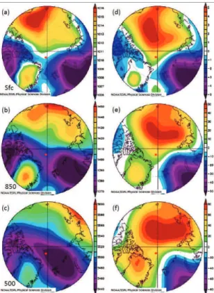
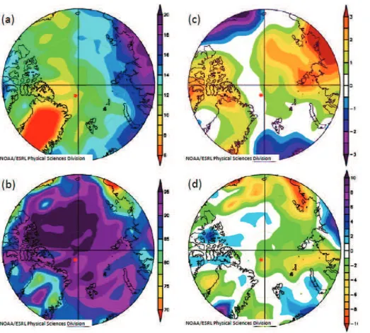
features of the large-scale atmospheric circulation during ASCOS, as manifested by the mean-sea-level pressure (MSLP) and the 850 and 500 hPa geopotential height fields (Fig. 4a–c) and their anomaly compared to the 1981–2010 climatology over the same time period (Fig. 4d–f). The MSLP (Fig. 4a) features a high-pressure region over the North-American and Siberian quadrants with a center over the Canada Basin

5

and a separate high-pressure center over Greenland. Low pressure centers are lo-cated over the Barents and Nordic Seas and over the Canadian Archipelago. While the Greenland high-pressure center is consistent with the climatology, the pressure pattern over the Arctic Ocean is anomalous (Fig. 4d), with a positive anomaly of up to 5–6 hPa over the Canada Basin and a similar negative anomaly over the Barents

10

Sea. This implies an easterly surface-flow anomaly over much of the ASCOS region, which is consistent with the more detailed synoptic-scale analysis below. The low-pressure region remains at approximately the same horizontal location in the vertical while broadening somewhat across Northern Greenland and the high-pressure region moves gradually westward in over Siberia with altitude. The anomaly is thus nearly

15

barotropic in character and exhibits about the same spatial structure on both pressure surfaces (Fig. 4e,f), while the pressure field itself is baroclinic.

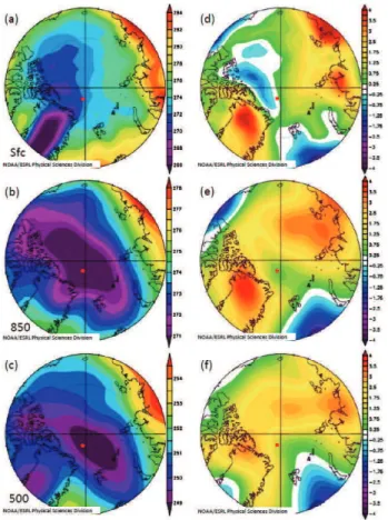
Figure 5 shows the temperature fields and its anomalies. The region with the low-est temperature tilt with height across the Arctic from the Beaufort Sea at the surface, centered on the North Pole at 850 hPa and located north of Svalbard at 500 hPa. The

20

temperature anomaly displays a dipole pattern with high near-surface temperatures over Greenland and Siberia, marginally low temperatures on the Canadian side of the Arctic Ocean, but a bridge of positive temperature anomaly from Greenland to Siberia strengthening with altitude. Precipitable water (Fig. 6) is high over Siberia and low over Greenland; the high values over Siberia are an anomaly while conditions over

Green-25

(12)

ACPD

12, 4101–4164, 2012

Title Page

Tables Figures

◭ ◮

Back Close

Full Screen / Esc

Discussion

P

a

per

|

Dis

cussion

P

a

per

|

Discussion

P

a

per

|

Discussio

n

P

a

per

|

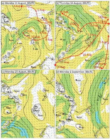
Figure 7 illustrates details of the synoptic scale weather during ASCOS. A select set of ECMWF surface pressure and wind analyses are shown, complemented by 12-hourly storm tracks for the most significant weather systems. During the first part of the expedition several significant storms moving from east to west passed the ASCOS track, the opposite of the usual direction of travel and consistent with the MSLP

anoma-5

lies (Fig. 4d). Figure 7a shows the first, starting on 4 August (DoY 217) in the Canada basin, moving to the Kara Sea by 7 and 8 August (DoY 220 and 221), crossing over Svalbard on 10 August and then passing ASCOS on 12 August (DoY 225). This was the first day of the ice drift and this weather system slowed down the initial deploy-ment of instrudeploy-mentation on the ice, bringing strong winds, precipitation and generally

10

adverse conditions for working on the ice.

The next weather system (Fig. 7b) started on 12 August (DoY 225) over the Kara Sea and then moved rapidly westwards passing south of the ASCOS ice drift on 14 and 15 August (DoY 227 and 228) and dissipated north of the Canadian Archipelago. The flow then changed character, with two storms passing rapidly eastward across the

15

Nordic, Greenland and Kara Seas without aff_{ecting ASCOS. After this, the}

synoptic-scale weather became more quiescent, with the formation of a high-pressure system over Svalbard (Fig. 7c,d), which moved slowly towards and across the North Pole. A secondary high pressure over Greenland created a common omega-shaped block-ing pattern over the North Atlantic. Towards the end of the ice drift an extensive and

20

intense low-pressure system developed over the Kara Sea and moved westward to-wards Svalbard (Fig. 7d). This did not aff_{ect the ASCOS observations until after the ice}

drift had been terminated and theOdenwas moving south in the open Greenland Sea towards Longyearbyen.

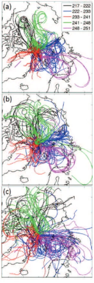
Figure 8 shows back-trajectories with receptor points at the location ofOdenat 100,

25

(13)

ACPD

12, 4101–4164, 2012

Title Page

Tables Figures

◭ ◮

Back Close

Full Screen / Esc

Discussion

P

a

per

|

Dis

cussion

P

a

per

|

Discussion

P

a

per

|

Discussio

n

P

a

per

|

be identified. Early in the expedition, whileOdenwas moving north towards and into the ice (4–9 August; DoY 217–222) the air approaching ASCOS predominantly arrived from the ice covered region north of Canada and Alaska. Conditions then changed and during 9–20 August (DoY 222–233) the origin of the air was highly variable on a daily time scale but mostly came from the Greenland, Barents and Kara Seas; this

5

was the synoptically very active period discussed above (see Fig. 7a,b). A new shift oc-curred around 20 August (DoY 233), with a period when trajectories reaching ASCOS mostly originated in the vicinity of Greenland. Through the end of the ice drift and the beginning of the traverse back to the Greenland Sea (28 August–4 September; DoY 241–248) the origin of the air swings around to come from across the Central Arctic.

10

At the end of the campaign (DoY 248–251), the origin of the air was again from the Kara Sea and adjacent land. Many of these shifts are clearly distinguishable in the observations.

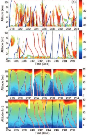
Figure 9 shows a subjective analysis of passing frontal disturbances associated with the synoptic-scale weather systems, overlaid onto both the MMCR cloud radar

re-15

flectivity (Fig. 9a) and the equivalent potential temperature2,Θ

e, from the soundings

(Fig. 9b). The dashed vertical lines indicate the beginning and end of the ice-drift pe-riod. The subjective analysis is produced using the time-rate-of-change and the slope with height ofΘ

e, aided by the MMCR cloud reflectivity. The most intensive period of

weather systems is roughly from 6 through 21 August (DoY 219–234). The most

sig-20

nificant set of fronts is associated with the synoptic scale disturbance that arrived on 12 August (DoY 225). This period ended with a weather system on 20 August (DoY 233), followed by a two day period with only low-level cloud or fog which ended on 23 August (DoY 236) with another weather system; depending on definition either of these

2_Θ

e= Θ + L

Θ

CpTq, where

Θ_{is the potential temperature defined as}Θ =_T₍_p/₁₀₀₀₎ Rd

cp_,_T _{is the}

temperature,p is the pressure, Rd andcp are the gas constant and heat capacity of dry air,

respectively,Lis the latent heat of vaporization andqis the specific humidity. Note that the tem-perature (T) in the definition ofΘ

eis evaluated at the lifting condensation level in unsaturated

(14)

ACPD

12, 4101–4164, 2012

Title Page

Tables Figures

◭ ◮

Back Close

Full Screen / Esc

Discussion

P

a

per

|

Dis

cussion

P

a

per

|

Discussion

P

a

per

|

Discussio

n

P

a

per

|

weather systems marked the end of the melt season (Sedlar et al., 2011a; Sirevaag et al., 2011; , Persson et al 2012); see Sect. 5. Thereafter follows a more quies-cent period from 23 August through 3 September (DoY 236–247) under the influence of a high-pressure system with several embedded weak frontal passages; favorable conditions for a persistent stratocumulus layer residing in the subsidence inversion.

5

Following this, synoptically more active weather reappears as ASCOS nears its end. The diff_{erent periods observed during the ice drift will be discussed in detail in Sect. 5.}

4 Meteorological conditions encountered during ASCOS

4.1 Basic meteorological variables

In this section we present key meteorological variables from ASCOS. A comparison to

10

observations from earlier expeditions is included to put ASCOS results in context. Fig-ure 2 shows time series of near-surface temperatFig-ure from the four expeditions. Near-surface temperature during July (DoY 183–213) remains close to 0◦_{C, as expected for}

the melt season, when all excess heating contributes to melting of ice and snow rather than to a surface warming. Through August (DoY 212–243) all four time series show

15

a gradual decrease in temperature with time, along with the occurrence of brief colder periods lasting for up to several days. These periods appear to be a common feature, perhaps signaling the oncoming transition to fall freeze-up conditions, and have been associated with periodic breaks or reductions in cloud cover (Tjernstr ¨om, 2005; Sedlar et al., 2011a).

20

Figure 10 shows the relative probability of near-surface temperature, relative humid-ity and wind speed. In generating these statistics from the threeOden-based expe-ditions, we used both the ship’s weather station and observations made on the ice during the ice-drifts (absent for AOE-96). For SHEBA we used only observations from the mast on the ice (e.g., Persson et al., 2002). TheOdenweather station was located

25

(15)

ACPD

12, 4101–4164, 2012

Title Page

Tables Figures

◭ ◮

Back Close

Full Screen / Esc

Discussion

P

a

per

|

Dis

cussion

P

a

per

|

Discussion

P

a

per

|

Discussio

n

P

a

per

|

between the expeditions, generally in the 5–15 m interval.

Temperatures during ASCOS were mostly in the−2 to 0◦C range, which is roughly

the interval between the freezing points of saline (ocean) water and fresh (snow on top of the ice) water and is typical for the melt season. The ice-drift measurements also clearly reflect the two periods of lower temperatures around DoY 235 and 245.

5

The statistics from the other four expeditions are very similar. The temperatures from SHEBA are the warmest and peak at a slightly positive temperature, while those from AOE-96 are the coolest, with a broad peak around ∼ −1.5◦C. All distributions have

a negative tail, SHEBA the least and ASCOS and AOE-96 the most. These are a reflec-tion of the temporary drops in temperature that predominantly appeared in August. The

10

fact that SHEBA is somewhat warmer is a consequence of including the whole month of July, which is somewhat warmer on average; SHEBA is also at a more southerly lo-cation. Leck et al. (2001) report that AOE-96 was an unusually cloud free and attribute the cooler temperatures to the lack of positive cloud radiative forcing. The ASCOS near-surface conditions were also very moist (Fig. 10b), with the most commonly

oc-15

curring near-surface relative humidity close to 100 %, and almost no cases where it dropped below 90 %. ASCOS conditions fall in the middle of these expeditions with SHEBA, followed by AOE-2001, being the most humid. AOE-96 is again slightly diff

er-ent, with somewhat lower relative humidity peaking at 96 %, consistent with the lower clouds amounts and thus cooler temperatures.

20

The wind speed does not have any constraints similar to that for temperature and moisture, and is consequently more variable. For ASCOS the winds were significantly weaker when considering only the ice drift than for the whole expedition (Fig. 10c). This is a manifestation of the generally more synoptically active period at the beginning of the expedition, ending a few days into the ice drift. The most common wind speeds

25

for the whole expedition were 3–5 m s−1, with a weak secondary peak at 10 m s−1and no cases of winds>16 m s−1_{. The ice drift was significantly calmer with winds mostly}

(16)

ACPD

12, 4101–4164, 2012

Title Page

Tables Figures

◭ ◮

Back Close

Full Screen / Esc

Discussion

P

a

per

|

Dis

cussion

P

a

per

|

Discussion

P

a

per

|

Discussio

n

P

a

per

|

made on the ship. A comparison of ship-borne and mast-borne measurements from ASCOS, only using data from periods when they coexist, suggests that the height of the measurement makes only a small diff_{erence (not shown). Comparing the}

expedi-tions, the SHEBA record has the lowest winds, while AOE-2001 has the highest, with ASCOS in between. The peak in the AOE-96 statistics is similar to that from SHEBA,

5

but there is also a secondary peak at higher wind speeds. In general, across all the ex-peditions, wind speeds were commonly 2–8 m s−1, seldom above 10 m s−1and hardly ever exceeding 15 m s−1_.

4.2 Vertical structure

The vertical thermodynamic structure of the lower atmosphere (<4 km) was

evalu-10

ated from the radiosoundings. Figure 11 shows the probability of equivalent potential temperature,Θ

e, as a function of altitude. A constant value with height signifies

near-neutral moist-static stability conditions, while increasing values are statically stable. Figure 12 shows similar statistics for relative humidity (RH). A dominating feature from ASCOS was a pronounced near-neutrally stratified layer in the lowest atmosphere,

15

from the surface up to _∼500 m (Fig. 11a), accompanied with high relative humidity, generally RH>95 %, in a layer from the surface up to about 1 km (Fig. 12a). This is consistent with the observation that specific humidity increases across the boundary-layer inversion (Tjernstr ¨om et al., 2004a; Tjernstr ¨om, 2005; Devasthale et al., 2011). With increasing temperature with height, if the relative humidity is constantly high, it

20

follows that as temperature increases into the inversion specific moisture must also increase. It also suggests the possibility that clouds may penetrate into the lower in-version, rather than being capped by it. This structure has been found to be common in cloud radar and temperature profiles from AOE-2001, ASCOS, SHEBA and Bar-row, Alaska (Sedlar and Tjernstr ¨om, 2009; Sedlar et al., 2011b), and recognized as

25

(17)

ACPD

12, 4101–4164, 2012

Title Page

Tables Figures

◭ ◮

Back Close

Full Screen / Esc

Discussion

P

a

per

|

Dis

cussion

P

a

per

|

Discussion

P

a

per

|

Discussio

n

P

a

per

|

atmosphere ranged from 300–400 m in AOE-2001 and AOE-96 to ∼400 m during

SHEBA (Fig. 11b–d); ASCOS thus featured the deepest neutrally stratified layer. Dur-ing ASCOS (Fig. 11a) well-mixed surface layers appeared preferentially at two temper-atures, around Θ

e∼9◦C and at a lower temperature of Θe∼3◦C. A similar feature,

although weaker, was present also in AOE-96 (Fig. 11c). In both cases the colder

5

structures were shallower. During AOE-96 and SHEBA, the boundary-layer tempera-ture was slightly lower, atΘ

e∼7–8◦C. All the expeditions also had very high relative

humidity in the lowest troposphere, >95 % (Fig. 12b–d). The highest relative humid-ity was observed during SHEBA, being even higher than during ASCOS (Fig. 12a,d), while the lowest values were found in AOE-2001 (Fig. 12b). The moist layer is also

10

deeper than the well-mixed layer for all expeditions often reaching to>1 km. SHEBA had the deepest moist layer, slightly deeper than ASCOS, while AOE-96 had the most shallow layer,∼500 m. The lower troposphere stratification is thus very similar in all

four expeditions.

The characteristics of the capping inversion are illustrated in Fig. 13, showing the

15

base height of the capping inversion, and its thickness, strength and static stability. This analysis is based on scanning radiometer temperature profiles from ASCOS and AOE-2001, and on radiosoundings for SHEBA. The objective algorithm applied to the temperature profiles to determine the inversions is that of Tjernstr ¨om and Graversen (2009); the main inversion is defined as that with the strongest stability and there is

20

a very clear correlation between strength, stability and depth (not shown). Note that with this data, inversions with a base below but a top above 1.2 km (the maximum height of the scanning radiometer) will be represented in the inversion base statistics, but not in the statistics for thickness and strength. Over 95 % of all analyzed pro-files feature at least one main inversion (e.g., Tjernstr ¨om 2005, 2007; Tjernstr ¨om and

25

Graversen, 2009) and multiple inversions in the lowest kilometer were common. The absolute peak in the probability for the height to base of the main inversion (Fig. 13a) in ASCOS occurred at∼100 m, however, for the rest of the altitude interval the

(18)

ACPD

12, 4101–4164, 2012

Title Page

Tables Figures

◭ ◮

Back Close

Full Screen / Esc

Discussion

P

a

per

|

Dis

cussion

P

a

per

|

Discussion

P

a

per

|

Discussio

n

P

a

per

|

about at about the same frequency. The thickness of ASCOS inversion were most often around 100–300 m, and the probability function for inversion strength was broad,

∆_T_∼_1–6◦_C.

Comparing to other expeditions, both SHEBA and AOE-2001 had more distinct low-level peaks for the inversion base heights with AOE-2001 somewhat higher, at_∼200 m,

5

and SHEBA slightly lower. In neither of these were there any significant occurrences of inversion bases above∼800 m. Both SHEBA and AOE-2001 had more occurrences

of thicker inversions, with a broader peak from 100 to 600 m (Fig. 13b), and while AOE-2001 had significantly more weak inversions with pronounced peak at∆_T _∼₁◦_C

(Fig. 13c), SHEBA had similar inversion strengths compared to ASCOS. Inversions

10

never exceed∆_T_∼₁₂◦_{C in any of the expeditions. In terms of stability, combining the}

strength and depth for the individual inversions (Fig. 13d), ASCOS and SHEBA were very similar, while AOE-2001 inversions had significantly weaker stability.

Figure 14 shows median profiles of temperature, specific humidity and wind speed for all four expeditions. The median temperature profiles (Fig. 14a) exhibited a well-mixed

15

near-surface layer, the deepest during ASCOS and shallowest in AOE-2001, capped by an inversion – strongest and deepest in AOE-2001 and weakest and highest during ASCOS while AOE-96 and SHEBA are very similar. AOE-96 also had a slightly higher stability near the surface. The specific humidity (Fig. 14b) varied considerably between the expeditions and is the lowest in AOE-96, consistent with the subjective impressions

20

of less clouds and cooler conditions in AOE-96. SHEBA was moistest, with a significant layer of higher values between∼400 m and∼1.2 km.

Wind speeds in the lower troposphere, below 1–2 km, were highest during AOE-96 (_∼8 m s−1) and the lowest in AOE-2001 (_∼5 m s−1) with ASCOS and SHEBA being similar at ∼6 m s−1 (Fig. 14c). AOE-96, and possibly ASCOS, had weak low-level 25

(19)

ACPD

12, 4101–4164, 2012

Title Page

Tables Figures

◭ ◮

Back Close

Full Screen / Esc

Discussion

P

a

per

|

Dis

cussion

P

a

per

|

Discussion

P

a

per

|

Discussio

n

P

a

per

|

Oden-based expeditions encountered significantly higher median wind speeds than did SHEBA, at 15–20 m s−1_and

∼10 m s−1, respectively, with ASCOS having the highest

values. Although the sample is very small, such a diff_{erence may be a consequence}

of the diff_{erences in location. In this upper-troposphere layer ASCOS also had the}

highest and AOE-96 the second lowest wind speeds, with AOE-2001 in between.

As-5

suming that the wind-speed increase with height across the troposphere is a proxy for baroclinic instability, these diff_{erences might reflect di}ff_{erences in synoptic-scale}

ac-tivity between the two regions, the Beaufort Sea for the SHEBA deployment and the Atlantic sector of the Central Arctic where theOden-based expeditions were deployed, and diff_{erences between the di}ff_{erent years in the latter.}

10

4.3 Clouds

For the purpose of this study, “a cloud” is defined by the instruments used for de-tecting it (see discussion in Shupe et al., 2011). For ASCOS and AOE-2001 cloud fractional occurrence was estimated using ceilometer data, while during SHEBA cloud-occurrence statistics was estimated using a multi-sensor approach, including lidar and

15

cloud radar. With this in mind, ASCOS and AOE-2001 cloud occurrence fractions might be underestimated since they use only a single sensor with lower sensitivity at higher altitudes. Note also that cloud fraction is defined using zenith-viewing instruments, sensing clouds as a function of time as they pass above, and thus not estimating the actual spatial cloud cover at any given time.

20

Several studies have indicated large amounts of low-level cloud in the Arctic during summer (e.g., Wang and Key, 2005; Karlsson and Svensson, 2010). For ASCOS the average total cloud fraction was about 90 % while the boundary layer cloud fraction was about 80 %. During AOE-2001 the average total cloud cover was 85 %, and 80 % for boundary-layer clouds. Shupe et al. (2011) reports a mean cloud fraction from 90

25

(20)

ACPD

12, 4101–4164, 2012

Title Page

Tables Figures

◭ ◮

Back Close

Full Screen / Esc

Discussion

P

a

per

|

Dis

cussion

P

a

per

|

Discussion

P

a

per

|

Discussio

n

P

a

per

|

Figure 15 shows statistics of cloud geometry. Here the cloud base is defined by the lowest indication of a cloud from the ceilometer or the cloud radar, whichever is the highest, while the cloud top is obtained from cloud radar. For SHEBA, only occur-rences with single-layer clouds are used. These totally dominated in August; in July single-layer clouds were the most common, while there were more cases with multiple

5

cloud layers (Intrieri et al., 2002). The height of the lowest cloud base (Fig. 15a) has a pronounced low-level maximum in all four experiments, peaking at<100 m, while the lowest cloud tops (Fig. 15b) usually occur below 1 km, with a maximum between 200 and 800 m for the threeOdenexpeditions. SHEBA also has a secondary peak of low-est cloud-top around∼1 km. Figure 15c shows statistics of estimated cloud thickness: 10

for ASCOS and AOE-2001 this has a maximum around 300 m, with very few clouds thicker than 1 km. SHEBA has a more uniform distribution between 300 m and_∼1 km. ASCOS and SHEBA carried passive dual-wavelength microwave radiometers that continuously monitor vertically-integrated column water vapor (precipitable water) and liquid water path, the vertically integrated cloud water content (Westwater et al., 2001).

15

Both expeditions also deployed the MMCR cloud radar, facilitating an estimate of in-tegrated cloud ice (Shupe et al., 2005). Figure 16 shows these three measures for ASCOS and SHEBA. The total column water vapor distributions (Fig. 16a) are very similar, with the SHEBA results shifted to somewhat moister conditions, possibly a con-sequence of SHEBA’s more southerly location. In terms of cloud water (Fig. 16b,c),

20

ASCOS has significantly more cloud liquid than SHEBA but less cloud ice.

Figure 17 shows the probability distribution of the visibility from the backscatter vis-ibility sensor; for SHEBA this information is not available. All three exhibit similar be-havior, with peaks below 1 km (the threshold for fog conditions according to the WMO definition) and for visibility>20–30 km. Note that visibility can also be low in snowfall,

25

(21)

ACPD

12, 4101–4164, 2012

Title Page

Tables Figures

◭ ◮

Back Close

Full Screen / Esc

Discussion

P

a

per

|

Dis

cussion

P

a

per

|

Discussion

P

a

per

|

Discussio

n

P

a

per

|

<100 %, was essentially non-existent.

4.4 Surface energy fluxes

Incoming (downward) long- and shortwave radiation is strongly aff_{ected by clouds and}

was observed onboard the ship during the threeOden expeditions, on the ice during the AOE-2001 and ASCOS ice-drifts, and continuously on the ice during SHEBA. The

5

upward radiative fluxes (and thus net fluxes) are only available from observations on the ice.

During ASCOS the incoming solar radiation (Fig. 18a) peaked at approximately 50– 100 W m−2_{from both the longer ship record and the observations from the ice, with very}

few values>200 W m−2_{. For net solar radiation at the surface (Fig. 18b) the distribution}

10

from ASCOS had a sharp peak at∼10 W m−2, with few values>50 W m−2. Incoming

longwave radiation (Fig. 18c) had a peak around 300–310 W m−2_{with a sharper}

some-what lower peak when considering only the ice drift. There was a long tail towards lower values, down to 200–220 W m−2. The net longwave radiation had a sharp peak at−10 W m−2 with a negative tail down to∼ −60 W m−2. This behavior with quite dis-15

tinct peaks and long tails is a result of the impact of the clouds on the radiation; the peaks represent the usually cloudy conditions while the tails, negative for net longwave and positive for net shortwave, reflects the relatively few and short clear periods.

Comparing to the other expeditions, there are similarities and some diff_erences.

In-coming solar radiation for the longer ship record at AOE-2001 peaked at 140 W m−2,

20

while its ice drift probability peaked at slightly lower values, at∼100 W m−2, and the

distribution was narrower. AOE-96 had peak values similar to ASCOS, but with a wider distribution, while SHEBA conditions had a much wider distribution with a flat peak around 10–80 W m−2 and a long positive tail. For net solar radiation at the surface (Fig. 18b) the distributions from ASCOS and AOE-2001 were similar but with higher

25

peak values for AOE-2001 by about 10 W m−2; both had similar tails with few values

>50 W m−2. SHEBA was again diff_{erent, peaking at}_∼_{10 W m}−2_{and exhibiting a broad}

(22)

ACPD

12, 4101–4164, 2012

Title Page

Tables Figures

◭ ◮

Back Close

Full Screen / Esc

Discussion

P

a

per

|

Dis

cussion

P

a

per

|

Discussion

P

a

per

|

Discussio

n

P

a

per

|

located farther south and had a smaller LWP than ASCOS (Fig. 16b), both of which contribute to higher incoming solar radiation. In addition to a lower LWP, SHEBA had significantly more melt ponds during summer than at both AOE-2001 and ASCOS, likely causing a lower surface albedo. The incoming longwave radiation (Fig. 18c) was more similar across the four expeditions, with peaks in the 300–320 W m−2_range,

5

SHEBA being marginally higher, while the larger occurrence of lower values in AOE-96 reflects more clear conditions. The same is true also for net longwave (Fig. 18d), with peaks around ₋10 to 0 W m−2_{. SHEBA had a somewhat broader distribution and an}

absolute peak at a few W m−2 (positive), and more frequent occurrences of values in the−10–−20 W m−2range.

10

Turbulent surface heat fluxes in the Arctic are generally small (e.g., Persson et al., 2002; Tjernstr ¨om, 2005). In Fig. 19a,b statistics of the turbulent surface energy fluxes for ASCOS are compared to AOE-2001 and SHEBA; upward fluxes are defined posi-tive. The sensible heat flux (Fig. 19a) during the ASCOS ice drift had a sharp peak in probability around zero, with both positive and negative tails. The positive tail was the

15

more substantial, up to 10 W m−2, while the negative tail, down to−5 W m−2, was less

pronounced. The distributions for the AOE-2001 and SHEBA sensible heat fluxes were quite similar, peaking around zero, and the tails were more pronounced and evenly dis-tributed,±7–8 W m−2, compared to ASCOS.

The latent heat flux time series are shorter because of diffi_{culties in measuring the} 20

flux in the Arctic among other things owing to accumulation of ice frost and riming on the optical surfaces of the open path sensors used in all these experiments. As this would occur mostly in cases with a downward directed flux of water vapor, exclusion of such episodes may have biased the result. ASCOS and SHEBA fluxes were mostly positive (Fig. 19b) indicating that evaporation is most common, although maximum

25

values are small,∼5 W m−2. AOE-2001 has more cases with a downward latent heat

(23)

ACPD

12, 4101–4164, 2012

Title Page

Tables Figures

◭ ◮

Back Close

Full Screen / Esc

Discussion

P

a

per

|

Dis

cussion

P

a

per

|

Discussion

P

a

per

|

Discussio

n

P

a

per

|

height intervals, depending on the deployment of the instruments (within 8–15 m above the surface). These are relatively similar for all expeditions, with near-neutral conditions being the most common. ASCOS was more frequently unstably stratified than AOE-2001 or SHEBA, consistent with the sensible heat flux (Fig. 19a).

5 Characteristics of the ASCOS ice drift

5

The ice drift of ASCOS took place roughly between 00:00 UTC 13 August (DoY 225) and 00:00 UTC 2 September (DoY 246), although diff_{erent instrument systems came}

on line gradually over the first few days, and the tear-down progressively reduced in-strumentation during the last day. The eff_{ective length of the ice drift is illustrated in}

Fig. 20a showing time series of several temperatures near the surface (air temperature

10

at 3.2 m and a set of surface temperatures). Sedlar et al. (2011a) analyzed the surface energy budget and defined four main periods for the ice drift with diff_erent

character-istics; here we refine these definitions and additionally divide their first period into two for a total of five periods, which are discussed below and in Figs. 20–24.

Figure 20a shows that the first two periods were somewhat typical for the melt

sea-15

son. Both had a significant excess of surface energy, as analyzed by Sedlar et al. (2011a), that could melt ice and snow at the surface, however, the 1st period was sig-nificantly more variable in temperature than the second. Figure 20b shows the cloud radar reflectivity and reveals a more synoptically active 1st period compared to the 2nd, although both were aff_{ected by several weather systems as manifested by the} 20

deep frontal cloud structures, especially 12–13 and _∼16 August (DoY 225–226 and 229), with three more minor systems in between. Both periods have a high cloud frac-tion within the lowest kilometer and also a significant amount of higher cloud, the 1st period more so than the 2nd.

A weather system at the end of the 2nd period (20 August; DoY 233) marks the

25

(24)

ACPD

12, 4101–4164, 2012

Title Page

Tables Figures

◭ ◮

Back Close

Full Screen / Esc

Discussion

P

a

per

|

Dis

cussion

P

a

per

|

Discussion

P

a

per

|

Discussio

n

P

a

per

|

2.5 days (Fig. 20a). Relatively large cloud fractions were associated with this period, although clouds was mostly limited to below 400–500 m. The cloud fraction aloft mostly remained below 30 % with a slight increase around 6–8 km due to the optically thin cirrus cloud seen in Fig. 20b during this period. The surface albedo first increased due to fresh snow from the weather system on the 20th. During the 3rd period, freezing of

5

melt ponds and some of the open (saline) water surface, along with heavy riming and frost deposits, increased the surface albedo further (Sedlar et al., 2011a). A weather system on 23 August (DoY 236) additionally covered the surface with layer of new snow. The transmission of solar radiation through the ice also went through an abrupt change on 24 August (Sedlar et al., 2011a; Sirevaag et al., 2011); this also ended the

10

3rd period. The surface albedo increased from∼70 % to∼85 % from before to after

the 3rd period (not shown) and the surface energy balance did not recover to positive values again.

Surface temperature remained around the freezing point of ocean salt water during the whole 4th period (approximately₋2◦_{C, Fig. 20a). This period was characterized}

15

by relatively steady conditions, with a significant diurnal cycle in near-surface temper-ature that now became possible because the variations in surface tempertemper-ature are not limited by the melting point of fresh water. Conditions were governed by a quasi-steady high-pressure system (see Fig. 7d), and the dominating feature was a persis-tent stratocumulus layer. The 4th period thus had a high cloud fraction below 1 km,

20

and approximately 10% cloud cover on average in the free troposphere (Fig. 20b). The clouds contributed to the maintenance of the surface energy balance close to zero through surface cloud-radiative forcing (Sedlar et al., 2011a). As a consequence, the actual transition to the autumn freeze-up was postponed until the end of the 4th period (Fig. 20a). While the height to the top of these clouds was variable in time, towards

25

(25)

ACPD

12, 4101–4164, 2012

Title Page

Tables Figures

◭ ◮

Back Close

Full Screen / Esc

Discussion

P

a

per

|

Dis

cussion

P

a

per

|

Discussion

P

a

per

|

Discussio

n

P

a

per

|

temperature rapidly dropped to−12◦C, although there was a temporary recovery of the

temperature due to reappearing low-level clouds midday on 1st September (DoY 245) (see remaining surface temperature in Fig. 20a, after the mast had been taken down). The ice-drift was terminated at midnight between 1 and 2 September (DoY 246.0) but available observations suggest that the surface remained frozen after this (not shown).

5

Determining the onset of the freeze depends on the definition used. Many studies of diff_{erent types, using di}ff_{erent instrumentation, show a general consensus that the}

Central Arctic freeze onset often occurs between the 2nd week of August and early September (e.g., Rigor et al., 2000; Belchansky et al., 2004; Overland et al., 2008). One definition is the first time that a running-mean near-surface air temperature falls

10

below a somewhat arbitrary threshold, e.g.₋2◦_{C, to identify the freeze onset. In Fig. 20}

the near-surface air temperature, low-pass filtered at a cutoff_{frequency of two weeks,}

is shown as the dashed red line. It passes below this threshold at DoY 236 (23 August) consistent with the picture that freeze onset was triggered by the cold 3rd period and solidified by the change in albedo by the snowfall associated with the weather system

15

on DoY 236 (23 August). Note however that the exact timing of −2◦C crossing is

sensitive to the exact specifications in the low-pass filter design. The actual freeze started almost a week later, when the low-level clouds broke up, allowing the surface to cool rapidly in the longwave (Sedlar et al., 2011a). In essence this means that the end of the melt and the beginning of the freeze did not necessarily coincide. Regardless

20

of the definition used and exact date of end-of-melt/freeze-up, it is clear that ASCOS succeeded in capturing this important transition for 2008 during the ice drift.

The thermodynamic vertical structure of the five periods is illustrated by statistics of the profiles of equivalent potential temperature,Θ

e, and relative humidity with respect

to ice, RH_i, in Figs. 21 and 22; Figs. 23 and 24 show median profiles of wind speed,

25

and the vertical gradients ofΘ

eand scalar wind speed for the five periods, respectively.

The first two periods were similar in thermodynamical structure, while slightly diff_erent

(26)

ACPD

12, 4101–4164, 2012

Title Page

Tables Figures

◭ ◮

Back Close

Full Screen / Esc

Discussion

P

a

per

|

Dis

cussion

P

a

per

|

Discussion

P

a

per

|

Discussio

n

P

a

per

|

(to ∼100–200 m) and the moist layer deeper (to ∼1 km). The wind speeds during

the 1st period (Fig. 23) were significantly larger than during any of the other periods, including the 2nd. The temperature gradient from the first period (Fig. 24a) shows a shallow layer of unstable stratification close to the surface, approximately 70 m deep, with a near-neutral but slightly stable layer up to 300–500 m. The wind-speed gradient

5

during this period, although the largest during the ice drift, approaches zero at about

∼300 m (Fig. 24b). Thus even during in the 1st period, which had the most unstable

conditions close to the surface and the largest wind shear, the surface-based boundary-layer was limited to about 300 m. The well-mixed boundary-layer in the 1st period was topped by a stably stratified layer that extended from about 500 m, up to the capping inversion at

10

about 1 km (Fig. 24a). The 2nd period was slightly more stably stratified close to the surface, near-neutral up to 200 m. Then it becomes gradually more stable up to_∼1 km; above this the structure is similar to the 1st period.

The 3rd period, although signified by lower near-surface temperatures, was still well-mixed near the surface, but only in the lowest _∼50 m. This layer was capped

15

by a strong inversion extending to 400–500 m with free-tropospheric conditions aloft (Figs. 21c and 24a). The corresponding moist layer was∼200 m deep and the RHi

in this layer was >100 % (Fig. 22c) consistent with the formation of frozen drizzle in the low-level cloud layer and the accumulation of rime and frost on the surface. The wind speed was the lowest during the ice drift (Fig. 23) with an indication of a weak

20

low-level wind-speed maximum around 100–200 m. Consistent with this jet-like feature the wind-speed gradient crossed zero around 150 m and was negative but small up to

∼300 m (Fig. 24b).

The 4th period had a somewhat deeper and only slightly stable near-neutral layer in the lowest 100 m and then was more stable but still near-neutral in the 200–800 m

25

layer with a capping inversion at∼1 km. A clear double structure is visible in bothΘe

(27)

ACPD

12, 4101–4164, 2012

Title Page

Tables Figures

◭ ◮

Back Close

Full Screen / Esc

Discussion

P

a

per

|

Dis

cussion

P

a

per

|

Discussion

P

a

per

|

Discussio

n

P

a

per

|

upper of these well-mixed structures was associated with the stratocumulus cloud layer that was present for most of the 4th period. The wind shear during this period was zero above 200 m (Fig. 24b).

The 5th and final period displays a strong surface-based inversion up to ∼100 m,

by far the most stably stratified boundary layer during the ice drift, and is capped by

5

a secondary inversion starting at 300 m and transitioning to free tropospheric condi-tions above 800 m (Figs. 21e and 24b). The second stable layer 100–500 m was likely the remnants of the dissipating subsidence inversion in which the stratocumulus layer was previously residing. As the cloud dissipated, the buoyancy-generated turbulence from the cloud, forced by cloud-top cooling, has dissipated and the layer was becoming

10

increasingly stably stratified. The wind speed in the lowest kilometer increased during the 5th period and is the second strongest during the ice drift (Fig. 23) although the winds aloft are weaker and comparable to periods 2 and 4. The wind shear first ap-proaches zero at around 150 m with a 100 m shallow layer of negative shear on top (Fig. 24a).

15

The 4th period is of special interest with its persistent stratocumulus layer and the deep boundary layer with two distinct well-mixed layers in the thermodynamical struc-ture. Since the upper well-mixed layer was thermodynamically separated from the near-surface atmosphere and the wind shear goes to zero well below the upper layer, this suggests that the cloud layer was intermittently decoupled from the surface. This

20

indicates the presence of a three-layer structure: 1) A shallow surface-based boundary layer, about∼200 m deep on average, where turbulence was predominantly driven by

wind-shear; 2) An upper layer associated with the clouds, where turbulence was gener-ated by buoyant overturning driven by cloud-top longwave cooling; 3) In between these two layers there was a second layer with near-neutral characteristics. From previous

25