No 654 ISSN 0104-8910
Speculative Attacks, Openness and Crises
Aloisio Pessoa de Ara ´ujo, Marcia Leon, Rafael Santos
Os artigos publicados são de inteira responsabilidade de seus autores. As opiniões
neles emitidas não exprimem, necessariamente, o ponto de vista da Fundação
Speculative Attacks, Openness and Crises
Aloisio Araujo
y- Marcia Leon
z- Rafael Santos
xSeptember 22, 2007
Abstract
In this paper we propose a dynamic stochastic general equilibrium model to evaluate …nancial adjustments that some emerging market economies went through to overcome external crises during the latest decades, such as default and local currency devaluation. We assume that real devaluation can be used to avoid external debt default, to improve trade balance and to reduce the real public debt level denominated in local currency. Such e¤ects increase the government ability to deal with external crisis, but also have costs in terms of welfare, related to expected in‡ation, reductions in private investments and higher interest to be paid over the public debt. We conclude that openness improves expected welfare as it allows for a better devaluation-response tech-nology against crises. We also present results for 32 middle-income countries, verifying that the proposed model can indicate, in a stylized way, the pref-erences for default-devaluation options and the magnitude of the currency depreciation required to overcome 48 external crises occurred as from 1971. Finally, as we construct our model based on the Cole-Kehoe self-ful…lling debt crisis model ([7]), adding local debt and trade, it is important to say that their policy alternatives to leave the crisis zone remains in our extended model, namely, to reduce the external debt level and to lengthen its maturity.
Keywords: trade-openness, currency crisis, speculative attacks, and debt crisis. JEL Classi…cation: F34, F41, H63.
We are grateful to A¤onso Pastore, Arilton Teixeira, Carlos Hamilton Araujo, Helio Mori, Ilan Goldfajn, Luis Braido, Maria Cristina Terra, Peter B. Kenen, Renato Fragelli, Ricardo Cavalcanti, Roberto Ellery, Rubens Cysne and Timothy Kehoe for their comments. The views expressed here are those of the authors and do not necessarily re‡ect those of Banco Central do Brasil or its members.
yEscola de Pós-Graduação em Economia (Fundação Getulio Vargas) and Instituto de
Matem-atica Pura e Aplicada.
zResearch Department, Banco Central do Brasil.
xCorresponding author. Banco Central do Brasil and Doctorate student at Fundaçao Getulio
1
Introduction
Both currency and external-debt crises occurred in the latest decades gave new strength to the academic debate on the best exchange rate regime and alternative policies for emerging market economies, which were strongly a¤ected by sudden reductions in the international capital in‡ows. Studies have associated unexpected …nancial shocks with currency crises, current account adjustments and default. Cole and Kehoe ([7];[8]; and [9]) developed a model where an indebted country was vulner-able to the willingness of the external creditors to keep its debt rolling, and applied it to the Mexican crisis. Calvo, Isquierdo and Talvi ([5]), based on the Argentina crisis, linked the sudden stop events with current account adjustments, currency devalu-ation and default. They also suggest that the damage associated with the sudden stop and the e¤ectiveness of those responses vary between countries, depending on the previous degree of dollarization1 and openness.
Dollarization mechanisms were large used by emerging economies, specially as from the end of the 80’s. The supply of international capital available and the low credibility of the local currencies favored the adoption of price stabilization policies based on the …xed exchange rate, as the currency board in Argentina and Real-Dollar pegged in Brazil. Some economists have pointed out that emerging economies should sustain a really …xed exchange rate regime because their di¢culty in conducting ap-propriate monetary policy with credible local currency ([4],[11], [14]). Other studies have argued that …xed exchange rates do not improve fundamentals and so, it may be just a delay mechanism for intense crises ([6], [15], [19]). Finally, there are studies suggesting that di¤erent monetary policies can be adequate to di¤erent realities and that each country must …nd its own solution according to its peculiarities ([1], [2], [13], [16]).
Although there was some disagreement about the best exchange rate regime for emerging countries in the past, now there is some agreement that the more indebted, dollarized and closed the economy is the greater is its vulnerability to sudden re-versals in the capital in‡ows. Rere-versals induce balance of payments crisis that may be solved by adjustments in the local currency price. This way, a higher degree of openness helps the economy to react through local currency devaluation which improves net exports and consequently smooths the sudden stop. But depending on the intensity of the crisis and on the e¤ectiveness of the currency devaluation, even default can be desired to overcome the external constraint.
This paper aims at evaluating these issues considering 48 crises, occurred in 32 middle-income countries, as from 1971. We follow Reinhart, Rogo¤ and Savastano ([18], tables 3 and 13) to select 31 middle income countries which with Singapore complete our sample2. Such economies had a signi…cant portion of their external
debt denominated in foreign currency when they found themselves in trouble because
1To be “dollarized” means to be exposed to the exchange rate movements, which can increase
obligations in foreign currency assumed previously.
2See Table 3. Iran, Lebanon, Panama, Peru and Poland are not considered in our sample
their inability to obtain new credit in the international market. We can also say that big currency devaluation was used during most of their crises, if we consider “big” a two-digits monthly exchange rate devaluation. All the 48 devaluations considered take place next to default event or after reasonable ‡at exchange rate period. Finally, the high risk premium observed in the transactions involving their foreign currency indexed bonds suggests that markets are aware that default could be occasionally used.
To study such currency crises including issues as the risk of default, the risk of devaluation and the degree of openness, we extend the self-ful…lling debt crisis model of Cole and Kehoe ([7]). Our model takes into account the e¤ect of a real devaluation on the trade balance of goods. We suppose that, during times of intensive borrowing in the international …nancial markets, the indebted country imports heavily and, at times of scarce international credit, it makes adjustments to its trade balance to pay for previous indebtedness. Then, we consider that a real devaluation can avoid default on external debt, improve trade balance and reduce the real public debt denominated in local currency through in‡ation. Such e¤ects increase the government ability to deal with external crises. The magnitude of the optimal devaluation and its e¤ectiveness depend on the intensity of the shock, on the degree of openness and on the pass-through coe¢cient. The openness a¤ects the response of the trade sector to a change in the relative prices, and the pass-through a¤ects the in‡ation rate. We also consider that the possibility of a real currency depreciation generates costs in terms of welfare, related to expected in‡ation, reduction in private investments and higher interest to be paid over the public debt denominated in local currency.
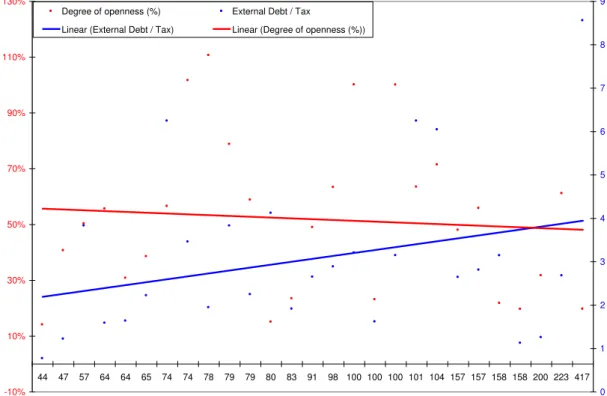
In order to estimate the e¤ect of the openness and debt levels over the past currency crises, we present in Figure 1 the currency depreciation3 observed versus
the degree of openness4 and versus the external debt related taxes for the selected
countries. We also present the best linear proxies for both relations. Looking to this plot, we can guess that in most open countries the devaluation required tends to be lesser, even without considering many other important variables in such an analysis. The following …gures present results of the model simulation which are detailed in section 3. They are divided into two blocks. In the …rst one we use Brazil as a benchmark economy to evaluate some qualitative results from the model, like the optimal …scal policy function; the crisis zone; how the degree of openness can a¤ect this zone and the devaluation-response; how much degree of openness is required to compensate the negative welfare e¤ect of more vulnerability (more risk premium and/or more external debt); what should be the shock required for the default to be better than the devaluation; and how the degree of openness a¤ects this requirement. In the second, we show aggregate results for all countries, verifying that our model can indicate, in a stylized way, the preferences for default-devaluation options and the magnitude of the currency depreciation required to overcome external crisis.
3We present details of these calculations and plot in the numerical exercise section and in the
Table 3. Note that only devaluations bigger than 30% are selected.
On a more methodological ground, the possibility that default can be welfare en-hancing is in accordance with the current bankruptcy literature, which says that it is optimal to have some bankruptcy in equilibrium, contrary to conventional wisdom (see Geanakoplos, Dubey and Shubik [12], for penalties on the utility function, and Araujo, Páscoa and Torres-Martínez [3], for in…nite horizon economies). Although, the risk of default should be kept under control. Accordingly, the introduction of lo-cal currency and tradable goods can give rise to the possibility of a better bankruptcy technology through devaluation of the local currency than just the repudiation of the external debt, which can be quite costly.
In the next section we describe the model and an equilibrium. Section 3 presents the numerical exercises and section 4 concludes them.
2
The Model with Tradable
The self-ful…lling debt crisis model of Cole and Kehoe ([7]) including debt denomi-nated in local currency is the basis to develop the model with trade. There is only one good in the economy produced with capital, k, inelastic labor supply and price normalized to one; three participants — national consumers, international bankers and the government; public external debt denominated in dollars or indexed to this currency, B , and public internal debt denominated in local currency, B. The ex-ternal public debt is only acquired by international bankers, and there is a positive probability of no rollover whenever its level is in the crisis zone. We consider that any suspension in its payment is permanent and total, as in the original model. On the other hand, public debt B is only taken up by national consumers, which are always prone to rolling it over, charging the price associated with the positive probability of partial repayment due to currency devaluation.
2.1
Uncertainty
We consider that the sunspot realization is conditional on realization. The probability that the international bankers’ con…dence is below the critical value is de…ned as , i.e. P ( ) = : If , is supposed to be distributed with uniform [0;1], but if > , is supposed to be one. The probability that the consumers’ con…dence is below the critical value given that international bankers are not willing to renew their loans is , i.e. P[ j ] = . Then, in the model with debt in local currency, the probability of a self-ful…lling external debt crisis occurring is (1 ), which is equal to[P ( )] [P( > j )]. In this case, there is a suspension of foreign credits and the price that the international bankers are willing to pay for the new dollar debt, q , is zero. The fear of default is self-ful…lling. With probability there is an external crisis, q = 0, but the government devalues its currency in order to avoid the default. In this case both national and foreign creditors have very low con…dence that the government will honor its debt obligations. Figure 2 sums up the three possible states in the crisis zone.
We rule out from the model the possibility that both default and devaluation can be used together. Instead, we consider that during a crisis each one of them can be used with some positive probability, given by sunspot, . These probabilities can be inferred from the spreads of the interest rates on local currency public debt and on dollar currency public debt over the free risk rate. The results presented in the numerical solution (Figure 7) show that for low levels of the external debt, devaluation is the best response in the crisis zone and, for high levels, default is preferable. We also assume that the commitment to no-devaluation (no-in‡ation) is enforceable when there is no external crisis (q >0). This way, devaluation can be used only to avoid default, when the economy is hit by a shock.
2.2
Crises responses and trade openness
The decision to default on the dollar debt is characterized by the government’s de-cision variable, z , being equal to zero from default decision on, or being otherwise equal to one. We assume that default causes a permanent fall in national produc-tivity, a, from 1 to , with (0;1). Meanwhile, the decision whether or not to devalue the local currency is described by the government decision variable, z, with
z (0;1]. On one hand, when international creditors do not renew their loans and the government chooses to default, the local-currency bond pays one good, z = 1, and the dollar bond pays nothing, z = 0. The productivity of the economy falls to . On the other hand, if the government decides for devaluation, then local-currency bond delivers goods,z = ;there is no default on the dollar debt,z = 1, and the productivity turns to be . The cost of devaluation is described by a permanent fall in productivity, a, from 1to , with (0;1]for all : Note that corresponds to the best in‡ation response against the crisis and conditional on z = 1:5 Therefore,
5We consider that this best-response is also permanent, i.e. if z
t = < 1 then zt+i =
devaluation of the local-currency also brings a cost in terms of lower productivity and a bene…t of extra revenue that helps to avoid an external default. Finally, pro-vided that there has not been either a default or an in‡ation tax, previously or at present, then a is equal to one and the government decision variables are z = 1
and z = 1. Figure 2 shows the three possible government decisions and implied productivity, depending on the realization of the sunspots and considering external debt in the crisis zone. The crisis zone is de…ned as the interval of the external debt for which the government prefers to default if (q = 0); and not to default if
(q > 0). Both equilibria are possible and the selected one is given by the sunspot variables.
Real devaluation
The international market is the place to settle dollar-denominated debt, while the domestic market is the one to settle local-currency obligations. The indebted country produces goods locally and pays the maturing external debt according to the price of the good exchanged abroad, which we call tradable. There is only one good but with di¤erent prices depending on the place it is traded. This trade could be thought of as occurring through an exchange rate market. The government budget constraint in each period (t), in units of the domestic goods, is given by:
gt :[atf(Kt) Kt] +T Bt Rt 1ztBt +RtqtBt+1 Btzt+Bt+1qt (1)
withg being the public expenditure, being the tax rate,f(:)6being the production
function, K is the capital stock of the economy,R is the amount of domestic goods per unit of tradable, is the depreciation factor, T Bt is the trade balance and q,
q are the prices of the local currency-denominated bond in unit of domestic goods and the dollar-denominated bond in units of tradable, respectively.
We suppose that every country’s international transaction occurs through the government budget constraint (1). This way, the imbalances in the current account,
( T Bt);plus the imbalances in the nonreserve capital account, Rt 1ztBt RtqtBt+1 ,
are compensated by o¢cial reserve transactions, which cause a reduction in the pub-lic expenditure(g). We also assume that the nominal exchange rate is …xed or pegged to another currency, but might su¤er a signi…cant devaluation after the realization of an external shock. National governments may choose to devalue the local-currency in order to make local goods cheaper, impacting the trade balance, T Bt, and the return of its debts. As long as the pass-through coe¢cient from nominal exchange rate to prices, ; is less than one, the devaluation is followed by a rise in the real exchange rate, R, and a rise in the domestic in‡ation, which implies that z is less than one, i.e. z = ( ). In this case, the government pays B to local investors, reducing the real return on the local-currency debt. Furthermore, the real devalu-ation increases the volume of exports and decreases the demand for both imports
Real e¤ects over local public debt return and real exchange rate is present in the …rst period after devaluation. From the second period on, in‡ation is predictable and a¤ects only nominal variables.
and new dollar debt. We consider that it does not increase the price to be paid for the old external debt as the government can pay it before changing R.
Then, the advantages of the devaluation-response embrace avoiding an external default, reducing the local-currency debt to GDP ratio; since B, instead of B, is settled from the moment of the devaluation on; and improving the trade balance. All these gains should be weighed up in terms of welfare. On the other hand, there are costs related to the in‡ation tax and to the rise in the value of the foreign obligations.
To compute such e¤ects in the trade balance, we consider that its value,T B(R);
depends on the real exchange rate. At times of no external crisis, R is equal to one and the trade balance enters as a constant term in the government budget constraint. We are only interested in the revenue that the government obtains from an improvement in the trade balance after a real devaluation, D(R)7. This
revenue depends on the intensity of the real devaluation, the trade volumes, and the real-exchange-rate elasticities of exports and imports, and , respectively8,
as developed in the Appendix. We set D(R) as
D(R) = (R 1) ( + R 1)Imp(1)
where (R 1) is the rate of devaluation, is the export-import ratio and Imp(1)
is the initial level of imports when R = 1. Then, a devaluation produces a positive change in the trade balance as long as( + R)is greater than one, which means that the trade account is improved when the response of export-import ratio to a change of the real exchange rate is preponderant. In this case, the more price-elastic the trade volumes are, the greater the improvement will be. Note that the devaluation also may worsen the trade account because of the negative wealth e¤ect on the import volumes ordered before the change in the real exchange rate.
2.3
Market participants
At any time t, the representative consumer maximizes the expected utility
max
fct;kt+1;bt+1gt
E
1
X
t=0
t
[ct+v(gt)]
subject to the budget constraint, given by
ct+kt+1 kt+qtbt+1 [at:f(kt) kt] (1 ) +bt bt(1 zt)
given k0 > 0 and b0 > 0. At time t; the consumer chooses how many goods to
save for the next period, kt+1, to consume at present, ct, and the amount of new
local-currency debt to buy, bt+1, which consists of zero-coupon bonds maturing in
one period. The utility has two parts: a linear function of private consumption,
ct, and a logarithmic function of government spending, v(gt) ln(gt). The right-hand side of the budget constraint corresponds to the sum of consumer’s income from production, after taxes and capital depreciation, plus the return on the local-currency debt acquired in the previous period. If there is no devaluation, zt equals to one and this return equals to bt domestic goods.
Analogously, at any timet, the problem of the representative international banker is
max
fxt;bt+1g t E 1 X t=0 txt
subject to the budget constraint
xt+Rtqtbt+1 x+Rt 1ztbt
given b0 > 0. At time t, the bankers choose how many goods to consume, xt, and the amount of new government bonds denominated in dollar to buy, bt+1. The expenditure on new government debt is Rtqtbt+1, where qt is the price of the
zero-coupon bond that pays one unit of tradable good at the maturity (t + 1) if the government does not default. The right-hand side includes the revenue received from the bonds purchased in the previous period,Rt 1ztbt;and the …xed endowment
‡ow,x. The decision variablez indicates whether the government defaults (z = 0) or not (z = 1). If it defaults, then the bankers receive nothing.
The government is assumed to be benevolent in the sense that it maximizes the welfare of national consumers, with no commitment to honor its obligations. Its budget constraint is given by (1), where the left-hand-side is the government’s consumption and the right-hand-side includes the following terms: the income tax, the trade balance and the interest paid both on the dollar debt and on the local-currency debt.
In order to obtain the real exchange rate as a function of the government in‡ation decision, we de…ne the real exchange rate devaluation as:
R R = E E + P P P P
Assuming that the foreign price levelP is constant, we obtain the local-in‡ation rate {:
P P = 1
R R
with the pass-through from nominal exchange rate change to local prices, ; being equal to P
P = E
E : The value of z; which corresponds to the units of domestic
goods that a local-currency bond actual pays at maturity, is de…ned as
z = 1 1 +{
Accordingly, we arrive at an expression that relates z to the change in the real exchange rate:
z = 1 + (R 1)
(1 )
1
(2)
where the devaluation rate is given by (R 1); since R0 = 1.
The government is assumed to behave strategically as it can foresee the optimal decisions of all market participants; including its own,zt, ztand gt; given the initial aggregate state of the economy and its choices ofBt+1andBt+1. To match aggregate
and individual variables it is assumed that, in the initial period, the supply of dollar debt B0 is equal to the demand for this debt, b0; the supply of local currency debt
B0 is equal to its demand, b0; and the aggregate capital stock per worker, K0, is
equal to the individual capital stock, k0. The population of both consumers and
bankers is continuous and normalized to unit.
2.4
A recursive equilibrium
The de…nition of a recursive equilibrium follows the same procedure developed by Cole and Kehoe ([7]). The actions of the participants are taken backwards according to the timing in each period.
Timing of actions within a period
the sunspot variables and are realized and the aggregate state of the economy is s (K, B , B, a 1, , );
the government, taking the dollar-bond price scheduleq =q (s,B 0) as given,
chooses the new dollar debt, B 0;
the government, taking the local-currency bond price schedule, q = q(s, B 0)
as given, chooses the new local-currency debt, B0;
international bankers, taking q and z as given, choose whether to purchase
B 0;
local investors, consideringq , q andz as given, decide whether to acquireB0;
the government decides whether or not to default on dollar debt, z ;
the government decides whether or not to devalue the local currency, z, and chooses its current consumption, g;
consumers, taking a(s; z ; z) as given, choose cand k0.
consumers who move last. For simplicity, from now on, we refer to consumers and government decisions as C and G;respectively9.
Each consumer knows the stock of capital saved, k, the stock of local-currency debt purchased,b, the aggregate state of the economys, and the new dollar and local-currency debts o¤ered by the government, B 0 and B0. Given s and B 0, consumers
take as given the price that international bankers are willing to pay for the new dollar debt, q (s; B 0), and the price that turns them indi¤erent to accepting or
not the new local-currency debt, q(s; B 0): They are also able to anticipate the
government’s decisions for the coming period, G(s0). Therefore, when consumers choose the amount of new local-currency debt, b0, their state is sc (k; b; s; G(s)).
The value function for the representative consumer is given by:
Vc(sc) = max
c;k0;b0fc+v(g) +EVc(s 0
c)g (3)
s:t: : c+k0 k+qb0 (1 ) [af(k) k] +zb ; ( c; k0)>0:
Each international banker decides how much public debtb 0 to buy, knowing the
amount of dollar debt purchased in the previous period, b , the aggregate state,
s, and the government’s decision G(s). They also take prices as given, q(s; B 0)
and q (s; B 0), and the government decisions for the coming period G(s0):
Accord-ingly, their state is sb (b ; s; G(s)) and their value function is de…ned by:
Vb(sb) = max
x;b 0 x+ EVb(s 0
b) (4)
s:t: : x+Rq b 0 x+R 1z b ; x 0
The subscript ( 1) indicates that when q = 0 and the government choose to
devalue, it can pay the old debt …rst.
Finally, the government makes decisions twice within a period. When it chooses its new debt levels, it knows the states. Moreover, it takes price schedulesq (s; B 0)
and q(s; B 0) as given, as well as its optimal choices induced by the new debts,
G(s0jB0; B 0). Likewise, the government also recognizes that it can a¤ect the optimal choices of consumers, C(sc), the price schedules q (s; B 0) and q(s; B 0), and the
productivity a(s; z ; z) of the economy.
Then, in the beginning of each period, the government chooses B 0 and B0, and
its value function is de…ned by
Vg(s) = max
B 0;B0 c(sc) +v(g) + EVg(s
0) (5)
s:t: : g =g(sg) ; z =z (sg) ; z =z(sg)
where the last three restrictions indicate that the government chooses the best ac-tions given its previous choices about the debt level. sg is de…ned as the state of the government, (s; B 0; B0). Therefore, after national and international investors
de-cide about buying new debt, the government dede-cides whether or not to default and
whether or not to devalue the local currency. By comparing welfare levels according to repayments decisions, and taking all debt levels as given, the policy functions
z (sg),z(sg)and g(sg), are solutions for:
max
z (s);z(s);gc(sc) +v(g) + EVg(s
0) (6)
subject to,
g+z R( 1)B +zB [a(s; z ; z)f(K) K] +T B(R) +q RB 0+qB0
g 0; z (0;1]
0 = (R 1) (1 z )
where the last restriction indicates that default and devaluation cannot be im-plemented at the same time. We de…ned z and z as function of s because when to default is better than not to default (z = 0 g z = 1jz = 1), then the actual
government response to the crisis, namely devaluation or default, depends on the sunspot- realization. We also consider that when devaluation is used to avoid the default, z is chosen to maximize the welfare conditional to z = 1:
De…nition of an equilibrium
An equilibrium is de…ned as a list of value functions Vc for the representative consumer,Vb for the representative international banker, andVg for the government; policy functions C for the consumer, b 0, for the international banker, andGfor the
government; price functions for the dollar debt, q , and for the local-currency debt,
q; and an equation for the aggregate capital motion, K0, as follows:
(i) given G; q; q ; Vc is the value function for the solution to the problem of the consumers (3), and C are their optimal choices;
(ii) given G; q; q ; Vb is the value function for the solution to the problem of the international bankers (4), and b 0 is their optimal choice;
(iii) given C; q; q ; Vg is the value function for the solution to the problem of the government (5 and 6) and G are its optimal choices;
(iv) B 0(s)2b 0(sb);
(vi) B0(s)2b0(sc);
2.5
Equilibrium Analysis
The behavior of consumers and bankers depends on their expectations regarding whether or not the government will default on the dollar debt or create in‡ation tax on the local-currency debt through devaluation. On the other hand, the government actions also depend on these expectations which have real e¤ects through the debt prices and investment levels.
When making their decisions about capital accumulation, consumers compute the expected productivity for the economy according to their beliefs about the pos-sibility of a crisis occurring in the next period, and to the pospos-sibility that this crisis results in a default or a currency devaluation. Then, the optimal capital accumula-tion, kt+1, depends on the consumers’ expectations about productivity,Et[at+1];as
follows:
1
= 1 + (1 ) [f0(kt+1)E(at+1) ]
Furthermore, consumers act competitively and are risk neutral, so they may pur-chase new public debt denominated in local-currency if its price equals the expected return to 1= :
1
= Et[zt+1]
qt
The more closed the economy is the greater is the devaluation (in‡ation) required during the crisis and the smaller is the expected value for zt+1: So, interpreting q1t
as being the interest factor over the local currency debt we can say that the interest rate is decreasing in the degree of openness.
Analogously, international bankers act competitively and are risk neutral, so they may purchase new public debt denominated in dollar-currency if its price equals the expected return to 1= :
1
= Et zt+1
qt
During a crisis (& < ) they are convinced about default on the next period and so they set qt = 0:
Finally, to complete the equilibrium analysis we must …nd which are the govern-ment actions. LettingVg(sjz; z ; q )denote the payo¤ to the government conditional on its decisions, z and z ;and conditional on the priceq ; and also considering that the public debt level denominated in the local currency cannot change over time
(Bt = Bo 8 t)10; it is possible to construct an equilibrium with the crisis zone
de…ned by the external debt level as in the Cole Kehoe model ([7]).
Next, we de…ne the participation condition which ensures that the government will want to honor the current external debt given it is able to sell new one:
10From now on we consider that this assumption holds. Otherwise, there would be no external
Vg(sj1;1; q >0)> Vg(sj1;0; q >0) (7) Analogously, we de…ne theno-lending condition which ensures that the govern-ment will want to default during a crisis:
Vg(sj1;0; q = 0)> Vg(sj1;1; q = 0) (8) The crisis zone is de…ned as the interval for the current external debt level,
(b; B]; where b is the greatest external debt level so as equation (8) does not hold with (b; kn) s; and B is the greatest external debt level so as equation (7) holds for B; k s: When the economy is out of the crisis zone, i.e. B b; there is always external credit available. Since the bankers know that the government would not to default even if the price were zero, they do not refuse to rollover new bonds. In the crisis zone the bankers are aware of the possibility of default, and may refuse to sell new bonds (q = 0). In this case, default is desirable, but with probability the government devalues to avoid the default.
Although we do not compare the payo¤s of devaluationversus default to charac-terize the crisis zone (we maintain the possibility of both responses occur), we com-pute in the numerical exercises, presented in the next section, the level of external debt,eb, for which government would be indi¤erent between default and devaluation. We also verify thateb (b; B) and that devaluation is the best response in the crisis zone if B <eb: IfB >eb; default is the best response in the crisis zone.
Table 1 presents the four possible equilibrium capital accumulation and prices, according to the expectations. In the …rst line of the table we consider that the external debt is out of the crisis zone. In the second one we consider that the external debt level is in the crisis zone and the two last present the values for the after-crisis economy. Each one of the three last lines corresponds to the three states characterized in Figure 2.
3
Numerical Exercises
In this section, we …rst present numerical exercises for the Brazilian economy to show some qualitative results from the model. Secondly, we present aggregate results for 58 currency crises and attempt to outline some of the factors that make countries adopt di¤erent crisis responses, with more or less devaluation, and choosing default or not.
3.1
Qualitative results
98-99. The government discount factor, , is approximated by the yearly yield on government bond issued by the US, whose values were about 5 percent. Based on these …gures, we interpret a period length as being one year and a yearly yield on risk free bonds, r; as being 0:05; which implies a discount factor of 0:95(= (1 +r) 1). The choice of the functional forms for v(:) and f(:) were the same used by Cole and Kehoe [7], that is, v(g) = ln(g) and f(k) = Ak where capital share is es-tablished at 0:4 and the scale factor at10. The parameter equals 0:95; assuming that default causes a permanent drop in productivity of 0:05. For z = ; the cor-respondent in‡ation rate is (1 )= ; which implies the welfare cost of in‡ation,
;estimated according to Simonsen and Cysne11 ([10]). The probability of default,
(1 ), and the probability of in‡ation, ( ), are calculated on the basis of the risk premium practiced in the …nancial market according to the following expression:
1
= 1 +rDBR (1 (1 )) = 1 +r BR
LC (1 ( ) (1 ))
where rBR
D and rLCBR are yearly yields on Brazilian public debt denominated,
respec-tively, in dollar and in local currency (discounting the expected in‡ation of Brazilian currency), and is given by the unexpected yearly in‡ation associated with deval-uation.
Data forrBR
D are available for the period of analysis, whilerBRLC only since January
2002, when its value was about0:1212. Therefore, considering the values for ; rBR D ;
and rBR
LC equals to0:5; 0:14;and 0:12, respectively, we can compute ( ; )as being
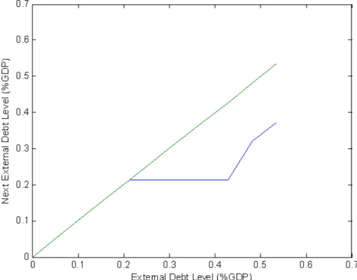
equal to (0:2;0:61). In Table 2 we present the values of parameters and variables used in the simulations for the Brazilian economy, whose results are described next. Figure 3 shows that when the external public debt is in the crisis zone the optimal policy is to move out from it. But it may be di¢cult to reduce public expenditure and Figure 4 shows that an alternative policy could be lengthening the maturity13.
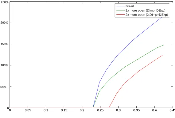
These conclusions remain the same as in the original model. Figures 5, 6, and 7 present the e¤ects of the degree of openness over the economy. As shown in Figure 5, if the economy has its imports and exports enlarged without changing the trade balance, i.e. the gains in the volume of exports (Dexp) equal the gains in the volume of imports (Dimp), then only the cap of the crisis zone becomes greater. But if the economy can improve its trade technology and enlarge exports faster than imports, then the international capital in‡ow becomes greater and both the ‡oor and the cap increases. In …gure 6 it is possible to see that, according to the model, the
11In the estimation of welfare cost of in‡ation we use Bailey’s approximation and the money
demand speci…ed as kr a; where r is the logarithmic annual in‡ation (see Simonsen and Cysne
[10]). We setkand aequals to0:07and0:6;respectively.
12Yearly yield on LTN minus expected in‡ation.
13We follow Cole and Kehoe approach for “lengthening the maturity structure”. Henceforth,
lengthening the maturity structure means converting an initial quantity B of one-period (one
year) bonds into equal quantitiesBn of bonds of maturityn (1,2,. . . ,N). Then, the government
redeemsBn bonds every period and sellsBn n-period bonds, whereBn(1 qn) =B (1 q );and
qn= n
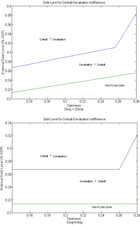
devaluation required to response to a crisis is increasing in the external debt level and decreasing in the degree of openness. Figure 7 also shows that the “devaluation– better-than-default” region is increasing in the degree of openness. Finally, …gures 8, 9, and 10 correspond to welfare analyses. They show how much debt must be paid to compensate the welfare loss related to an increase in the external risk, and how much improvement in the trade is required to compensate the welfare loss related to an increase in both the external risk and the external debt. Note that in Figure 10 both expected welfare and welfare after crisis are considered.
3.2
Comparative results
The parameters used in the simulations for the other countries are presented in Table 3. To compare results across countries we change only a few parameters which we consider more relevant to explain di¤erences between economies and their responses to crisis. The variables that are not presented in Table 3 are the same for all countries including Brazil (Table 2).
Figure 11 shows that, according to the assumptions of our model, the “countries on the left side” were more prone to choosing default than the “ones on the right”. Results match 85%of the crises with “reality” in predicting that default is the best response whenever it actually occurs and it is not the best response whenever it does not occur. Red marks show where the model failed.
Figure 12 presents the estimated devaluations for di¤erent pass-through values. Note that the results are quite similar to a wide range of this parameter. Devaluation rates change signi…cantly only when considering that pass-through is very close to one.
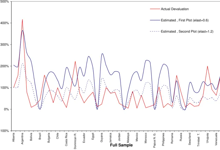
Figure 13 compares actual devaluations and those predicted by the model. In the …rst plot the elasticities ( ; ) of 0:6 were considered, and in the second plot we double this value. Note that for greater elasticity less devaluation is required to overcome the external crisis as expected. Accordingly, most devaluations predicted are overestimated, but not too far from reality. Moreover, we do not consider that our numerical exercise is a good predictor for actual devaluation, since we have made simpli…cations to compute after-crisis payo¤s as considering zt+i = 0; zt+i = for
alli >0;respectively, in default and devaluation responses. Our aim is to outline the di¤erent crisis responses adopted by countries considering factors as the degree of openness, debt levels in both currencies, taxes, and risk-premiums. In this sense, we are more interested in comparing the shape of predicted versus actual devaluations plots.
Figure 14 replicates Figure 13 excluding the devaluations lesser than 30% and separating countries that experienced default from the others.
six months for all crises. The new level of the exchange rate is considered as the mean of the exchange rate for this crisis period and the actual devaluation for each country is computed as from the exchange rate level immediately before the crisis period.
4
Conclusions
References
[1] Araujo, Aloisio and Marcia Leon, 2002, Ataques Especulativos sobre Dívidas e Dolarização, Revista Brasileira de Economia, 56:1, 7-46.
[2] Araujo, Aloisio; Leon, Marcia; and Rafael Santos. Monetary Arrangements for Emerging Economies. 2006.
[3] Araujo, Aloisio; Páscoa, Mário and Juan P. Torres-Martínez, 2002, Collateral Avoids Ponzi Schemes in Incomplete Markets, Econometrica, 70:4, 1613-1638.
[4] Calvo, Guillermo. The case for Hard Pegs. Unpublished manuscript, University of Maryland. Mimeographed.
[5] Calvo, Guillermo; Izquierdo, Alexandre; and Talvi, Ernesto. Sudden Stops, the Real Exchange Rate, and Fiscal Sustainability: Argentina’s Lessons. NBER Working Paper No. 9828. July 2003.
[6] Chang, R.; Velasco, A.;2000 . Exchange rate policies for developing countries. American association papers and proceedings 90 (May): 71-75.
[7] Cole, Harold and Timothy Kehoe, 1996, A self-ful…lling model of Mexico’s 1994-1995 debt crises, Journal of International Economics, 41, 309-330.
[8] ——–, 1998, Self-Ful…lling Debt crises, Federal Reserve Bank of Minneapolis, Sta¤ Report, 211.
[9] ——–, 2000, Self-ful…lling Debt crises, Review of Economic Studies, 67:1, 91-116.
[10] Cysne, Rubens and Mario Simonsen, 1994, Welfare Costs of In‡ation: The Case for Interest-Bearing Money and Empirical Estimates for Brazil, Ensaios Econômicos, 245.
[11] Dornbush, R.; 2000. Millenium Resolution: No more funny money, Financial Times, January 3.
[12] Dubey, P.; Geanakoplos, J.; and Shubik, M. (2005): “Default and Punishment in General Equilibrium” Econometrica, 73(1).
[13] Frankel, J.;1999. No single currency regime is right for all countries or at all times. W.P. n 7338, National Bureau of Exonomic Research, Cambridge, Mass.
[14] Hausmann, R.; 1999. Should there be …ve currencies or one hundred and …ve? Foreign Policy 116: 65-79.
[16] Mussa, M.; Masson, P.; Swoboda A.; Jadresic, E.; Mauro, P.; Berg, A.; 2000. Exchange rate regimes in an increasingly Integrated world economy. Washing-ton,D.C.:International Monetary Fund.
[17] Paiva, Claudio. Trade Elasticities and Market Expectations in Brazil. IMF Working Paper, WP/03/140, Jul. 2003.
[18] Reinhart, C.; Rogo¤, K; Savastano, M.. Debt Intolerance. NBER Working Pa-per No 9908. August 2003.
5
Figures and Tables
-10% 10% 30% 50% 70% 90% 110% 130%
44 47 57 64 64 65 74 74 78 79 79 80 83 91 98 100 100 100 101 104 157 157 158 158 200 223 417
Devaluation (>30%)
0 1 2 3 4 5 6 7 8 9
Degree of openness (%) External Debt / Tax
Linear (External Debt / Tax) Linear (Degree of openness (%))
Figure 1: Currency Crisis, Degree of Openness and External Debt
Figure 4: Crisis Zone - Brazil
0 0.05 0.1 0.15 0.2 0.25 0.3 0.35 0.4 0.45 0
0.5 1 1.5 2 2.5
Brazil
2x more open (DImp=DExp) 2x more open (2.DImp=DExp)
100% 150% 200%
50% 250%
0 0.05 0.1 0.15 0.2 0.25 0.3 0.35 0.4 0.45
0 0.5 1 1.5 2 2.5
Brazil
2x more open (DImp=DExp) 2x more open (2.DImp=DExp)
100% 150% 200%
50% 250%
0 2 4 6 8 10 Guyana Egypt Morocco Morocco Bolivia Philippines Costa Rica Ecuador Albania Chile Argentina Mexico Ecuador Russia Chile Venezuela Paraguay Uruguay Chile Jamaica Jordan Bulgaria Trinidad T. Venezuela Jamaica Honduras Brazil Egypt Argentina Russia Romania Philippines Swaziland Papua N. G. Costa Rica Mexico Venezuela Thailand Malasya Turkey Argentina Gabon Botswana Dominican R. def
ault > devaluation
def
ault < devaluation
(Act
ual Exter
nal Public Debt
0%
100% 200% 300% 400%
Albania Argentina Argentina Argentina Bolivia Botswana Brazil Brazil Bulgaria Chile Chile Chile Costa Rica Costa Rica Dominican R. Ecuador Ecuador Egypt Egypt Gabon Guyana Honduras Jamaica Jamaica Jordan Korea Malasya Mexico Mexico Mexico Morocco Morocco
Papua N. G.
Paraguay Philippines Philippines Romania Russia Russia Singapore Swaziland Thailand
Trinidad T.
Full Sample -100% 0% 100% 200% 300% 400% 500% Albania Argent ina Bolivia Brazil Bulgar ia Chile Co sta R ica Domini can R. Ec uador Egy pt Guyana Jama ica Jordan Mal asya Me xic o Mor occ o Pap ua N. G. Philippin es Romania Ru ssia Swaz iland Trini da
d T.
Uruguay
Ven
ez
uela
Actual Devaluation
Estimated , First Plot (elast=0.6)
Estimated , Second Plot (elast=1.2)
Devaluations (>30%) 0% 100% 200% 300% 400% 500% 600% 700% Brazil Tur key Me xi co Jamaica Eg ypt Argentin a Ho ndur as Ven ez uela Brazil Argentin a Ch ile Eg ypt Ven ez uela Ecuad or
Jamaica Russia Me
xi co Ven ez uela Co sta Ri ca Bulgaria Ch ile Albania Para guay Russia Argentin a Ur ugua y Do min ican R. Actual Estimated default no default
Figure 14: Actual Devaluation Versus Estimated Devaluation (Restricted Sample)
Table 1: Equilibrium Prices and Investment
k0(E(at+1)) q(Ez) = q (Ez ) =
kn(1)
k + (1 ) + (1 ) :f1 [1 ]g f1 [1 ]g
k :
Table 2: Brazil(98)-Before Exchange Rate Devaluation
Length of Public Debt (Years) 1
Debt Relative to GDP %
Total Public Debt - B+B 53
External (Public) Debt - B 23
Local Currency (Public) Debt - B 30
Flow Relative to GDP %
Exports 7
Imports 7
Trade Balance - TB 0
Financial Cap.-Out‡ow -B (1 q ) 3
Investment - k0 k(1 ) 16
Private Consumption -c 59
Public Expenditure -g 22
Interest Rate - Local Debt - B(1 q) 2
Tax - 30
Parameters
-0:9524
f(k) = Ak and 10:k0:4 and 0:05
0:05 0:35
1 a
1 akln(1 +{( ))
(1 a)
0:6 0:6 0:61 0:20
Table3 : Selected Countries
Albania 1992 7 y 1992 100 11 89 21 67 0 5 15 30 25 y
Argentina 1990 12 n 80 10 5 10 43 17 6 6 87 92 y
Argentina 1989 11 n 417 13 7 10 83 40 3 66 95 90 y Argentina 2001 12 y 2001 158 12 10 12 39 16 5 5 78 15 n Bolivia 1989 7 y 1988 9 22 23 13 83 4 5 40 67 16 n Botswana 1975 7 n 1976 20 44 64 30 39 19 3 3 49 94 y
Brazil 1998 12 n 44 7 7 30 23 30 5 20 61 24 n
Brazil 1993 6 n 1992 158 11 9 26 29 62 5 9 94 96 y Bulgaria 1992 12 y 1992 100 47 53 36 114 115 12 55 65 90 y Chile 1984 8 y 1985 30 24 25 29 69 25 5 31 75 26 n Chile 1982 5 y 1983 47 19 21 29 35 4 8 30 60 26 n Chile 1971 12 y 1972 100 11 12 15 25 21 8 37 67 12 n Costa Rica 1987 8 y 1987 8 32 36 21 98 18 5 19 90 25 n Costa Rica 1980 12 y 1981 98 26 37 17 48 28 8 7 33 82 y Dominican R. 1984 12 y 1982 223 28 33 11 29 19 9 85 60 80 y Ecuador 1982 4 y 1982 29 22 24 11 44 0 3 37 65 18 n Ecuador 1999 9 y 1999 74 32 25 14 88 9 7 15 76 30 n
Egypt 1978 12 n 79 22 37 38 86 62 8 13 60 90 y
Egypt 1989 7 y 1987 57 18 32 29 112 74 7 8 93 8 n Gabon 1980 9 y 1978 12 65 32 36 35 4 14 23 50 77 n Guyana 1983 12 y 1982 24 46 65 43 255 193 6 16 60 10 n
Honduras 1990 2 n 101 29 34 15 93 16 8 4 84 89 y
Jamaica 1983 10 n 79 36 43 25 94 54 6 13 67 90 y
Jamaica 1991 8 y 1990 74 50 51 32 111 0 7 6 88 82 n Jordan 1988 8 y 1989 27 45 67 14 98 52 3 16 25 73 y
Korea 1997 6 n 15 35 36 17 11 1 8 10 67 41 n
Malasya 1985 12 n 5 54 49 27 54 30 8 4 73 112 y
Mexico 1989 1 n 5 20 19 13 51 27 5 6 74 92 y
Mexico 1994 11 n 65 17 22 13 29 8 4 18 70 86 y
Mexico 1982 2 y 1982 83 10 13 14 27 29 9 3 87 11 n Morocco 1984 11 y 1985 7 24 34 24 108 32 7 7 52 16 n Morocco 1983 7 y 1983 13 21 30 25 92 35 5 15 61 16 n Papua N. G. 1994 8 n 22 56 38 23 36 16 9 5 35 56 n Paraguay 1989 2 y 1987 104 34 37 10 59 2 5 22 66 38 n Philippines 1986 1 y 1986 8 24 22 12 78 16 3 25 54 20 n Philippines 1983 9 y 1983 27 22 28 12 63 18 8 4 85 83 y
Romania 1996 1 n 13 28 33 30 20 24 8 6 83 26 n
Russia 1992 12 y 1991 78 62 48 16 31 14 8 72 75 35 n Russia 1998 7 y 1998 157 31 25 20 57 29 5 60 62 26 n Singapore 1997 7 n 10 131 139 40 17 59 8 3 66 52 n
Swaziland 1985 7 n 28 57 85 29 64 1 6 21 59 88 y
Thailand 1997 3 n 14 48 47 18 41 0 8 4 27 81 n
Trinidad T. 1988 7 y 1989 17 39 34 29 47 17 5 19 78 40 n
Turkey 2001 1 n 64 24 32 28 45 27 5 4 75 96 y
Uruguay 1982 11 y 1983 200 14 17 21 27 18 7 5 79 19 n
Venezuela 1989 2 n 157 20 27 19 51 5 4 3 67 92 y
Venezuela 1984 1 y 1982 64 20 11 22 36 0 3 19 58 33 n Venezuela 1995 11 y 1995 91 27 22 16 43 24 8 25 79 23 n
TAX/GDP (%)
B*/GDP
(%) 3
bind/GDP
(%)2 Actual devaluation (%) EXP/GDP (%) Currency Crises
Start of Episode(y/m)
Debt Default1 ?
To reach comparative results, we set scale factor (A) equals to 15 for all countries, including Brazil. 1: Default or restructuring of the external debt. Many episodes lasted several years. 2: bindis the debt for default-devaluation indifference, and its value split the crisis zone into two. 3: Only to compute the critical
debt levels avoiding empty crises zones, in some countries, we consider that government has constant endowment of 0.75 GDP/year. (n) means no endowment and (y) means 0.75-endowment.
Sources:The World Debt Tables, World Bank Book ; International Financial Statistics, Yearbook / IMF ; World Development Indicators, The World Bank ; Country Info Base free available in http://www.dbresearch.de ; Central Banks.
B/GDP (%)
Free risk
rate (%) π*(%)π (%) IMP/GDP
(%) Country
6
E¤ect of Real Devaluation on the Trade Balance
De…ning Exp as exports measured in domestic output units, Imp as imports de-nominated in units of tradable, R1 as the initial real exchange rate, and R2 as its
new level after devaluation, we can compute the trade balance change D(:) as:
T B(R) = Exp(R) Imp(R)R T B
R =
Exp R
Imp
R R2 Imp(R1) T B
R =
Exp R
R1
Exp(R1)
Exp(R1)
R1
Imp R
R1
Imp(R1)
R2
Imp(R1)
R1
Imp(R1)
T B
R =
Exp(R1)
R1 Imp(R1)
+ R2
R1
1 Imp(R1)
Where = ExpR R1
Exp(R1) and =
Imp R
R1
Imp(R1): De…ning as the exports-imports
ratio, R1 1; and R2 R, we obtain