Statistical Distributions of Discrete Walsh Hadamard Transform Coefficients of Natural Images

Vijay Kumar Nath and Deepika Hazarika

Department of Electronics and Communication Engineering, School of Engineering, Tezpur University (A Central University), Napaam, Tezpur, Assam, India.

vknath@tezu.ernet.in and deepika@tezu.ernet.in

A

For low bit rate applications, the discrete Walsh Hadamard transform (WHT) shows almost comparable results when compared to the popular discrete Cosine transform (DCT) in terms of compression efficiency, peak signal to noise ratio (PSNR) and visual results. The discrete WHT is a best choice which compromises between the computational complexity and compression efficiency. The great advantage of the discrete WHT is its relatively very low computational complexity when compared to DCT. However there is no definitive study reported in literature regarding the statistical distributions of discrete WHT coefficients of natural images. This study performs aχ2 goodness of fit test to determine the distribution that best fits the discrete WHT coefficients. The simulation results show that the distribution of a majority of the significant AC coefficients can be modelled by the Generalized Gaussian distribution. The knowledge of the appropriate distribution helps in design of optimal quantizers that may lead to minimum distortion and hence achieve optimal coding efficiency.

K

Image Compression, Discrete WHT, _χ2

test, Statistical analysis

1.

I

DCT [1] has been very popularly used in many image and video coding standards like JPEG, MPEG1, MPEG2, H.261 [2,3]. But the computational complexity of the DCT is relatively very high which may not be preferred in several real time applications.

The discrete WHT [4,5,6,18] is a orthogonal non sinusoidal transform which shows almost comparable performance in image compression applications when compared to DCT. The discrete WHT is popular for its very low computational complexity. The discrete WHT is considered as the best option whenever there is a compromise between the energy compaction capability and computational complexity. However till now, no study has been reported in the literature, on the distribution of discrete WHT coefficients of the natural images. In contrast, there is a huge amount of studies reported in the literature dealing with the distributions of 2D DCT coefficients of natural images [7,8,9,10].

the coefficients are lumped into one density function, the Cauchy distribution provides the best fit. In [9], Muller found that the Generalized Gaussian distribution best approximates the statistics of the 2D DCT coefficients. Smoot and Reeve [19] study the statistics of the DCT coefficients of the differential signal obtained after motion estimation.

They observe that the statistics are best approximated by the Laplacian distribution.

In this paper, considering Gaussian, Laplacian, Gamma, Generalized Gaussian and Cauchy distributions as probable models [11,12], we study the statistical distribution using χ2 _Goodness of Fit test [13]. The model distribution that gives the minimum χ2statistic is chosen as the best fit. The χ2test of fitshowed that Generalized Gaussian distribution best models the statistics of discrete WHT coefficients of natural images. These results can be used to design optimal quantizers for discrete WHT coefficients. The organization of the paper is as follows. Section 2 provides the introduction to discrete WHT. 2

χ Goodness of Fit test is explained in Section 3. Section 4 describes the model statistical distributions. Experimental results are presented in Section 5 and the paper is concluded in Section 6.

2.

The basis functions of discrete WHT [4] are not sinusoids unlike Fourier and Cosine transforms. The basis functions are based on rectangular waveforms with peaks of ±1. The N-point 1-D discrete Walsh Hadamard transform of a signal ( )x n is given as

1

0 1

( ) ( ) ( )

N

z m

V z x m y m

N

−

=

= , z=0,1,...,N−1 (1)

where y mz( )is the Walsh function of order zand is defined recursively as: y mz( )=0 for m<0and m>N−1

y m₀( ) 1= for m=0,1...,N−1 ₂ ( ) (2 ) ( 1)z (2 1)

z z z

y m =y m + − y m−

_{2 1}( ) (2 ) ( 1)z (2 1)

z z z

y + m =y m − − y m−

for z=0,1...N−1.

3

.

χ

2

χ and KS test [13] are the widely used goodness of fit test. The KS goodness of fit test statistic is a distance measure between the empirical cumulative distribution function (CDF) for a given data set and the given model cumulative distribution function. In contrast to the KS test, the 2

χ goodness of fit test compares the model probability density functions with the empirical data and finds out the distortion by the following equation

2 2

1

( )

e

k

i i

i i

O E

E

χ

= −

= (2)

where the range of data is partitioned into k_e disjoint and exhaustive bins B_i, i=1, 2,3,...,k_e.

i c i

E =n p is the expected frequency in bin Bi where pi=P x( ∈Bi) and Oi is the observed

frequency in bin Bi. ncis the total number of data samples. The model probability density

function which gives the minimum χ2 value can be considered as the best fit.

4.

We use 2

χ goodness of fit tests considering Gaussian, Laplacian, Gamma, Cauchy and Generalized Gaussian distributions [11,12] as probable models as these distributions are commonly used for statistical modeling of DCT coefficients. The parameters of the distributions were found using the maximum likelihood (ML) method.

4.1. Gaussian Probability Density Function The Gaussian probability density function is given by

2 2

1 ( )

( ) exp

2 2

X

x

f x µ

σ πσ

−

= − (3)

where µ is the mean and σ2 is the variance. The ML estimates of µand σ2are given by

1 1 n i i x n µ =

= (4)

2 2 1 1 ( ) n i i x n σ µ =

= − (5)

4.2. Laplacian Probability Density Function The Laplacian probability density function is given by

( ) 1 exp 2 X x f x a a µ −

= − (6)

where µ is the mean and a is the scale parameter. The variance is given by 2a2. The ML estimate of the parameter a is given by

1 1 N i i a x

N = µ

= − (7)

where µis estimated using (4).

4.3. Gamma Probability Density Function

The Gamma probability density function is given by [14]

4 ₃

3

( ) exp

2 8 X x f x x µ σ πσ µ − = −

− (8)

The parameters µ and σ are estimated using (4) and (5) respectively.

4.4. Generalized Gaussian Probability Density Function

The Generalized Gaussian probability density function [11,12,15] is given by

( ) exp 1 2 X x f x β β α α β = − Γ (9)

where Γ

( )

( )

0 , 0

t z

z ∞e t− −dt z

Γ = >

The shape parameterβis the solution of the equation 1 1 1 1 log log 1 0 N N i i i i i N i i x x x N x β β β β ψ β β β = = =

+ − + = (10)

where ψ

( )

_{( )}

( )

( )

z z

z

ψ =Γ′

Γ

The ML estimate ofα(for known ML estimate β) is given by

1 1 N i i x N β β β α =

= (11)

where N is number of observations.

Theβis determined using the Newton Raphson iterative procedure with the initial guess from the moment based method described in [16].

4.4. Cauchy Probability Density Function

The Cauchy probability density function [11,12,17] is given by

(

)

− + (12)

where x0is the location parameter and γis the scale parameter. For the Cauchy distribution with sample size N, the likelihood function L x

(

)

(

)

(

)

{

}

1 0 ₂

1 0 1 ,... ; , 1 / N N i i

L x x x

x x

γ

πγ γ

= = ∏

+ − (13)

The logarithm of the likelihood is given by

2 0 1

log log log log 1

N

i i

x x

L N π N γ

γ =

−

= − − − + (14)

Maximizing the log likelihood function with respect to y0and γgives:

2 0 0 1 1 0 N i i i

x x x x

γ γ

=

− −

+ = (15)

1 2 0 1 1 0 2 N i i

x x N

γ −

=

−

+ − = (16)

We use Newton Raphson iterative procedure to solve (15) and (16) for x0and γ. The median is used as an initial value for x0as described in [17].

5.

The 2

provides the minimum 2

χ statistic is considered to be the best fit under the 2

χ criterion. The nine AC coefficients C10, C11, C01, C20, C02, C12, C21, C03 and C30 used in the experiments were chosen because they usually have the most effect on the image quality.

Table 1. 2

χ statistics for a few discrete WHT coefficients of Lena (512x512) image

Coefficient Gaussian Laplacian Gamma Gen. Gaussian Cauchy

10

C 5.94x108 8165 87 32 115

11

C 4.36x108 5740 103 22 205

01

C 4.61x107 954 60 43 296

20

C 4.23x107 2216 55 45 130

02

C 1.02x106 639 36 106 333

12

C 1.25x106 1071 42 27 134

21

C 1.42x106 1156 25 45 176

03

C 6.38x106 4292 168 88 163

30

C 1.61x1012 20136 141 42 88

Table 2. χ2 statistics for a few discrete WHT coefficients of Barbara (512x512) image

Coefficient Gaussian Laplacian Gamma Gen. Gaussian Cauchy

10

C 1.00x1010 3184 49 39 126

11

C 1.12x109 2060 14 18 162

01

C 1.47x104 365 35 22 274

20

C 5.48x104 200 122 21 196

02

C 1.53x108 380 30 9 197

12

C 1.67x106 1811 28 26 183

21

C 2.04x107 223 69 19 245

03

C 1.00x105 543 19 64 242

30

C 2.59x105 16608 34 8 147

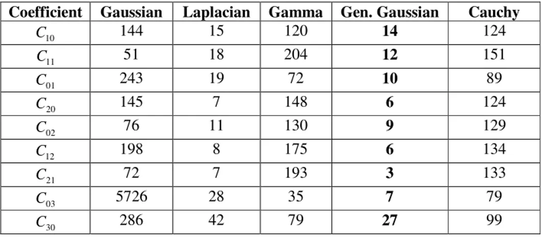
Table 3. _χ2

statistics for a few discrete WHT coefficients of Aerial (256x256) image

Coefficient Gaussian Laplacian Gamma Gen. Gaussian Cauchy

10

C 144 15 120 14 124

11

C 51 18 204 12 151

01

C 243 19 72 10 89

20

C 145 7 148 6 124

02

C 76 11 130 9 129

12

C 198 8 175 6 134

21

C 72 7 193 3 133

03

C 5726 28 35 7 79

30

Table 4. 2

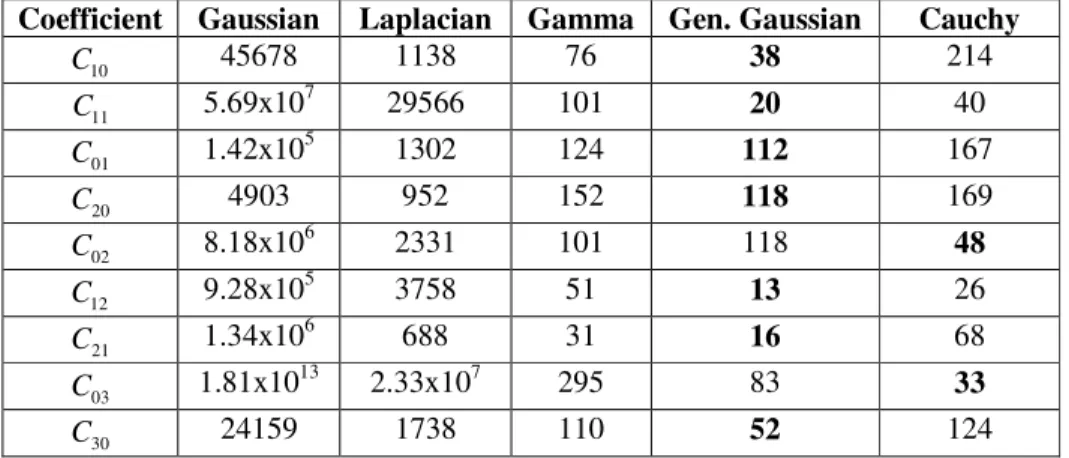
χ statistics for a few discrete WHT coefficients of House (256x256) image

Coefficient Gaussian Laplacian Gamma Gen. Gaussian Cauchy

10

C 45678 1138 76 38 214

11

C 5.69x107 29566 101 20 40

01

C 1.42x105 1302 124 112 167

20

C 4903 952 152 118 169

02

C 8.18x106 2331 101 118 48

12

C 9.28x105 3758 51 13 26

21

C 1.34x106 688 31 16 68

03

C 1.81x1013 2.33x107 295 83 33

30

C 24159 1738 110 52 124

Table 5. χ2 statistics for a few discrete WHT coefficients of Boats (512x512) image

Coefficient Gaussian Laplacian Gamma Gen. Gaussian Cauchy

10

C 2.19x105 741 43 17 142

11

C 8.60x104 636 65 12 143

01

C 7.48x108 3289 47 34 140

20

C 2.68x108 384 48 25 202

02

C 1.39x1010 1551 66 33 155

12

C 1.15x107 698 13 5 171

21

C 6.81x105 450 14 23 189

03

C 1.91x1013 6.14x104 128 13 146

30

C 54037 432 21 36 312

Table 6. 2

χ statistics for a few discrete WHT coefficients of Mandrill (512x512) image

Coefficient Gaussian Laplacian Gamma Gen. Gaussian Cauchy

10

C 1774 21 388 23 398

11

C 781 6 248 5 415

01

C 15427 35 573 40 462

20

C 843 72 110 43 330

02

C 12848 15 329 20 421

12

C 2.31x105 4 288 2 369

21

C 1317 43 234 24 364

03

C 23950 7 352 6 407

30

C 2925 79 163 18 311

If N xM is the size of the image after computation of 2D discrete WHT, then each coefficient

will have 8 N

x 8 M

values for the image to be used in KS and 2

χ test. Table 1, 2, 3, 4, 5 and 6

show the 2

General Gaussian distribution for most of the tested coefficients of all the images. Fig. 1 shows the empirical pdf of the discrete WHT coefficients along with the fitted Gaussian, Laplacian, Gamma, Generalized Gaussian and Cauchy pdfs. From Fig. 1 as well as from the values of the

2

χ statistic, it is clear that the Generalized Gaussian distribution provides a better fit to the empirical distribution then that achieved by the Gaussian, Laplacian, Gamma and Cauchy pdfs.

6.

In this paper, we perform theχ2goodness of fit tests to determine an appropriate statistical distribution that best models the discrete WHT coefficients of images. The simulation results indicate that no single distribution can be used to model the distributions of all AC coefficients for all natural images. However the distribution of a majority of the significant AC coefficients can be approximated by the Generalized Gaussian distribution. The knowledge of the statistical distribution of transform coefficients is very important in the design of optimal quantizer that may lead to minimum distortion and hence achieve optimal coding efficiency.

R

[1] N. Ahmad, T. Natarajan, and K. Rao, “Discrete Cosine Transform,” IEEE transactions on Computers, vol. C-23, no. 1, pp. 90-93, 1974.

[2] V. Bhaskaran and K. Konstantinides, Image and Video compression standards - Algorithms and architectures, Kluwer Academic Publishers, 1997.

[3] W. B. Pennebaker and J. L. Mitchell, JPEG still image data compression standard, New York: Van Nostrand Reinhold, 1992.

[4] A. K. Jain, Fundamental of Digital Image Processing. Englewoods Cliffs, NJ : Prentice Hall, 1989. [5] R. Costantini, J. Bracamonte, G. Ramponi, J. Nagel, M. Ansorge and F. Pellandini, “A low complexity video coder based on discrete Walsh Hadamard transform”, In EUPSICO 2000 : European signal processing conference, pages 1217–1220, 2000.

[6] A. Aung, Boon Poh Ng, C. T. Shwe, “A new transform for document image compression”, in Proc. of 7th International Conference on Information, Communications and Signal Processing, 2009.

[7] R. C. Reininger and J. D. Gibson, “Distributions of the two dimensional dct coefficients for images,” IEEE Transactions on Communications, Vol. 31, No. 6, pp. 835-839, 1983.

[8] J. D. Eggerton and M. D. Srinath, “Statistical distributions of image DCT coefficients," Computer Electrical Engineering, vol. 12, pp. 137- 145, 1986.

[9] F. Muller, “Distribution shape of two dimensional DCT coefficients of natural images,” Electronics Letters, vol. 29, no. 22, pp. 1935-1936, 1993.

[10] R. L. Joshi and T. R. Fischer, “Comparison of Generalized Gaussian and Laplacian modeling in DCT image coding,” IEEE Signal Processing Letters, vol. 2, no. 5, pp. 81-82, 1995.

[11] N. L. Johnson, S. Kotz, N. Balakrishnan: Continuous Univariate Distributions John Wiley and Sons ,1994 , Vol.1, 1st edition.

[12] N. L. Johnson, S. Kotz, N. Balakrishnan: Continuous Univariate Distributions John Wiley and Sons ,1994 , Vol.2, 2nd edition.

[13] V. K. Rohatgi and A. K. E. Saleh, An Introduction to Probability and Statistics, John Wiley and Sons, 2001.

[14] N. S. Jayant and P. Noll, Digital Coding of waveforms. Prentice Hall, 1984.

[15] S. Mallat, “A theory for Multiresolution signal decomposition: The wavelet representation,” IEEE Transactions on Pattern Recognition Machine Intelligence, vol. 11, pp. 674-693, 1989.

[16] K. Sharifi and A. Leon-Garcia, “Estimation of shape parameter for Generalized Gaussian distributions in subband decompositions of video," IEEE Transactions on Circuits and Systems for Video Technology, vol. 5, no. 1, p. 5256, 1995.

[17] G. Haas, L. Bain and C. Antle, “Inferences for the Cauchy distribution based on maximum likelihood estimators. Biometrika , Vol. 57, No.2, pp. 403-408, 1970.

[19] S. R. Smoot and L. A. Rowe, “Study of dct coefficient distributions,” SPIE, vol. 2657, pp. 403– 411, 1996.

(a) C₁₀ (b) C₂₁

(c) C₁₁ (d) C₁₀

(e) C20 (f) C20

Figure1. Logarithmic Histograms of the discrete WHT coefficients for (a) Lena (b) Barbara (c) Aerial (d) House (e) Boats (f) Mandrill images and the Gaussian, Laplacian, Gamma, Generalized