A compact and stable eddy covariance set-up for methane measurements using off-axis integrated cavity output spectroscopy

(1)

ACPD

7, 11587–11619, 2007

A compact and stable eddy covariance set-up for methane

D. M. D. Hendriks et al.

Title Page

Abstract Introduction

Conclusions References

Tables Figures

◭ ◮

Back Close

Full Screen / Esc

Printer-friendly Version

Interactive Discussion

EGU

Atmos. Chem. Phys. Discuss., 7, 11587–11619, 2007 www.atmos-chem-phys-discuss.net/7/11587/2007/ © Author(s) 2007. This work is licensed

under a Creative Commons License.

Atmospheric Chemistry and Physics Discussions

A compact and stable eddy covariance

set-up for methane measurements using

o

_ff

-axis integrated cavity output

spectroscopy

D. M. D. Hendriks, A. J. Dolman, M. K. van de Molen, and J. van Huissteden

Vrije Universiteit Amsterdam, Faculty of Earth and Life Sciences, Department of Hydrology and Geo-environmental Sciences, De Boelelaan 1085, 1081 HV Amsterdam, The Netherlands

Received: 12 July 2007 – Accepted: 30 July 2007 – Published: 6 August 2007

(2)

ACPD

7, 11587–11619, 2007

Title Page

Tables Figures

◭ ◮

Back Close

Full Screen / Esc

EGU

Abstract

A DLT-100 Fast Methane Analyser (FMA) from Los Gatos Research (LGR) Ltd. is as-sessed for its applicability in a closed path eddy covariance field set-up. The FMA uses off-axis integrated cavity output spectroscopy (ICOS) combined with a highly specific narrow band laser for the detection of CH4 and strongly reflective mirrors to obtain a

5

laser path length of 2×103 to 20×103m. Statistical testing, a calibration experiment and comparison with high tower data showed high precision and very good stability of the instrument. The measurement cell response time was tested to be 0.10 s. In the field set-up, the FMA is attached to a scroll pump and combined with a Gill Windmaster Pro 3 axis Ultrasonic Anemometer and a Licor 7500 open path infrared gas analyzer. 10

The power-spectra and co-spectra of the instrument are satisfactory for 10 Hz sampling rates. The correspondence with CH4flux chamber measurements is good and the

ob-served CH4emissions are comparable with (eddy covariance) CH4 measurements in

other peat areas.

CH4 emissions are rather variable over time and show a diurnal pattern. The

15

average CH4 emission is 50±12.5 nmol m− 2

s−1, while the typical maximum CH4

emission is 120±30 nmol m−2s−1 (during daytime) and the typical minimum flux is – 20±2.5 nmol m−2s−1(uptake, during night time).

Additionally, the set-up was tested for three measurement techniques with slower measurement rates, which could be used in the future to make the scroll pump su-20

perfluous and save energy. Both disjunct eddy covariance as well as slow 1 Hz eddy covariance showed results very similar to normal 10 Hz eddy covariance. Relaxed eddy accumulation (REA) only matched with normal 10 Hz eddy covariance over an averaging period of at least several weeks.

(3)

ACPD

7, 11587–11619, 2007

Title Page

Tables Figures

◭ ◮

Back Close

Full Screen / Esc

EGU

1 Introduction

Methane is considered to be the third most important greenhouse gas globally, after water vapour and carbon dioxide. Its concentration has risen by 150% since the pre-industrial era (IPCC, 2007) and currently 20% of the enhanced greenhouse e_ffect is due to methane (IPCC, 2007). Although methane is less abundant in the atmosphere 5

compared to carbon dioxide, it is a relatively strong greenhouse gas: the Global Warm-ing Potential (GWP) of methane is approximately 25 (over 100 years) while that of carbon dioxide is 1 (by definition; IPCC, 2007). Unfortunately, the low abundance of methane in the atmosphere hampers adequate concentration measurements of this gas. The eddy covariance technique, which requires both very precise concentration 10

measurements and a high sampling rate, is therefore only sparsely applied for the assessment of methane emissions (Kroon et al., 2007; Hargreaves, 2001; Kormann, 2001). The advantages of the eddy covariance technique for measuring trace gases are none-the-less obvious: integrated continuous measurements over a larger footprint area and longer periods without disturbance from small scale surface features.

15

Since the eighties, infrared absorption spectrometry using tunable diode lasers (TDLs) has been widely used for measurements of trace gases in the lab. A field technique for eddy covariance using a multipass absorption cell was introduced in 1995 (Zahniser et al., 1995). Unfortunately, serious problems of drift and low sen-sitivity effects occurred. Additionally, the method had more practical drawbacks: the 20

large nitrogen Dewar for temperature control that needs refill weekly, an extensive and sensitive optical module and frequent calibration. Improvements were made with the Quantum cascade laser (QCL) spectrometer which was first introduced in 1994 (Faist et al., 1994). The method proved to be more stable and accurate in eddy covariance set-up than the TDL spectrometry (Nelson et al., 2004; Kroon et al., 2007), but the 25

(4)

ACPD

7, 11587–11619, 2007

Title Page

Tables Figures

◭ ◮

Back Close

Full Screen / Esc

EGU

expensive, large and labour intensive field set-ups that are hard to maintain over a longer period and in remote areas.

We investigate here the applicability and quality of a Fast Methane Analyzer, a new off-axis ICOS technique using a highly specific narrowband laser and its applicability for eddy covariance field measurements of methane. The relatively user-friendly and 5

low cost set-up is tested on precision and stability, the data processing is assessed and the first data series are analysed and compared with those obtained by existing techniques. Additionally, alternative measurements techniques of the set-up which reduce the power requirements are explored. Besides testing in the laboratory, experi-ments and measureexperi-ments are performed at the Horstermeer measurement site, which 10

is located in a eutrophic peat meadow area in the central part of the Netherlands and described extensively by Hendriks et al. (2007).

2 Measurement set-up and data processing

2.1 Experimental method and design

In 1998 a measurement cell with highly reflective mirrors was combined with a highly 15

specific narrowband laser system (O’Keefe et al., 1998), creating a path length of at least two km in the measurement cell. In this way, small absorption rates cause much larger reduction of the total transmitted laser intensity. The ICOS technique could there-fore be used for the detection of gases with ultra weak absorption, while making the extensive optical module and the nitrogen Dewar superfluous. The operation of the 20

FMA is based on the ICOS technique and uses a distributed feedback (DFB) diode laser with a wavelength of nearly 1.65µm. The DFB diode laser o_ffers tunability, nar-row line width and high output power in a compact and very rugged setup. It features a grating structure within the semi-conductor, which narrows the wavelength spectrum and guarantees single-frequency emission. O_ff-axis ICOS implies that he laser beam 25

is directed into the measurement cell under a slight angle after which the laser beam is

(5)

ACPD

7, 11587–11619, 2007

Title Page

Tables Figures

◭ ◮

Back Close

Full Screen / Esc

EGU

reflected in the cell numerous times by highly reflective mirrors (reflectivity∼0.9999), thus creating a path length of 2×103to 20×103m (Bear et al., 2002; Fig. 1). The path length of the laser, and therefore the period over which the laser is being reflected in the measurement cell per measurement, might change as a result of changes in reflectivity of the mirrors in the measurement cell. This period over which the laser 5

is being reflected in the measurement cell is called the mirror ringdown time (MRT) and is continuously monitored by the FMA. The final output signal of measured CH4

concentration is determined from the reduction of laser intensity as a proportion of the MRT.

The FMA measures in the concentration range from 10 to 25×103ppb and is claimed 10

to have an accuracy of at least 1.0% and a precision of 0.1% and to operate au-tonomously. Technically, measurements can be made at rates up to 20 Hz and at ambient temperatures of 5◦C to 45 ◦C, while humidity should be below 95% to avoid condensation. In case of a measurement speed higher than 1 Hz, an external pump is needed to maintain the required response time. Internal voltage of the FMA should be 15

maintained at 5.20 to 5.25 V and the pressure in the measurement cell should be be-tween 190 and 210 hPa. The MRT may not drop below 3 to 3.5µs, since the laser path length then becomes too short to detect the changes in laser intensity. The mirrors in the measurement cell are sensitive to dirt accumulating in the measurement cell; a small contamination of the measurement cell causes rapid decrease of the MRT. Clean-20

ing the mirrors is a relatively simple procedure which can be done by the user himself in a dust-free environment. The measurement cell has a volume of 0.52×10−3m3 and a length of 0.21 m. Data output is provided in analogue as well as digital format (RS232&TCP/IP) and the device can store data up to 10 gigabytes. Warm-up time is approximately one minute and measurements as well as performance can be observed 25

(6)

ACPD

7, 11587–11619, 2007

Title Page

Tables Figures

◭ ◮

Back Close

Full Screen / Esc

EGU

same weight and price as well as the same power and fitting requirements, but has a smaller volume (0.22 m height, 0.61 m width and 0.48 m depth).

2.2 Design of closed path eddy covariance field set-up

The methane analyzer can be used in a closed-path eddy covariance field set-up (Fig. 2) with a scroll pump that creates the under pressure in the measurement cell 5

which is required for the 10 Hz sampling rate. Here, a dry vacuum scroll pump (type XDS35i, BOC Edwards, Crawly, UK) is used with a maximum pumping speed of 1.0×10−3m3s−_,1 requiring a 50 or 60 Hz energy supply with a voltage of 100/200 V to 120/230 V. The scroll pump is placed at the end of the set-up, connected to the FMA with a wire-reinforced tube with an internal diameter of 1.9×10−3m, sucking air through 10

the system. The FMA is placed in a heated, water resistant box, while the scroll pump is placed in an aerated box that prevents it from getting wet and from overheating. In addition to the internal Swagelok filter with a pore size of 2µm, a filter with a pore size of 60µm is placed at the inlet in order to prevent dust, aerosols, insects and droplets from entering the tubing. The inlet is shielded from the rain by a stainless steel cap. To 15

prevent any water that accidentally passed the first filter from moving down towards the analyzer the air is first led up through a free steel tube (diameter of 6.4×10−3m) that bends sharply at 0.5 m after which the air moves down towards the analyzer through a Teflon tube (diameter of 6.4×10−3m). The high flow rate capacity of the scroll pump is dampened by the filters and tubings and creates an under pressure in the measure-20

ment cell of approximately 205 hPa. Using Boyle’s law:

Pair×Vair≈Pcell×Vcell (1)

in whichV is volume andP is pressure, it can be shown that the volume of the mea-surement cell of 0.52×10−3m3 contains only 0.11×10−3m3 of outside air (1010 hPa) under the prevailing pressure inside the measurement cell. After the air has passed 25

trough the FMA measurement cell it flows trough the scroll pump and is exhausted trough a noise damper. The gas-inlet filter is positioned 0.2 m away from Licor 7500

(7)

ACPD

7, 11587–11619, 2007

Title Page

Tables Figures

◭ ◮

Back Close

Full Screen / Esc

EGU

open path infrared gas analyser (LI-COR Lincoln, NE, USA) and a Windmaster Pro 3 axis Ultrasonic Anemometer (GILL Instruments Limited, Hampshire, UK) directed to the main wind direction. Both instruments are installed at 4.3 m above the surface (Hendriks et al., 2007).

3 Performance of set-up and data treatment

5

3.1 Precision and instrument stability with 10 Hz sampling rate

The vertical flux (Fs) of an atmospheric property (s) can be directly determined by

determining the covariance of that atmospheric property. This can be obtained by calculating the time averaged product of the deviation (s′) of the atmospheric property (s), froms=s+s′, and the deviation (w′) of the vertical wind velocity (w) fromw=w+w′: 10

Fs=w′s′=

1

t2−t1

t₂

Z

t1

w′(t)s′(t)d t (2)

(Aubinet et al., 2000). For this pur pose an instrument with high precision, system stability and high sampling rate in combination with short measurement cell response time is required. The applicability of the FMA for eddy covariance measurements was investigated by assessing these characteristics.

15

System stability is a major factor influencing high-sensitivity measurements. Theo-retically, the signal from a perfectly stable system could be averaged infinitely. However, real systems are stable only for a limited time period. The length of time over which a laser signal can be averaged to achieve optimum sensitivity, and thus high precision, largely determines the quality of the spectrometer. Both maximum system stability and 20

(8)

ACPD

7, 11587–11619, 2007

Title Page

Tables Figures

◭ ◮

Back Close

Full Screen / Esc

EGU

series of data and is described by Eq. (3):

D σ_A2(k)E

t=

1 2m

m

X

s=1

[A_s₊1(k)−As(k)]2 (3)

with:As(k)=k1 k

P

l=1

x(s+1)k+l, with: s=1,. . . ..,mandm=m′– 1

In this equation A is an average, k is the number of elements in subgroup x, l is the first sample in a subgroup,s is the sub-sample number and m′ the number of in-5

dependent measurements. It is assumed that data are collected over a constant data interval∆t, therefore the integration timeT=k∆t. Allan variance decreases when ran-dom noise ran-dominates over drift effects. However, when noise caused by instrumental drift of the system starts to dominate, the Allan variance starts to increase, indicating a decrease of system stability and hence sensitivity. CH4 concentration measurements

10

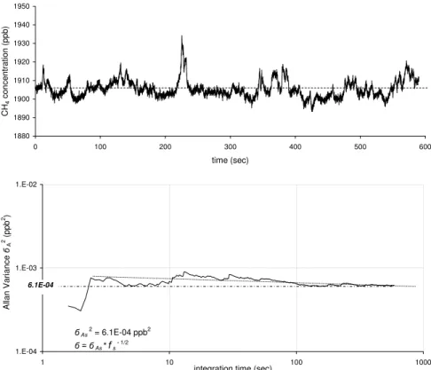
over a ten minute period of relative constant CH₄concentrations (Fig. 3) with a mean value of 1905 ppb and a standard deviation of 4.74 ppb with 10 Hz sampling rate were used to determine the Allan variance. Subsequently, the Allan variance of this period was plotted over the integration time T (Fig. 3), showing a decreasing Allan variance over integration times larger than 2.4 s. No increase of the Allan variance was ob-15

served at larger integration times, indicating an absence of instrumental drift, and thus high system stability and sensitivity, for integration times of a few seconds up to ten minutes. Additionally, an indication for the short term precision (σ) could be obtained by the y-axis interception point at the minimum Allan variance (σ_As2 =6.1×10−3ppb2). Using Eq. (4):

20

σ=σ_As×f_s−1/2 (4)

in whichσAs is the square root of the minimum Allan variance andfs is the sampling

frequency of the system (10 Hz),σwas determined as 7.81×10−3ppb.

As long as ambient temperatures do not exceed the range of 5 to 45◦C, the DLT-100 the temperature (T_cell) will stay in a range tolerable for good performance. The pressure 25

(9)

ACPD

7, 11587–11619, 2007

Title Page

Tables Figures

◭ ◮

Back Close

Full Screen / Esc

EGU

in the measurement (Pcell) is mainly dependent on pump capacity, the amount and type

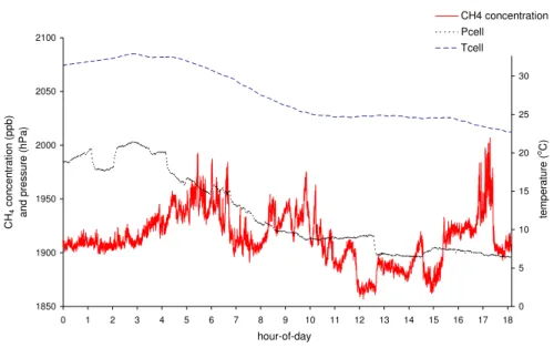
of filtering and tubing, but should be kept in the range of 190 to 210 hPa. Within these boundary conditions the influence of changing temperature and pressure conditions in the measurement cel on CH4concentration measurements were assessed (Fig. 4). It

can be observed that relatively large changes of T_cell as well as P_cell do not have an 5

influence on the CH4 concentration measurements. However, Tcell and Pcell do show

a linear relation, in accordance with the ideal gas law.

A calibration experiment was carried out by administering standard gas mixtures with concentrations of 125 ppb and 2002 ppb CH4respectively, both with a precision of

0.2 ppb, to the FMA at ten moments within a 10-day period. During the whole experi-10

ment the FMA was never turned of in order to imitate longer measurement periods as will be the case in the field set-up. Although the measured concentration sometimes varied one or two ppb over the experimental period for both gases, no actual drift was observed in the analyser (Table 1). Calibration factors are 1 on average and fluctuate only very slightly.

15

Additionally, over a period of a week, CH4concentration measurements at the 4.3 m

high tower at the Horstermeer site were compared with CH₄concentrations measured at 20 and 60 m height at a measurement site in Cabauw (51◦58′N and 4◦55′E), ap-proximately 30×103m from the Horstermeer site1. The CH4concentrations at Cabauw

were measured with a Carlo Erba gas Chromatograph system and have a precision of 20

2 ppb. The CH4concentration at the Horstermeer site was 15 ppb higher on average,

which might be the result of the relatively high CH4 emissions from the peat meadow

area in which the measurements were taken. None the less, the increasing trend of CH4 concentration at the Horstermeer site was similar to the trend at the Cabauw

site. Generally, slow variation in concentrations is caused by the difference between 25

continental and marine background concentration, the continental concentration being approximately 50 ppb higher (Eisma et al., 1994). During the measurement period,

1

The CH₄concentration measurements in Cabauw are measured with a gas chromatograph

(10)

ACPD

7, 11587–11619, 2007

Title Page

Tables Figures

◭ ◮

Back Close

Full Screen / Esc

EGU

winds from eastern, continental, direction prevailed, which accounted for the slow rise in CH₄concentrations at the measurement locations.

In general a sampling rate of 10 Hz, with a Nyquist frequency of 5 Hz, is used for eddy covariance techniques (Aubinet et al., 2000; Kroon et al., 2007). The measure-ment rate of an instrumeasure-ment is determined by both electronic signal processing and by 5

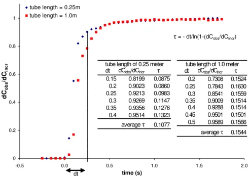
the signal response time of the measurement cell (τ) (Nelson et al., 2004). Electronic signal processing is dependent on the spectral complexity of the measurement tech-nique as well as the technical design of the ICOS techtech-nique. In the case of the FMA, this was defined by the designers (LGR Ltd.) as 20 Hz. The limiting factor of the max-imum sampling rate is oftenτ, which could be determined as the 63% (1–1/e) of the 10

instrument response after applying a step change in concentration at 20 Hz sampling rate (Moore, 1986; Zahniser et al, 1995). In this, sensitivity to tube length (Fig. 5) could be observed. Since the effect of tube damping is corrected separately, andτonly refers to the response of the instrument itself, the actualτ is determined as 0.10 s, which is in close agreement with the value expected from the volume of outside air in the mea-15

surement cell (0.11×10−3m3) divided by the pumping speed (1.0×10−3m3s−1). Theτ

includes an underestimation of 37% (1/e) of the signal, which was corrected for during the data processing.

The time lag of the CH4 measurements in the field set-up at a 10 Hz sampling rate

was estimated at 0.6 s by determining the maximum covariance ofw′and the deviation 20

of the CH4concentration[CH4]

′

forw′at t=0.0 s and[CH4]

′

at t=0.1 s, t=0.2 s, t=0.3 s, etc.

3.2 Data treatment

Data were logged digitally on a handheld computer at a rate of 10 Hz (Van der Molen et al., 2006). The EUROFLUX methodology (Aubinet et al., 2000) was applied to the 25

eddy covariance data to calculate the CO2fluxes from the open path system (Hendriks

et al., 2007) and the CH₄ fluxes from the closed path system on a thirty minute basis. Since system instrumental drift was not observed, an overestimation of the fluxes as a

(11)

ACPD

7, 11587–11619, 2007

Title Page

Tables Figures

◭ ◮

Back Close

Full Screen / Esc

EGU

result of this averaging period was not expected. The effect of the measurement cell response timeτ on the CH₄ signal was corrected for in the flux calculation procedure as well as for the time lag of 0.6 s between closed path CH4 and open path wind, tem-perature and CO2measurements. The tube length of the set-up was over 1000 times

the length of the diameter of the tube and therefore the air temperature in the mea-5

surement cell can be considered stable. Therefore the Webb correction for density fluctuations arising from variations in temperature that was applied to the open path CO₂measurements is not required for the closed path measurements of CH₄(Leuning and Moncrieff, 1990). The Webb correction for density fluctuations arising from varia-tions in water vapour (measured with the Licor 7500) was applied according to Leuning 10

and Moncrie_ff (1990). Frequency loss corrections for closed-path systems were ap-plied according to the theory of Leuning and King (1992). The method of Nakai et al. (2006) was used to apply the angle of attack dependent calibration (Gash and Dolman, 2003; Van der Molen et al., 2004).

3.3 Validity of the measurement set-up and data 15

Spectral and co-spectral analysis of the fluctuations ofw, air temperature (T) and CH4

concentration [CH4] in the atmosphere associated with turbulent transport are

per-formed to assess the reliability of flux measurements (Stull et al., 1988; Kaimal and Finnigan, 1994). We determined spectra of thew,T and [CH4] as well as co-spectra of

temperature fluxes (w′T′) and CH4fluxes (w’[CH4]′) using raw 10 Hz eddy covariance

20

data of four 30 min periods in summer (Fig. 6). The power spectra and co-spectra are binned and plotted as a function of frequency on a log-log scale. Spectra forw,T and [CH4] as well as the co-spectra w′T′ and w’[CH4]′ have corresponding slopes

show-ing a proportionality of −2/₃, which is in agreement with the power law in the inertial sub-range (Eugster and Senn, 1994). This indicated that the eddy covariance set-up 25

records nearly all fluctuations of [CH4] associated with turbulent transport (Goulden

(12)

ACPD

7, 11587–11619, 2007

Title Page

Tables Figures

◭ ◮

Back Close

Full Screen / Esc

EGU

discussed in a previous paper by Hendriks et al. (2007). The shapes of the power- and co-variance spectra for [CH₄] were comparable to the [CO₂] spectra and the energy balance showed a closure of 82%. This implied that the data from the eddy covariance set-up are acceptable (Lloyd et al., 1996).

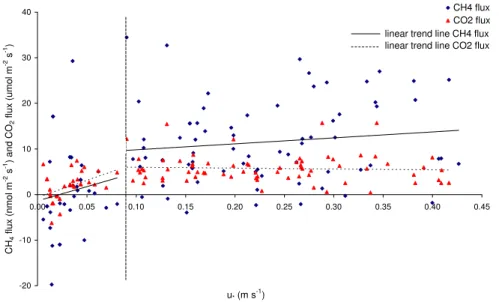
During night time periods with low friction velocity (u_∗) the turbulence of the air can be 5

too low for the performance of eddy covariance measurements. In order to determine the critical u_∗ values at this specific site (Wohlfahrt et al., 2005), the flux data for CH4

and CO₂of night time periods were plotted versus u_∗(Fig. 7). The nightly CH₄ fluxes indeed decreased for u_∗<0.09 m s−1similar to the decrease in CO2flux.

4 CH₄ eddy covariance data-series and comparison with flux chamber

mea-10

surements and high tower data

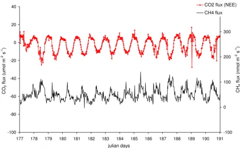
The CH4 fluxes and CO2 fluxes (net ecosystem exchange (NEE)) were plotted for a

two week period in June 2006 at the Horstermeer site (Fig. 8). Both data series were corrected for low u_∗values and gaps were filled with data of the surrounding half hours when small (max. two half hourly periods) or by data of the same point in time of the 15

preceding day (max. ten half hourly periods). Although the CH4 emissions are rather

variable over time, a diurnal pattern can be observed with lower fluxes during the night and high fluxes during the day. CO2fluxes have a similar, but opposite, diurnal cycle.

The average CH4emission was 50±12.5 nmol m− 2

s−1, while the typical maximum CH4

emission was 120±30 nmol m−2s−1(during daytime) and the typical minimum flux was 20

–20±2.5 nmol m−2s−1(uptake, during night time). Uncertainties of the CH₄ emissions were estimated at 25% of the half hourly flux data, based on uncertainty estimates of CO2eddy covariance data resulting from errors in measurement set-up, data

process-ing and gap fillprocess-ing (Hendriks et al., 2007).

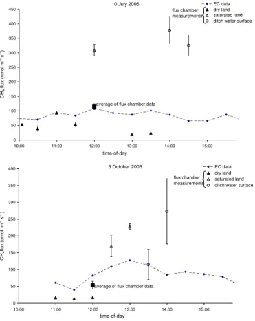
For two days during the CH4 eddy covariance measurement period at the

Horster-25

meer peat meadow site, flux chamber measurements were made in the footprint of the eddy covariance tower with a Photo Acoustic Field Gas-Monitor (type 1312,

(13)

ACPD

7, 11587–11619, 2007

Title Page

Tables Figures

◭ ◮

Back Close

Full Screen / Esc

EGU

nova AirTech Instruments, Ballerup, Denmark) connected with tubes to closed, dark chambers (Hendriks et al., 2007). Flux chamber data were collected at the three land elements occurring in the footprint of the eddy covariance tower: relatively dry peat land, saturated peat land and ditch water surfaces. The fluxes from the various land elements are averaged with respect to their relative surface area (70%, 20% and 10% 5

respectively; Hendriks et al., 2007)). At the 10 June the flux chamber measurements showed an average CH4flux of 114±10 nmol m−

2

s−1, while the eddy covariance mea-surements showed an average CH₄flux of 83±21 nmol m−2s−1 over the same period (Fig. 9). On the 3 of October the average CH4 flux from the chamber measurements

was 54±11 nmol m−2s−1, while that of the eddy covariance was 61±15 nmol m−2s−1. 10

5 Alternative eddy covariance measurement types

In eddy covariance, the sampling rate determines the number of samples that are taken out of an infinitely large number of samples. The higher the sampling rate, the higher the statistical reliability, which results in higher accuracy of the observed means and covariances (Van der Molen, 2002). In order to obtain reliable estimates of fluxes, 15

a sampling rate of at least 10 Hz is generally used for eddy covariance techniques. However, measurements performed at lower rates than 10 Hz generate results of cer-tain reliability too. Disjunct eddy covariance, slow 1 Hz eddy covariance and REA are possible alternatives for the preferred 10 Hz eddy covariance. These measurement techniques could make the external pump of the FMA eddy covariance set-up super-20

fluous and thus save over half of the energy required for the eddy covariance set-up. This might be inevitable to operate the set-up it in remote places where 220 V is not available.

(14)

ACPD

7, 11587–11619, 2007

Title Page

Tables Figures

◭ ◮

Back Close

Full Screen / Esc

EGU

determine the flux of an atmospheric propertyF_s according to Eq. (5):

Fs=< w′s′>=

1

N×

N

X

i=1

w_i′s_i′ (5)

whereN is the subset of the data (Rinne et al., 2000 and 2001). Here, the disjunct eddy covariance method was tested by sampling the first data point of every 10 data points from the 10 Hz data set, thereby creating a time interval of 0.9 s between the 5

sampling moments, while the measurement cell response time remained 0.10 s. To build a field set-up for disjunct 1 Hz eddy covariance a “snap sampling” instrument would have to be mounted in front of the inlet of the system to obtain samples that are sampled with a frequency of 1 Hz, while maintaining the sampling duration as short as possible (“snap”). This method would give the FMA an analysis time of 1.0 s instead of 10

0.10 s.

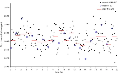
With slow 1 Hz eddy covariance, F_s is determined in the same manner as 10 Hz eddy covariance (Eq. 2), but withdt=1.0 s instead of 0.10 s. The method was tested by averaging each 10 consecutive data points of CH₄ concentration as well as wind velocity for all variables of the 10 Hz data set (Fig. 10), thereby simulating a slower 15

sampling rate (1 Hz) with a longer response time (1.0 s instead of 0.10 s).

REA is a conditional sampling method in which air samples are drawn to two sepa-rate reservoirs depending on the direction ofw. The criterion of valve switching was based on values of the standard deviation ofw (σ_w), which is measured by a sonic anemometer at 10 Hz. The valve is activated according to the threshold condition 20

|w0|=0.6σw. In the case of −w0≤w≤w0 (deadband values), neither “up” nor “down”

samples were taken, but samples are discarded from the sampling system (Graus et al., 2006). Here, we simulated REA by dividing all eddy covariance data points of one half hour measurement period into three data matrixes based on the direction of the

w(upward, downward and deadband values). Next, the measured concentrations are 25

summed and the turbulent flux of the scalars(Fs) was determined according to Eq. (6):

Fs≈b×σw×∆s (6)

(15)

ACPD

7, 11587–11619, 2007

Title Page

Tables Figures

◭ ◮

Back Close

Full Screen / Esc

EGU

(Businger and Oncley, 1990), whereb is the correction for the deadband and∆s the difference between the concentrations in the accumulation reservoirs (Bowling et al., 1999). Pattey et al. (1993) determined the value ofbto be 0.56, but after testing for the measurement set-up investigated here, ab-value of 0.70 showed results most similar to the normal 10 Hz eddy covariance measurements.

5

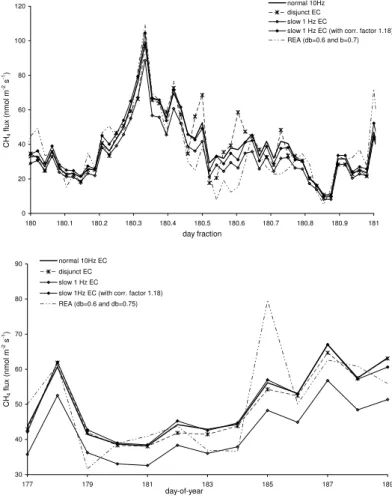
Data were compared with normal 10 Hz eddy covariance data as half hourly data series and as daily averages over a two-week period (Table 2 and Fig. 11). The dis-junct eddy covariance method resulted in CH4emissions that were in fact very similar

10 Hz eddy correlation data, but showed small random deviations at a half hourly ba-sis. On daily basis the disjunct eddy covariance showed a maximum underestimation of 10

–5.4%, while on average the underestimation was only –1.4%. The slow 1 Hz eddy co-variance method rather constantly underestimated the normal 10 Hz eddy coco-variance by –15.5% on average, both on the half hourly and the daily basis. This underestima-tion was the e_ffect of averaging turbulent perturbations, enabling the set-up to measure CH4 molecules transported by high frequent atmospheric turbulence (>1 Hz).

How-15

ever, in the Horstermeer polder no daily patterns were found in the underestimation of the emission, which could be explained by the characteristics of the measurement location: a flat, open and windy grass land site with a well mixed atmosphere. A single correction factor of 1.18 could be applied to the slow 1 Hz eddy covariance data, af-ter which the normal 10 Hz eddy covariance data were very well matched by the slow 20

1 Hz eddy covariance data. The REA method resulted in half hourly data that showed considerable random deviations from the normal 10 Hz eddy correlation data, having a standard deviation twice as large as that of the normal eddy covariance (Table 2). Additionally, on a daily basis the trends observed by the normal 10 Hz eddy covariance were not matched very well. However, the average deviation from the normal 10 Hz 25

(16)

ACPD

7, 11587–11619, 2007

Title Page

Tables Figures

◭ ◮

Back Close

Full Screen / Esc

EGU

6 Conclusions

The new fast methane analyser, which uses the new off-axis integrated cavity out-put spectroscopy technique, was found to perform satisfactory in field and lab tests. Compared to other techniques the absence of a large nitrogen Dewar for cooling that would need weekly refill, the compact, narrow band and stable laser, the relatively 5

user friendliness and low costs are considerable advantages. However, care should be taken when placing the instrument with a scroll pump in the field. The instrument should be kept dry and in ambient temperatures between 5◦C and 45◦C, while the scroll pump should be kept dry and cool. Contamination of the measurement cell should be prevented, since the mirrors inside the measurement cell are sensitive and only 10

a small contamination might cause a rapid decrease in reflectivity of the mirrors and performance of the instrument. Cleaning of the mirrors, however, is a relatively simple procedure that can be done by the user himself in a dust-free environment.

The analysis of the Allan Variance indicated a high precision and system stability of the FMA. Additionally, since instrumental drift was observed neither in the calibration 15

experiment nor in the comparison with high tower data, it was concluded that frequent calibration of the FMA is indeed not necessary. The measurement cell response time was tested to be 0.10 s with a 37% underestimation of the measured signal, which was corrected for during the data processing. As long as ambient temperatures do not exceed the range of 5 to 45◦C and pressure in the measurement cell is near 205 hPa, 20

the CH4 measurements are not affected by changes in temperature and pressure in

the measurement cell. Concluding, the instrument appeared very well suitable for eddy covariance measurements.

The FMA eddy covariance system performed well, as shown by the power- and co-spectra as well as by the closure of the energy balance. CH₄and CO₂fluxes appeared 25

to respond similar to low u_∗ values and therefore a u_∗ correction was applied for CH4

fluxes in the same manner as for CO2fluxes. CH4 emissions are rather variable over

(17)

ACPD

7, 11587–11619, 2007

Title Page

Tables Figures

◭ ◮

Back Close

Full Screen / Esc

EGU

while the typical maximum CH4emission is 120±30 nmol m− 2

s−1(during daytime) and the typical minimum flux is 20±2.5 nmol m−2s−1(uptake, during night time). These CH4

fluxes are in agreement with the QCL flux measurements at managed peat meadow site in the Netherlands (Reeuwijk), where emissions are 40±31 nmol m−2s−1 on aver-age (Kroon et al., 2007) and averaver-age annual CH4 emission of 30 nmol m−

2

s−1 from 5

peat lands in Germany and the Netherlands (Dr ¨osler et al., 2007). From the com-parison of the eddy covariance measurements with flux chamber measurements was observed that the fluxes from the two techniques lie in the same order of magnitude. However, considering the fact that the flux chamber measurements are point mea-surements at the soil surface while the eddy covariance has a footprint of hundreds of 10

square meters, some degree of variation may be expected.

Additionally, the set-up was tested for three measurement techniques with slower measurement rates, which could be used in the future to make the scroll pump su-perfluous and save energy. Both disjunct eddy covariance as well as slow 1 Hz eddy covariance showed results very similar to 10 Hz eddy covariance. Relaxed eddy ac-15

cumulation performed less well on half hourly and daily basis. However, over periods of at least several weeks, net emission showed only a slight deviation from the normal 10 Hz eddy covariance data. It was concluded that, when using a scroll pump is not possible for technical or practical reasons; both disjunct eddy covariance and slow 1 Hz eddy covariance are reliable substitutes for normal 10 Hz eddy covariance.

20

Acknowledgements. This research project is performed in the framework of the European re-search programme Carbo Europe (contract number GOCE-CT2003-505572) and the Dutch

National Research Programme Climate Changes Spatial Planning (www.klimaatvooruimte.nl).

Also, we would like to thank our technical co-operators R. Stoevelaar and R. Lootens.

References

25

(18)

ACPD

7, 11587–11619, 2007

Title Page

Tables Figures

◭ ◮

Back Close

Full Screen / Esc

EGU Aubinet, M., Grelle A., Ibrom, A., et al.: Estimates of the annual net carbon and water exchange

of forests: The EUROFLUX methodology, Adv. Ecol. Res., 30, 30, 113–175, 2000.

Bear, D. S., Paul, J. B., Gupta, M., et al.: Sensitive absorption measurements in the near-infrared region using off-axis integrated-cavity-output spectroscopy, Appl. Phys. B, 75, 261– 265, 2002.

5

Bowling, D. R., Delany, A. C., Turnipseed, A. A., et al.: Modification of the relaxed eddy ac-cumulation technique to maximize measured scalar mixing ratio differences in updrafts and downdrafts, J. Geophys. Res.-Atmos., 104(D8), 9121–9133, 1999.

Businger, J. A. and Oncley, S. P.: Flux Measurement with Conditional Sampling, J. Atmos. Ocean. Tech., 7(2), 349–352, 1990.

10

Dr ¨osler, M., Freibauer, A., Christensen, T. R., et al.: Observations and status of peatland greenhouse gas emissions in Europe. In: Dolman, A. J., Valentini, R. and Freibauer, A.: Observing the continental scale greenhouse gas balance, Chapter 8, to be published in Springer Ecological series, 2007.

Eisma, R., Vermeulen, A. T., and Kieskamp, W. M.: Determination of European methane emis-15

sions, using concentration and isotope measurements, Environ. Monit. Assess., 31, 197– 202, 1994.

Faist, J., Capasso, F., Sivco, D. L., et al.: Quantum Cascade Laser – Temperature-Dependence of the Performance-Characteristics and High T0 Operation, Appl. Phys. Lett., 65(23), 2901– 2903, 1994.

20

Gash, J. H. C. and Dolman, A. J.: Sonic anemometer (co)sine response and flux measurement I. The potential for (co)sine error to affect sonic anemometer-based flux measurements, Agr. Forest Meteorol., 119(3–4), 195–207, 2003.

Goulden, M. L., Munger, J. W., Fan, S. M. et al.: Measurements of carbon sequestration by long-term eddy covariance: Methods and a critical evaluation of accuracy. Glob. Change 25

Biol., 2(3), 169–182, 1996.

Graus, M., Hansel, A. Wisthaler, A., et al.: A relaxed-eddy-accumulation method for the mea-surement of isoprenoid canopy-fluxes using an online gas-chromatographic technique and PTR-MS simultaneously, Atmos. Environ., 40, S43–S54, 2006.

Hargreaves, K. J., Fowler, D., et al.: Annual methane emission from Finnish mires estimated 30

from eddy covariance campaign measurements, Theor. Appl. Climatol., 70(1-4), 203–213, 2001.

Hendriks, D. M. D., van Huissteden, J., Dolman, A. J., van der Molen, M. K.: The full greenhouse

(19)

ACPD

7, 11587–11619, 2007

Title Page

Tables Figures

◭ ◮

Back Close

Full Screen / Esc

EGU gas balance of an abandoned peat meadow, Biogeosciences, 4, 411–424, 2007,

http://www.biogeosciences.net/4/411/2007/.

IPCC: IPCC Fourth Assessment Report, Climate Change 2007, Cambridge Univ. press., Cam-bridge, UK, 2007.

Kaimal, J. C. and Finnigan, J. J.: Atmospheric boundary layer flows, their structure and man-5

agement, New York, Oxford University Press, 33–65, 208–280, 1994.

Kormann R., Muller, H., Werle, P.: Eddy flux measurements of methane over the fen “Murnauer Moos”, 11 degrees 11 ’ E, 47 degrees 39 ’ N, using a fast tunable diode laser spectrometer, Atmos. Environ., 35(14), 2533–2544, 2001.

Kroon, P. S., Hensen, A., Zahniser, M. S., et al.: Suitability of quantum cascade laser spec-10

trometry for CH₄ and N₂O eddy covariance measurements, Biogeosciences Discuss., 2,

1137–1165, 2007,

http://www.biogeosciences-discuss.net/2/1137/2007/.

Leuning, R. and Moncrieff, J. : Eddy-Covariance CO₂ Flux Measurements Using Open-Path

and Closed-Path Co2 Analyzers – Corrections for Analyzer Water-Vapour Sensitivity and 15

Damping of Fluctuations in Air Sampling Tubes, Bound.-Lay. Meteorol., 53(1–2), 63–76, 1990.

Leuning, R. and King, K. M.: Comparison of eddy-covariance measurements of CO₂fluxes by

open-path and closed path CO₂analysers. Bound.-Lay. Meteorol., 59 (3), 297–311, 1992.

Nakai, T., van der Molen, M. K., Gash, J. H. C., et al.: Correction of sonic anemometer angle of 20

attack errors, Agr. Forest. Meteorol., 136(1-2), 19–30, 2006.

Nelson, D. D., McManus, B., Urbanski, S., et al.: High precision measurements of atmospheric nitrous oxide and methane using thermoelectrically cooled mid-infrared quantum cascade lasers and detectors, Spectrochim. Acta. A, 60(14), 3325–3335, 2004.

O’Keefe, A.: Integrated cavity output analysis of ultra-weak absorption, Chem. Phys. Lett., 25

293(5–6), 331–336, 1998.

Pattey, E., Desjardins, R. L., and Rochette, P.: Accuracy of the Relaxed Eddy-Accumulation

Technique, Evaluated Using CO₂ Flux Measurements, Bound.-Lay. Meteorol., 66(4), 341–

355, 1993.

Rinne, H. J. I., Delany, A. C., Greenberg, J. P., et al.: A true eddy accumulation system for 30

trace gas fluxes using disjunct eddy sampling method, J. Geophys. Res.-Atmos., 105(D20), 24 791–24 798, 2000.

(20)

ACPD

7, 11587–11619, 2007

Title Page

Tables Figures

◭ ◮

Back Close

Full Screen / Esc

EGU trace gas flux measurements, Geophys. Res. Lett., 28(16), 3139–3142, 2001.

Stull, R. B.: An Introduction to boundary layer meteorology, Dordrecht, Kluwer Academic Pub-lishers, Atmospheric Sciences Library, Chapter 8, 1988.

Van der Molen, M. K.: Meteorological impacts of land use change in the Maritime tropics, Chapter 3, Data analysis, Thesis, Vrije Universiteit, 35–72, 2002.

5

Van der Molen, M. K., Gash, J. H. C., Elbers, J. A., et al.: Sonic anemometer (co)sine response and flux measurement – II. The effect of introducing an angle of attack dependent calibration, Agr. Forest Meteorol., 122(1-2), 95–109, 2004.

Van der Molen, M. K., Zeeman, M. J., Lebis, J., et al.: EClog: A handheld eddy covariance logging system, Comput. Electron. Agr., 51(1–2), 110–114, 2006.

10

Werle, P., Mucke, R., and Slemr, F.: The Limits of Signal Averaging in Atmospheric Trace-Gas Monitoring by Tunable Diode-Laser Absorption-Spectroscopy (Tdlas), Appl. Phys. B-Photo, 57(2), 131–139, 1993.

Wohlfahrt, G., Anfang, C., Bahn, M., et al.: Quantifying nighttime ecosystem respiration of a meadow using eddy covariance, chambers and modelling, Agr. Forest Meteorol., 128(3–4), 15

141–162, 2005.

Zahniser, M. S., Nelson, D. D., McManus, J. B., et al.: Measurement of Trace Gas Fluxes Using Tunable Diode-Laser Spectroscopy. Philosophical Transactions of the Royal Society of London, Series a-Mathematical Physical and Engineering Sciences, 351(1696), 371–381, 1995.

20

(21)

ACPD

7, 11587–11619, 2007

Title Page

Tables Figures

◭ ◮

Back Close

Full Screen / Esc

EGU

Table 1. Results of the 10-day calibration experiment with two standard gases of 125 and

2002 ppb respectively. Time elapsed since start of experiment; CH₄concentrations measured

by FMA, deviation from the actual concentration and calibrations factor are shown.

concentrations measured with FMA

measurement time elapsed low CH4gas (125 ppb) high CH4gas (2002 ppb) calibration

(date and time) (days) (ppb) (deviation) (ppb) (deviation) factor

(22)

ACPD

7, 11587–11619, 2007

Title Page

Tables Figures

◭ ◮

Back Close

Full Screen / Esc

EGU

Table 2.Summary of results of disjunct eddy covariance, slow 1 Hz eddy covariance (with and

without correction factor) and REA compared to normal 10 Hz eddy covariance. Half hourly data, average emissions, standard deviations and deviation from the normal 10 Hz eddy co-variance are shown for all measurement techniques.

two week average half hourly data daily averages emission

(nmol m−2s−1)

deviation from 10 Hz data

stand. dev. (nmol m−2s−1)

max. de-viation

stand. dev. (nmol m−2s−1)

max. de-viation

normal 10 Hz EC 50.90 0.0% 23.46 0% 9.53 0.0%

disjunct 1 Hz EC 49.40 –1.4% 24.60 60% 9.50 –5.4%

slow 1 Hz EC 42.48 –15.2% 20.44 50% 7.89 –18.8%

slow 1 Hz EC (corrected with factor 1.18)

50.13 0.1% 24.12 35% 9.31 –4.2%

REA (d=0.6 and b=0.75) 49.93 –0.3% 47.92 >100% 13.15 41.9%

(23)

ACPD

7, 11587–11619, 2007

Title Page

Tables Figures

◭ ◮

Back Close

Full Screen / Esc

EGU

Fig. 1. Schematic overview of the off-axis integrated cavity output spectrometry (ICOS)

(24)

ACPD

7, 11587–11619, 2007

Title Page

Tables Figures

◭ ◮

Back Close

Full Screen / Esc

EGU

data from Gill to handheld system

data from Gill to handheld system 1+2

3

4

7

5

8 8

10 11

12

15

direction data flow

direction air flow

3x25A; 220V 17 14

6

9 16

13

1 rain cap (sharpened at the edges) 2 filter (60 um?)

3 bended tubing of rust free steel 4 teflon tubing (diameter=64 mm) 5 water locked case 6 tube with warming strip 7 Fast Methane Analyser 8 heating elements

9 sturdy pipe to pump (large diameter) 10 semi closed case

11 scroll pomp 12 air exhaust with silencer 13 Gill sonic anemometer

14 Licor7500 (CO2, T and H2O analyser)

15 data collection in Gill software 16 handheld computer

17 power supply (regional electricity network) swagelock screws are used for all connections

Fig. 2. Schematic overview of the combined field set-up of the open path eddy covariance

system for carbon dioxide and water vapour and the closed path eddy covariance system for methane using the FMA.

(25)

ACPD

7, 11587–11619, 2007

Title Page

Tables Figures

◭ ◮

Back Close

Full Screen / Esc

EGU

1880 1890 1900 1910 1920 1930 1940 1950

0 100 200 300 400 500 600

time (sec)

CH

4

co

ncen

tra

ti

o

n (

ppb

)

1.E-04 1.E-03 1.E-02

1 10 100 1000

integration time (sec)

Al

la

n

Va

ri

a

n

ce

бA 2 (p

pb

2)

бAs

2

= 6.1E-04 ppb2

б = бAs*fs

-1/2

6.1E-04

Fig. 3. Time series of CH₄concentration measurements with 10 Hz sampling rate with a mean

(26)

ACPD

7, 11587–11619, 2007

Title Page

Tables Figures

◭ ◮

Back Close

Full Screen / Esc

EGU

1850 1900 1950 2000 2050 2100

0 1 2 3 4 5 6 7 8 9 10 11 12 13 14 15 16 17 18

hour-of-day

CH

4

concen

tration

(pp

b

)

and p

ressur

e

(

h

P

a

)

0 5 10 15 20 25 30 35

tem

per

atur

e (

oC)

CH4 concentration Pcell

Tcell

Fig. 4. FMA data from a measurement day in spring. P_cell ranges from 190 to 201 hPa and

T_cell ranges from 22.7 to 32.9◦C. Fluctuations in CH₄ concentration measurements show no

dependence on P_cellor T_cell.

(27)

ACPD

7, 11587–11619, 2007

Title Page

Tables Figures

◭ ◮

Back Close

Full Screen / Esc

EGU

0 0.2 0.4 0.6 0.8 1

-0.5 0.0 0.5 1.0 1.5 2.0

time (s)

dC

ob

s

/d

Cin

c

r

tube length = 0.25m tube length = 1.0m

dt

τ = - dt/ln(1-(dCobs/dCincr)

dt dCobs/dCincr τ

0.2 0.7308 0.1524 0.25 0.7843 0.1630 0.3 0.8541 0.1559 0.35 0.9009 0.1514 0.4 0.9288 0.1514 0.45 0.9501 0.1501 0.5 0.9589 0.1566

averageτ 0.1544 tube length of 1.0 meter dt dCobs/dCincr τ

0.15 0.8199 0.0875 0.2 0.9023 0.0860 0.25 0.9213 0.0983 0.3 0.9269 0.1147 0.35 0.9356 0.1276 0.4 0.9514 0.1323 averageτ 0.1077 tube length of 0.25 meter

Fig. 5. Normalized and averaged time series showing 63% instrument response with 20 Hz

(28)

ACPD

7, 11587–11619, 2007

Title Page

Tables Figures

◭ ◮

Back Close

Full Screen / Esc

EGU

-2/3 -2/3

Fig. 6.Results from spectral analyses ofw,T and [CH₄] and (co-)spectral analyses ofw′T′and

w’[CH₄]′, showing the required slopes of –2/₃ under turbulent circumstances. Analyses were done over four half hours of 10 Hz data which were separately binned.

(29)

ACPD

7, 11587–11619, 2007

Title Page

Tables Figures

◭ ◮

Back Close

Full Screen / Esc

EGU

-20 -10 0 10 20 30 40

0.00 0.05 0.10 0.15 0.20 0.25 0.30 0.35 0.40 0.45

u* (m s -1

)

CH

4

f

lux

(nmol

m

-2 s -1) a

nd

CO

2

fl

ux (umol

m

-2 s -1)

CH4 flux CO2 flux linear trend line CH4 flux linear trend line CO2 flux

Fig. 7. Results of the analyses of the effect of variation in u_∗ on nightly CH₄ and CO₂ fluxes,

(30)

ACPD

7, 11587–11619, 2007

Title Page

Tables Figures

◭ ◮

Back Close

Full Screen / Esc

EGU

-100 -80 -60 -40 -20 0 20 40

177 178 179 180 181 182 183 184 185 186 187 188 189 190 191

julian days

CO

2

f

lux

(umol

m

-2 s -1)

-100 0 100 200 300 400

CH

4

f

lux

(n

mol

m

-2 s -1)

CO2 flux (NEE)

CH4 flux

Fig. 8.Graph of CH₄flux data series over a two week period in the summer of 2006, combined

with CO₂flux (NEE) data series over the same period.

(31)

ACPD

7, 11587–11619, 2007

Title Page Abstract Introduction Conclusions References Tables Figures ◭ ◮ ◭ ◮ Back Close

Full Screen / Esc

Printer-friendly Version Interactive Discussion EGU 0 50 100 150 200 250 300 350 400 450

10:00 11:00 12:00 13:00 14:00 15:00

time-of-day CH 4 f lux (nmol m

-2 s -1)

EC data dry land saturated land ditch water surface

average of flux chamber data

10 July 2006

flux chamber measurements 0 50 100 150 200 250 300 350 400

10:00 11:00 12:00 13:00 14:00 15:00

time-of-day CH 4 fl ux (umol m

-2 s -1)

EC data dry land saturated land ditch water surface

average of flux chamber data

3 October 2006

flux chamber measurements

Fig. 9. Hourly CH₄flux data at 10 July and 3 October the (both 2006) plotted in combination

(32)

ACPD

7, 11587–11619, 2007

Title Page

Tables Figures

◭ ◮

Back Close

Full Screen / Esc

EGU

2400 2420 2440 2460 2480 2500 2520 2540

0 1 2 3 4 5 6 7 8 9 10 11 12 13 14 15 16 17 18 19 20

time (s)

CH

4

c

onc

ent

rat

ion

(ppb)

normal 10Hz EC disjunct EC slow 1Hz EC

Fig. 10. Example of data sampling for the various measurement types: measured

concentra-tions for normal 10 Hz eddy covariances, disjunct eddy covariance and slow 1 Hz eddy covari-ance. Disjunct eddy covariance takes every first sample point of a 10 Hz data series and slow eddy covariance takes the average of ten sample points of a 10 Hz data series.

(33)