www.biogeosciences.net/12/3925/2015/ doi:10.5194/bg-12-3925-2015
© Author(s) 2015. CC Attribution 3.0 License.
Eddy covariance methane flux measurements over a grazed pasture:
effect of cows as moving point sources
R. Felber1,2, A. Münger3, A. Neftel1, and C. Ammann1
1Agroscope Research Station, Climate and Air Pollution, Zurich, Switzerland 2ETH Zurich, Institute of Agricultural Sciences, Zurich, Switzerland
3Agroscope Research Station, Milk and Meat Production, Posieux, Switzerland
Correspondence to:R. Felber ([email protected])
Received: 21 January 2015 – Published in Biogeosciences Discuss.: 24 February 2015 Revised: 26 May 2015 – Accepted: 08 June 2015 – Published: 29 June 2015
Abstract. Methane (CH4) from ruminants contributes
one-third of global agricultural greenhouse gas emissions. Eddy covariance (EC) technique has been extensively used at var-ious flux sites to investigate carbon dioxide exchange of ecosystems. Since the development of fast CH4 analyzers,
the instrumentation at many flux sites has been amended for these gases. However, the application of EC over pastures is challenging due to the spatially and temporally uneven dis-tribution of CH4 point sources induced by the grazing
ani-mals. We applied EC measurements during one grazing sea-son over a pasture with 20 dairy cows (mean milk yield: 22.7 kg d−1) managed in a rotational grazing system.
Individ-ual cow positions were recorded by GPS trackers to attribute fluxes to animal emissions using a footprint model. Methane fluxes with cows in the footprint were up to 2 orders of mag-nitude higher than ecosystem fluxes without cows. Mean cow emissions of 423±24 g CH4head−1d−1(best estimate from
this study) correspond well to animal respiration chamber measurements reported in the literature. However, a system-atic effect of the distance between source and EC tower on cow emissions was found, which is attributed to the analyti-cal footprint model used. We show that the EC method allows one to determine CH4emissions of cows on a pasture if the
data evaluation is adjusted for this purpose and if some cow distribution information is available.
1 Introduction
Methane (CH4) is, after carbon dioxide (CO2), the second
most important human-induced greenhouse gas (GHG), con-tributing about 17 % of global anthropogenic radiative forc-ing (Myhre et al., 2013). Agriculture is estimated to con-tribute about 50 % of total anthropogenic emissions of CH4,
while enteric fermentation of livestock alone accounts for about one-third (Smith et al., 2007). For Switzerland these numbers are even higher, with 85 %total agricultural contri-bution and 67 % from enteric fermentation alone, although still afflicted with considerable uncertainty (Hiller et al., 2014). Measurements of these emissions are therefore im-portant for national GHG inventories and for assessing their effect on the global scale.
Direct measurements of enteric CH4emissions are
com-monly made on individual animals using open-circuit respi-ration chambers (Münger and Kreuzer, 2006, 2008) or the SF6 tracer technique (Lassey, 2007; Pinares-Patiño et al.,
2007). Both methods are labor intensive and thus are usu-ally applied only for rather short time intervals (several days). Although the respiration chamber method requires costly in-frastructure and investigates animals in spatially constraint conditions, it presently is the reference technique for esti-mating differences in CH4emissions related to animal breed
and diet.
Recently, micrometeorological measurement techniques have also been tested to estimate ruminant CH4emissions on
dispersion, mass balance for entire paddocks, and gradient methods (Harper et al., 1999; Laubach et al., 2008; Leuning et al., 1999; McGinn et al., 2011). They have in common that they integrate over a group of animals and are usually applied over specifically designed relatively small fenced plots.
Among the micrometeorological methods, the eddy co-variance (EC) approach is considered as the most direct for measuring the trace gas exchange of ecosystems (Dabberdt et al., 1993), and it is used as standard method for CO2flux
monitoring in regional and global networks (e.g., Aubinet et al., 2000; Baldocchi, 2003). Advances in the commercial availability of tunable diode laser spectrometers (Peltola et al., 2013) that measure CH4 (and N2O) concentrations at
sampling rates of 10 to 20 Hz have steadily increased the number of ecosystem monitoring sites measuring also the ex-change of these GHG. However, the number of studies made over grazed pastures is still low although such measurements are important to assess the full agricultural GHG budget. Bal-docchi et al. (2012) showed the challenge of measuring CH4
fluxes affected by cattle and stressed the importance of posi-tion informaposi-tion of these point sources. Dengel et al. (2011) used EC measurements of CH4 fluxes over a pasture with
sheep. But the interpretation of the fluxes needed to be based on rough assumptions because the distribution of animals on the (large) pasture was not known.
An ideal requirement for micrometeorological measure-ments is a spatially homogeneous source area around the measurement tower (Munger et al., 2012), which is often hard to achieve in reality. Although EC fluxes are supposed to represent an average over a certain upwind “footprint” area (Kormann and Meixner, 2001), the effect of stronger inho-mogeneity in the flux footprint (FP), like ruminating animals contributing to the CH4flux, have not been studied in detail.
These animals are not always on the pasture (e.g., away for milking) and move around while grazing.They are in vary-ing numbers up- or downwind of the measurement tower and represent non-uniformly distributed point sources. In addi-tion, cows are relatively large obstacles and may distort the wind and turbulence field making the applicability of EC measurement disputable.
The main goal of the present study was to test the applica-bility of EC measurement for in situ CH4emission
measure-ments over a pasture with a dairy cow herd under realistic grazing conditions. GPS position data of the individual cows were recorded to know the distribution of the animals and to distinguish contributions of direct animal CH4 release
(en-teric fermentation) and of CH4exchange at the soil surface
to measured fluxes. Cow attributed fluxes were converted to animal-related emissions using a flux FP model in order to test the EC method in comparison to literature data. Addi-tionally, the following questions were addressed in the study:
– Are animal emissions derived from EC fluxes consistent and independent of the distance of the source?
– How detailed must the cow position information be for the calculation of animal emissions? Does the infor-mation about the occupied paddock area reveal results comparable to detailed cow GPS positions?
– Do cows influence the aerodynamic roughness length used by footprint models?
2 Material and methods
2.1 Study site and grazing management
The experiment was conducted on a pasture at the Agroscope research farm near Posieux on the western Swiss Plateau (46◦46′04′′N, 7◦06′28′′E). The pasture vegetation consists
of a grass–clover mixture (mainlyLolium perenneand
Tri-folium repens) and the soil is classified as stagnic Anthrosol
with a loam texture. The vegetation growth was retarded at the beginning of the grazing season due to the colder spring and the wetter conditions during April and May compared to long-term averages. The dry summer (June and July) also led to a shortage of fodder in the study field. Therefore additional neighboring pasture areas were needed to feed the animals.
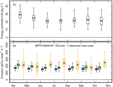
The staff and facilities at the research farm provided the herd management and automated individual measurements of milk yield and body weight at each milking. Milk was sampled individually 1 day per week and analyzed for its main components. Monthly energy-corrected milk (ECM) yield of the cows was calculated from daily milk yield and the contents of fat, protein, and lactose (Arrigo et al., 1999). Monthly ECM yield decreased over the first 3 months but overall it was fairly constant in time with a mean value of 22.7 kg and a standard deviation (SD) of 5.5 kg. The average live weight of 640 kg (SD 70 kg) slightly increased by around 6 % over the grazing season.
Wind speed
[m s1]
0 - 0.5 0.5 - 1 1 - 1.5 1.5 - 2 2 - 2.5 2.5 - 3 3 - 4 4 - 5 5 - 7.5 7.5 - 10
−100 −50 0 50 100 150
[m]
−
100
−
50
0
50
100
150
[m]
FARM FACILITIES
FARM FACS.
cereals
pasture
pasture
meado
w
PAD1
PAD2
PAD3
PAD4
PAD5
PAD6
−100 −50 0 50 100 150
EC tower
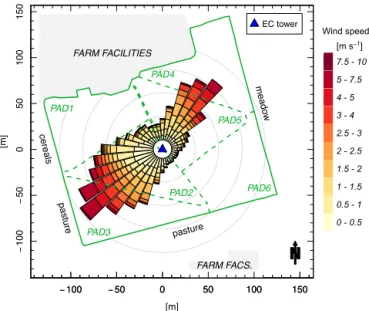
Figure 1.Plan of the measurement site with the pasture (solid green
line) and its division into six paddocks, PAD1 to PAD6 (dashed green lines), used for rotational grazing. Around the EC tower in the center, the wind direction distribution for the year 2013 is
in-dicated with a resolution of 10◦. The gray circles indicate sector
contributions of 2, 4, 6, and 8 % (from inside outwards). Each sec-tor is divided into color shades indicating the occurrence of wind speed classes (see legend).
barn and air temperature. If there was a risk of frost, the cows stayed in the barn overnight (58 nights), and if the daytime air temperature exceeded about 28◦C before noon, the cows
were moved into the barn for shade (19 days). Waterlogged soil condition entirely prohibited grazing on the pasture be-tween 12 and 13 April. In total the cows were grazing on the study field for 198 half-days and for another 157 half-days on nearby pastures not measured by the EC tower.
The management of the neighboring fields is also indicated in Fig. 1. The pastures in the southwest are the additionally used areas due to fodder shortage of the experimental site (see above) and were only used with cows participating in the experiment. The feeding behavior of each cow was mon-itored by RumiWatch (Itin+Hoch GmbH, Switzerland) hal-ters with a noseband sensor. From the pressure signal time se-ries induced by the jaw movement of the cow (Zehner et al., 2012) the relative duration of three activity classes (eating, ruminating, and idling) was determined using the converter software V0.7.3.2.
2.2 Eddy covariance measurements 2.2.1 Instruments and setup
The EC measurement tower was placed in the middle of the pasture and was enclosed by a two-wire electric fence to avoid animal interference with the instruments (Fig. 1). The 3-D wind vector components u, v (horizontal), andw
(vertical), as well as temperature were measured by an ultra-sonic anemometer (Solent HS-50, Gill Instruments Ltd., UK) mounted on a horizontal arm on the tower, 2 m above ground level. Methane, CO2, and water vapor concentrations were
measured with the cavity-enhanced laser absorption tech-nique (Baer et al., 2002) using a fast greenhouse gas ana-lyzer (FGGA; Los Gatos Research Inc., USA). The FGGA was placed in a temperature-conditioned trailer at 20 m dis-tance (NNE) from the EC tower and was operated in high-flow mode at 10 Hz. A vacuum pump (XDS35i Scroll Pump, Edwards Ltd., UK) pulled the sample air through a 30 m long PVC tube (8 mm ID) and through the analyzer at a flow rate of about 45 SLPM. The inlet of the tube was placed slightly below the center of the sonic anemometer head at a hori-zontal distance of 20 cm. Two particle filters with liquid wa-ter traps (AF30 and AFM30, SMC Corp., JP) were included in the sample line. The 5 µm air filter (AF30), installed 1 m away from the inlet, avoided contamination of the tube walls. The micro air filter (AFM30; 0.3 µm) was installed at the an-alyzer inlet.
The noise level of the FGGA for fast CH4measurements
depended on the cleanness of the cavity mirrors. It was de-termined as the (weekly) minimum of the half-hourly stan-dard deviation of the 10 Hz signal. At the beginning, the noise level was at 15 ppb but gradually increased to 38 ppb over time due to progressive contamination. In July 2013 the noise abruptly increased without any explanation, but clean-ing had to be postponed until mid-August. Durclean-ing this period the noise level was 230 to 400 ppb. After cleaning, the noise was even lower (around 7 ppb) than at the beginning.
The gas analyzer was calibrated at intervals of approxi-mately 2 months with two certified standard gas mixtures (1.5 ppm CH4/350 ppm CO2 and 2 ppm CH4/500 ppm
CO2; Messer Schweiz AG, Switzerland). The standard gas
was supplied with an excess flow via a T-fitting to the de-vice which was set at low measurement mode at 1 Hz using the internal pump. The calibration showed that the instru-ment sensitivity did not vary significantly over time, except for the period when the measurement cell was very strongly contaminated.
The data streams of the sonic anemometer and the dry air mixing ratios from the FGGA instrument were synchronized in real-time by a customized LabView (LabView 2009, Na-tional Instruments, USA) program and stored as raw data in daily files for offline analysis.
Standard weather parameters were measured by a cus-tomized automated weather station (Campbell Scientific Ltd., UK).
2.2.2 Flux calculation
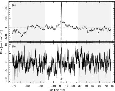
Figure 2.10 Hz time series of CH4mixing ratio for two exemplary 30 min intervals on 15 June 2013 between 12:30 and 14:30 local
time(a)with and(b)without cows in the FP. In black, untreated
data; in orange, data after de-spiking. The two cases correspond to the cross-covariance functions in Fig. 3a and b.
and temperature) were subject to a de-spiking (“soft flags”) routine according to Schmid et al. (2000); replacing val-ues that exceed 3.5 times the standard deviation within a running time window of 50 s. Filtered values were counted and replaced by a running mean over 500 data points. No de-spiking was applied for the CH4mixing ratio because a
potentially large effect on resulting fluxes was found. For cases with cows in the FP, the CH4 concentration showed
many large peaks as illustrated in Fig. 2a, whereas for con-ditions without cows the variability range was much lower (Fig. 2b). When the de-spiking routine is applied to the time series, this has a strong effect in the case with cows in the FP (Fig. 2a). In this 30 min interval, 454 data points are re-placed and the remaining concentration data are limited to 3500 ppb. The corresponding flux is reduced from 1322 to 981 nmol m−2s−1(−26 %). The second time series not
in-fluenced by cows shows no distinct spikes and only five data points are removed by the de-spiking routine without sig-nificant effect on the resulting flux. Prior to the covariance calculation, the wind components were rotated with the dou-ble rotation method (Kaimal and Finnigan, 1994) to align the wind coordinate system into the mean wind direction, and the scalar variables were linearly detrended.
The EC flux is defined as the covariance between the ver-tical wind speed and the trace gas mixing ratio (Foken et al., 2012b). Due to the tube sampling of the FGGA instrument there is a lag time between the recording of the two quanti-ties. Therefore, the CH4flux was determined in a three-stage
procedure: (i) for all 30 min intervals, the maximum absolute value (positive or negative) of the cross-covariance function and its lag position (“dynamic lag”) was searched for within a lag time window of±50 s; (ii) the “fixed lag” was determined as the mode (most frequent value) of observed dynamic lags over several days allowing for longer-term temporal changes due to the FGGA operational conditions; (iii) for the final data set, the flux at the fixed lag was taken if the deviation between the dynamic and the fixed lag was larger than 0.36 s
−500
0
500
1000
τfix (a)
−10
−5
0
5
10
Flux [nmol
m
−
2s
−
1]
τfix (b)
−70 −50 −30 −10 0 10 20 30 40 50 60 70 80
Lag time τ [s]
Figure 3.Cross-covariance function of CH4fluxes for two 30 min
intervals of 15 June 2013(a)with and(b)without cows in the
foot-print. The panels correspond to the intervals in Fig. 2.τfixindicates
the expected fixed lag time for the EC system. The gray areas on both sides indicate the ranges used for estimating the flux uncer-tainty and detection limit.
else the flux at the dynamic lag was taken. The fixed lag for the CH4flux in this study was around 2 s.
For large emission fluxes with cows in the FP, a pro-nounced and well-defined peak in the cross-covariance func-tion could be found close to the expected lag time (Fig. 3a). For small fluxes, the peak may be hidden in the random-like noise of the cross-covariance function and the maximum value may be found at an implausible dynamic lag position (Fig. 3b). In this case, the flux at the fixed lag is more repre-sentative on statistical average because it is not biased by the maximum search.
The air transportation through the long inlet tube (30 m) and the filters led to high-frequency loss in the signal (Fo-ken et al., 2012a). To determine the damping factor, suf-ficient flux intervals with good conditions are needed, i.e., cases with a large significant flux and very stationary condi-tions resulting in a well-defined cospectrum and ogive with a low noise level. These requirements were generally fulfilled better for CO2than for CH4fluxes. Because both quantities
were measured by the same device, we assumed that CH4
fluxes had the same high-frequency loss as determined for the more significant CO2 fluxes. High-frequency loss was
de-pending mainly on wind speed, was found for the presented setup, and the fluxes were corrected for this effect.
The mixing ratios measured by the FGGA were internally corrected for the amount of water vapor (at 10 Hz) and stored as “dry air” values. Since temperature fluctuations are sup-posed to be fully damped by the turbulent flow (Reynolds number of 10 000) in the long inlet line, no further correc-tion for correlated water vapor and temperature fluctuacorrec-tions (Webb, Pearman, and Leuning (WPL) density correction, Webb et al., 1980) was necessary.
2.2.3 Detection limit and flux quality selection
The flux detection limit was determined by analyzing the cross-covariance function of fluxes dominated by general noise, i.e., fixed lag cases without significant covariance peaks. Additionally, the selection was limited to smaller fluxes (in the range around zero for which more fixed lag than dynamic lag cases were found, here±26 nmol m−2s−1)
in order to exclude cases with unusually high non-stationarity effects. The uncertainty of the noise dominated fluxes was determined from the variability (standard deviation) of two 50 s windows on the left and the right side of the covariance function (Fig. 3) similar to Spirig et al. (2005). The detection limit was determined as 3 times the average of these standard deviations.
All measured EC fluxes were selected using basic quality criteria. The applied limits were chosen based on theoretical principles and statistical distributions of the tested quantities. Only cases which fulfilled the following criteria were used for calculations:
– less than 10 hard flags in wind and concentration time series,
– small vertical vector rotation angle (tilt angle) within
±6◦to exclude cases with non-horizontal wind field,
– wind direction within sectors 25 to 135◦and 195 to 265◦
to exclude cases that were affected by the farm facili-ties to the north and to the south of the study field (by non-negligible flux contribution, non-stationary advec-tion, distortion of wind field, and turbulence structure), – fluxes above the detection limit need a significant
co-variance peak (dynamic lag determination).
Moving sources in the FP lead to strong flux variations which are normally identified by the stationarity criterion (Foken et al., 2012a). We did not apply a stationarity test because it would have potentially removed cases with high cow contri-butions. We also did not apply a u∗ threshold filter that is often used for CO2flux measurements (Aubinet et al., 2012)
because it would have been largely redundant with the other applied quality selection criteria (with a negligible effect of
<2 % on mean emissions). Table 1 shows the reduction in number of fluxes due to the quality selection criteria.
2.3 GPS method for deriving animal CH4emission To assess the reliability of EC flux measurements of CH4
emissions by cows on the pasture, the measured fluxes (FEC)
had to be converted to average cow emissions (E) per animal and time. This was done using three different information levels about animal position and distribution on the pasture:
1. GPS method: use of time-resolved position for each an-imal from GPS cow sensors (this section),
2. PAD method: use of detailed paddock stocking time schedule (Sect. 2.4),
3. FIELD method: using only the seasonal average stock-ing rate on the measurement field without stockstock-ing schedule details (Sect. 2.5).
2.3.1 Animal position tracking
For animal position tracking, each cow was equipped with a commercial hiking GPS device (BT-Q1000XT, Qstarz Ltd., Taiwan) attached to a nylon web halter at the cows neck to optimize satellite signal reception. The GPS loggers using the WAAS, EGNOS, and MSAS correction (Witte and Wil-son, 2005) continuously recorded the position at a rate of 0.2 Hz. Each GPS device was connected to a modified tery pack with three 3.6 V lithium batteries to extend the bat-tery lifetime up to 10 days. GPS data were collected from the cow sensors weekly during milking time, and at the same occasion also the batteries were exchanged. GPS co-ordinates were transformed from the World Geodetic System (WGS84) to the metric Swiss national grid (CH1903 LV95) coordination system. GPS data were filtered for cases with low quality depending on satellite constellation (positional dilution of precision PDOP≤5). Each track was visually in-spected for malfunction to exclude additional bad data not excluded by the PDOP criterion. Smaller gaps (<1 min) in the GPS data of individual cow tracks were linearly inter-polated. The total coverage of available GPS data was used as a quality indicator for each 30 min interval. The position data were used to distinguish between 30 min intervals when the cows were on the study field or elsewhere (barn or other pasture), or moving between the barn and the pasture.
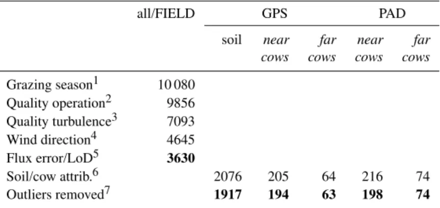
Table 1.Number of available 30 min CH4fluxes in this study after the application of selection criteria for the three calculation methods (FIELD, GPS, and PAD method). Bold numbers were used for final calculations.
all/FIELD GPS PAD
soil near far near far
cows cows cows cows
Grazing season1 10 080
Quality operation2 9856
Quality turbulence3 7093
Wind direction4 4645
Flux error/LoD5 3630
Soil/cow attrib.6 2076 205 64 216 74
Outliers removed7 1917 194 63 198 74
1Total number of 30 min intervals in grazing season (9 April–4 April 2013). 2Available data with proper instrument operation (hard flags<10).
3Acceptable quality of turbulence parameters and vertical tilt angle within±6◦.
4Accepted (undisturbed) wind direction: 25 to 135◦and 195 to 265◦. 5No fluxes at fixed lag if flux larger than flux detection limit (LoD).
6Split fluxes based on GPS data; exclusion of intervals with low GPS data coverage; exclusion of
intervals (730) when cows were being moved between barn and pasture; discarding of cases with intermediate mean cow FP weights.
7Outliers for cow cases determined based on emissions (Ecow).
for individual GPS sensors occurred during the continuous operation, the overall data coverage was satisfactory for sen-sors attached to animals. Time intervals with less than 70 % of cow GPS positions available, were discarded from the data evaluation. This occurred in only 8 % of the cases.
2.3.2 Footprint calculations
An EC flux measurement represents a weighted spatial aver-age over a certain upwind surface area called flux FP. The FP weighting function can be estimated by dispersion models. Kormann and Meixner (2001) published a FP model (KM01) based on an analytical solution of the advection–dispersion equation using power functions to describe the vertical pro-files. The basic Eq. (1) describes the weight functionϕof the
relative contribution of each upwind location to the observed flux with thexcoordinate for longitudinal andy coordinate for lateral distance.
ϕ (x, y)=√ 1
2π·D·xEe
−y2 2·(D·xE)2
·C·x−A·e−xB (1)
The termsAtoEare functions of the necessary micrometeo-rological input parameters (z−d: aerodynamic height of the flux measurement;u∗: friction velocity;L: Monin–Obukhov length;σv: standard deviation of the lateral wind component;
wd: wind direction;u: mean wind speed) which were mea-sured by the EC system.
The FP weight function also needs the aerodynamic rough-ness length (z0) as input parameter. It can be calculated as
described in Neftel et al. (2008) from the other input param-etersz−d,u∗,L, anduby solving the following wind profile
relationship:
u (z−d)=u∗
k
ln
z
−d
z0
−ψH
z
−d
L
. (2)
However, the determination ofz0with this equation is
sen-sitive to the quality of the other parameters and especially problematic in low-wind conditions with relatively high un-certainty in the measuredu∗. Becausez0 is considered
ap-proximately constant for given grass canopy conditions, its average seasonal course for the measurement field was pa-rameterized by fitting a polynomial to individual results of Eq. (2) which fulfilled the following criteria:u >1.5 m s−1
(see e.g., Graf et al., 2014), days without snow cover, and mean wind direction in the undisturbed sectors 25 to 135◦
and 195 to 265◦(other wind direction showed relatively large
variation ofz0).
Because of short-term variability in the vegetation cover and because of the potential impact of cows onz0, a range of
a factor of 3 on both sides of the fitted parameterization (see Fig. 7) was defined. If the individual 30 minz0value (derived
with Eq. 2) was within this range, it was directly used for the FP calculation. Ifz0exceeded this range it was restricted to
the upper/lower bound of the range.
Assuming that each cow represents a (moving) point source of CH4, the FP contribution of each 5 s cow position
(Fig. 4a) was calculated according to Eq. (1). The individ-ual values were then averaged for each 30 min interval to the mean FP weight of a cowϕcow and of the entire cow herd
ϕherd:
ϕherd=ncow·ϕcow=ncow·
"
1 N
N
X
i=1
ϕ (xi, yi)
#
withncowdenoting the number of cows in the herd, andNthe
total number of available GPS data points within the 30 min interval. To account for the uncertainty of the GPS position, each data point was blurred by adding 4 m in each direction from the original point.ϕ(xi, yi) was calculated as the mean
of the five ϕ(x, y). Values of ϕherd were accepted only for 30 min intervals where >70 % of the GPS data was avail-able and the input parameters L,u∗, andσv were of
suffi-cient quality. According to Eq. (3) it was assumed implic-itly that the FP weight of the cows with missing GPS data corresponded to the mean weight of the cows with available position data.
2.3.3 Calculation of average cow emission
The measured flux (FEC) cannot be entirely attributed to the
contribution of direct cow emissions within the FP. It also includes the CH4exchange flux of the pasture soil
(includ-ing the excreta patches). This contribution is denoted as “soil flux” (Fsoil) in the following.Fsoilhad to be quantified by
se-lecting fluxes with no or negligible influence of cows based on the GPS FP evaluation and other selection criteria (Ta-ble 1).
The GPS data allows for the calculation of emissions based on actual observed cow distribution and the use of the aver-age herd FP weights (Eq. 3). The averaver-age emission per cow (Ecow) for a 30 min interval is determined as
Ecow= (FECϕ−Fsoil)
herd
. (4)
In addition to the quality selection criteria for the EC fluxes mentioned in Sect. 2.2.3, theEcowand theFsoildata sets were
subject to an outlier test and removal. Outliers were identified using the box plot function of R (R Core Team, 2014) as values with a distance from the box (inter-quartile rage) of greater than 1.5 times the length of the box. The effect of the outlier removal on the number of available data is indicated in Table 1.
2.4 PAD method for deriving animal CH4emission To assess the effect of the precision of cow position infor-mation on the determination of the average cow emission, an option with less detailed but easier to obtain position infor-mation was also applied and compared to the GPS approach. In the PAD method, no individual cow position informa-tion is used, but it is assumed that the animal CH4 source
is evenly distributed over the occupied paddock area. For this approach, an accurate paddock stocking time schedule is needed.
2.4.1 Footprint calculation for paddocks
Neftel et al. (2008) developed a FP tool based on Eq. (1) that calculates the FP weights of quadrangular areas upwind of an EC tower. The source code was adapted and transferred
−100 −50 0 50
[m] − 100 − 50 0 [m] ● ● ● ● ● ● ● ● ● ● ● ● ● ● ● ● ● ● ● ● ● ● ● ● ● ● ● ● ● ● ● ● ● ● ● ● ● ● ● ● ● ● ● ● ● ● ● ● ● ● ● ● ● ● ● ● ● ● ● ● ● ●●●● ● ● ●●●●●●●●● ●●●●●●●●●● ● ● ● ● ● ● ● ● ● ● ● ● ● ● ● ● ● ● ● ●●●●●●●●●●●●●●●●● ●●●●●●●●●●●●●●●●●●●●●●● ● ● ● ● ● ●●●● ● ● ● ● ● ● ● ● ● ● ● ● ● ● ● ● ● ● ● ● ● ● ● ● ● ● ● ● ● ● ● ● ● ● ● ● ● ● ● ● ● ● ● ● ● ● ● ● ● ● ● ● ● ● ● ● ● ● ● ● ● ● ● ● ● ● ● ● ● ● ● ● ● ● ● ● ● ● ● ● ● ● ● ● ● ● ● ● ● ● ● ● ●●●●● ● ● ● ● ● ● ● ● ● ● ● ● ● ● ● ● ● ● ● ● ● ● ● ● ● ● ● ● ● ● ● ● ● ● ● ● ● ● ● ● ● ● ● ● ● ● ● ● ● ● ● ● ● ● ● ● ● ● ● ● ● ● ● ● ● ● ● ● ● ● ● ● ● ● ● ● ● ● ● ● ● ● ● ● ● ● ● ● ● ● ● ● ● ● ● ● ● ● ● ● ● ● ● ● ● ● ● ● ● ● ● ● ● ● ● ● ● ● ● ● ● ● ● ● ● ● ● ● ● ● ● ● ● ● ● ● ● ● ● ● ● ●●●●●●●●●●●●●●●●●●●●●●●●●●●●●●●●●●●●●●●●●●●●●●●●●●●●●●●●●●●●●●●●●●●●●●●●●●●●●●●●●●●●●●●●●●●●●●●●●●●●●●●●●●●●●●●●●●●●●●●●●●●●●●●●●●●●●●●●●●●●●●●●●●●●●●●●●●●●●●● ● ● ● ● ●● ●●●●●●●●●●●●●●●●●●●●●●●●●●●●●●●●●●●●●●●●●●●●●●●●●●●●●●●●●●●●●●●●●●●●●●●●●●●●●●●●●●●●●●●●●●●●●●●●●●●●●●●●●●●●●●●●●●●●●●●●●●●●●●●●●●●●●●●●●●●●●●●●●●●●●●●●●●●●●●●●●●● ● ● ● ● ● ● ● ● ● ● ● ● ● ● ● ● ● ● ● ● ● ● ● ● ● ● ● ● ● ● ● ● ● ● ● ● ● ● ● ● ● ● ● ● ● ● ● ● ● ● ● ● ● ● ● ● ● ● ● ● ● ● ● ● ● ● ● ● ● ● ● ● ● ● ● ● ● ● ● ● ● ● ● ● ● ● ● ● ● ● ● ● ● ● ● ● ● ● ● ● ● ● ● ● ● ● ● ● ● ● ● ● ● ● ● ● ● ● ● ● ● ● ● ● ● ● ● ● ● ● ● ● ● ● ● ● ● ●●●●●●●●●●●●●●●●●●●●●●●●●●●●●●●●●●●●●●●●●●●●●●●●●●●●●●●●●●●●●●●●●●●●●●●●●●●●●●●●●●●●●●●●●●●●●●●●●●●●●●●●●●●●●●●●●●●●●●●●●●●●●●●●●●●●●●●●●●●●●●●●●●●●●●●●●●●●●●●●●●●●●●●●●●●●●●●●●●●●●●●●●●●●●●●●●●●●●●●●●●●●●●●●●●●●● ● ● ● ● ● ● ● ● ● ● ● ● ● ● ● ● ● ● ● ● ● ● ● ● ● ● ● ● ● ● ● ● ● ● ● ● ● ● ● ● ● ● ● ● ● ● ● ● ● ● ●●●●●●●●●●●●●●●●●●●●●●●●●●●●●●●●●●●●●●●●●●●●●●●●●●●●●●●●●●●●●●●●●●●●●●●●●●●●●●●●●●●●●●●●●●●●●●●●●●●●●●●●●●●●●●●●●●●●●●●●●●●●●●●●●●●●●●●●●●●●●●●●●●●●●●●●●●●●●●●●●●●●●●●●●●●●●●●●●●●●●●●●●●●●●●●●●●● ● ● ● ● ● ● ● ● ● ● ● ● ● ● ● ● ● ● ● ● ● ● ● ● ● ● ● ● ● ● ● ● ● ● ● ● ● ● ● ● ● ● ● ● ● ● ● ● ● ● ● ● ● ● ● ● ● ● ● ● ● ● ● ● ● ● ● ● ● ● ● ● ● ● ● ● ● ● ● ● ● ● ● ● ● ● ● ● ● ● ● ● ● ● ● ● ● ● ● ● ● ● ● ● ● ● ● ● ● ● ● ● ● ● ● ● ● ● ● ● ● ● ● ● ● ● ● ● ● ● ● ● ● ●●●●●●●●●●●●●●●●●● ● ● ● ●●●●●●●●●●●●●●●●●●●●●●●●●●●●●●●●●●●●●●●●●●●●●●●●●●●●●●●●●●●●●●●●●●●●●●●●●●●●●●●●●●●●●●●●●●●●●●●●●●●●●●●●●●●●● ● ● ● ● ● ● ● ● ● ● ● ● ● ● ● ● ● ● ● ●● ● ● ● ● ● ● ● ● ● ● ● ● ● ● ● ● ● ● ● ● ● ● ● ● ● ●●●●●●●●●●●●● ● ● ● ● ● ● ● ● ● ● ● ● ● ● ● ● ● ● ● ●●●●●●●●●●●●●● ● ● ● ● ● ● ● ●●● ● ●●●●●●●●●●●●●●●●●●●●●●●●● ● ● ● ● ● ● ● ● ● ● ● ● ● ● ● ● ● ● ● ● ● ●●●● ●●● ●●●●● ● ● ● ● ● ●●●●●●●●●●●●●●●●●●●●●●●●●●●●●●●●●●●●●●●●●●●●●●●●●●●●●●●● ● ● ● ● ● ● ● ● ● ● ● ● ● ● ● ● ● ● ● ● ● ● ● ● ● ● ● ● ● ● ● ● ● ● ● ● ● ● ● ● ● ● ● ● ● ● ● ● ● ● ● ● ● ● ● ● ● ● ● ● ● ● ● ● ● ● ● ● ● ● ● ● ● ● ● ● ● ● ● ● ● ● ● ● ● ● ● ● ● ● ● ● ● ● ● ● ● ● ● ● ● ● ● ● ● ● ● ● ● ● ● ● ● ● ● ● ● ● ● ● ● ● ● ● ● ● ● ● ● ● ● ● ● ● ● ● ● ● ● ● ● ● ● ● ● ● ● ● ● ● ● ●●●●●●●●●●●●●●●●●●●●●●●●●●●●●●●●●●●●●●●●●●●●●●●●●●●●●●●●●●●●●●●●●●●●●●●●●●●●●●●●●●●●●●●●●●●●●●●●●●●●●●●●●●●●●●●●●●●●●●●●●●●●●●●●●●●●●●●●●●●●●●●●●●●●●●●●●●●●●●●●●●●●●●●●●●●●●●●●●●●●●●●●●●●●●●●●●●●●●●●●●●●●●●●●● ● ● ● ● ● ● ● ● ● ● ● ●● ● ● ●●● ● ● ● ● ● ● ● ● ● ● ● ● ● ● ● ● ●●●●●●●●●●●●●●●●●●●●●●●●●●●●●●●●●●●●●●●●●●●●●●●●●●●●●●●●●●●●●●●●●●●●●●●●●●●●●●●●●●●●●●●●●●●●●●●●●●●●●●●●●●●●●●●●●●●●●●●●●●●●●●●●●●●●●●●●●●●●●●●●●●●●●●●●●●●●●●●●●●●●●●●●●●●●●●●●●●●●●●●●●●●●●●●●●●●●●●●●●●●●●●●●●●●●●●●●●●●●●●●●●●●●●●●●●●●●●●●●●●●●●●●●●●●●●●●●●●●●●●●●●●●●●●●●●●●●●●●● ● ● ● ● ● ● ● ● ● ● ● ● ● ● ● ● ● ● ● ● ● ● ● ● ● ● ● ● ● ● ● ● ● ● ● ● ● ● ● ● ● ● ● ● ● ● ● ● ● ● ● ● ● ● ● ● ● ● ● ● ● ● ● ● ● ● ● ● ● ● ● ● ● ● ● ● ● ● ● ● ● ● ● ● ● ● ● ● ● ● ● ● ● ● ● ● ● ● ● ● ● ● ● ● ● ● ● ● ● ● ● ● ● ● ● ● ● ● ● ● ● ● ● ● ●●●●●●●●● ● ● ● ● ●●●●●●●●●●●●●●●●●●●●●●●●●●●●●●●●●●●●●●●●●●●●●●●●●●● ●● ● ● ● ● ● ● ● ● ● ● ● ●● ● ● ● ● ● ● ● ● ● ● ● ● ● ● ● ● ● ● ● ● ● ● ● ● ● ● ● ●●●●●●● ● ● ● ●●●●●●●●●●●●●●●●●●●●●●●●●●●●●●●●●●●●●●●●●●●●●●●●●●●●●●●●●●●●●●●●●●●●●●●●●●●●●●●●●●●●●●●●●●●●●●●●●●●●●●●●●●●●●●●●●●●●●●●●●●●●●●●●●●●●●●●●●●●●●●●●●●●●●●●●●●●●●●●●●●●●●● ● ● ● ● ● ● ● ● ● ● ● ● ● ● ● ● ● ● ● ● ● ● ● ● ● ● ● ● ● ● ● ● ● ● ● ● ● ● ● ● ● ● ● ● ● ● ● ● ● ● ● ● ● ● ● ● ● ● ● ● ● ● ● ● ● ● ● ● ● ● ● ● ● ● ● ● ● ● ● ● ● ● ● ● ● ●●●●● ● ● ● ● ● ● ● ● ● ● ●●●●●●●●●●●●●●●●●●●●●●●●●●●●●●●●●●●●●●●●●●●●●●●●●●●●●●●●●●●●●●●●●●●●●●●●●●●●●●●●●●●●●●●●●●●●●●●●●●●●●●●●●●●●●● ● ● ● ● ● ● ●● ● ● ● ● ● ● ● ● ● ● ● ● ● ● ● ● ● ● ● ● ● ● ● ● ●● ● ● ● ● ● ● ● ● ● ● ● ● ● ● ● ● ● ● ● ● ● ● ● ● ● ● ● ● ● ● ● ● ● ● ● ●● ● ● ● ●●●●●● ● ● ● ● ● ● ●●●●●●●●●●●●●● ● ● ●●●●● ● ● ● ● ●●● ●●●●●●●●●●●●●●●●●●●●●●●●●●●●●●●●●●●● ● ● ● ● ● ● ● ● ● ● ● ● ● ● ● ● ● ● ● ● ● ● ● ● ● ● ● ● ● ● ● ● ● ● ● ● ● ● ● ● ● ● ● ● ● ● ● ● ● ● ● ● ● ● ● ● ● ● ● ● ● ● ● ● ● ● ● ● ● ● ● ● ● ● ● ● ● ● ● ● ● ● ● ● ● ● ● ● ● ● ● ● ● ● ● ● ● ● ● ● ● ● ● ● ● ● ● ● ● ● ● ● ● ● ● ● ● ● ● ● ● ● ● ● ● ● ● ● ● ● ● ● ● ● ● ● ● ● ● ● ● ● ● ● ● ● ● ● ● ● ● ● ● ● ● ● ● ● ● ● ● ● ● ● ● ● ● ● ● ● ● ● ● ● ● ● ● ● ● ● ● ● ● ● ● ● ● ● ● ● ● ● ● ● ● ● ● ● ● ● ● ● ● ● ● ● ● ● ● ● ● ● ● ● ● ● ● ● ● ● ● ● ● ● ● ● ● ● ● ● ● ● ● ● ● ● ● ● ● ● ● ● ● ● ● ● ● ● ● ● ● ● ● ● ● ● ● ● ● ●●●●●● ● ● ● ● ● ● ● ● ● ● ● ● ● ● ● ● ● ● ● ● ● ● ● ● ● ● ● ● ● ● ● ● ● ● ● ● ● ● ● ● ● ● ● ● ● ● ● ● ● ● ● ● ● ● ● ● ● ● ● ● ● ● ● ● ● ● ● ● ● ● ● ● ● ● ● ● ● ● ● ● ● ● ● ● ● ● ● ● ● ● ● ● ● ● ● ●●●●●●●●●●●●●●●●●●●●●●●●●●●●●●●●●●●●●●●●●●●●●●●●●●●●●●●●●●●●●●●●●●●●●●●●●●●●●●●●●●●●●●●●●●●●●●●●●●●●●●●●●●●●●●●●●●●●●●●●●●●●●●●●●●●●●●●●●●●●●●●●●●●●●●●●●●●●●●●●●●●●●●●●●●●●●●●●●●●●●●●●●●●●●●●●●●●●●●●●●●●●●●●●●●●●●●●●●●●●●●●●●●●●●●●●●●●●●●●●●●●●●●●●●●●●●●●●●●●●●●●●●●●●●●●●●●●●●●●●●●●●●●●●●●●●●●●●●●●●●●●●●●●●●●●●●●●●●●●●●●●●●●●●●●●●●●●●●●●●●●●●●●●●●●●●●●●●●●●● ● ● ● ● ● ● ● ● ● ● ● ● ● ● ● ● ● ● ● ● ● ● ● ● ● ● ● ● ● ● ● ● ● ● ● ● ● ● ● ● ● ● ● ● ● ● ● ● ● ● ● ● ● ● ● ● ● ● ● ● ● ● ● ● ● ● ● ● ● ● ● ● ● ● ● ● ● ● ● ● ● ● ● ● ● ● ● ● ● ● ● ● ● ● ● ● ● ● ● ● ● ● ● ● ● ● ● ● ● ● ● ● ● ● ● ● ● ● ● ● ● ● ● ● ● ● ● ● ● ● ● ● ● ● ● ● ● ● ● ● ● ● ● ● ● ● ● ● ● ● ● ● ● ● ● ● ● ● ● ● ● ● ● ● ● ● ● ● ● ● ● ● ● ● ● ● ● ● ● ● ● ● ● ● ● ● ● ● ● ● ● ● ● ● ● ● ● ● ● ● ● ● ● ● ● ● ● ● ● ● ● ● ● ● ● ● ● ● ● ● ● ● ● ● ● ● ● ● ● ● ● ● ● ● ● ● ● ● ● ● ● ● ● ● ● ● ● ● ● ● ● ● ● ● ● ● ● ● ● ● ● ● ● ● ● ● ● ● ● ● ● ● ● ● ● ● ● ● ● ● ● ● ● ● ● ● ● ● ● ● ● ● ● ● ● ● ● ● ● ● ● ● ● ● ● ● ● ● ● ● ● ● ● ● ● ● ● ● ● ● ● ● ● ● ● ● ● ● ● ●●●●●●●●●●●●●●●●●●●●●●●●●●●●●●● ● ● ● ● ● ● ● ● ● ● ● ● ● ● ● ● ● ● ● ● ● ● ● ● ● ● ● ● ● ● ● ● ● ● ● ● ● ● ● ● ● ● ● ● ● ● ● ● ● ● ● ● ● ● ● ● ● ● ● ● ● ● ● ● ● ● ● ● ● ● ● ● ● ● ● ● ● ●●●●●●●●●●●●●●●●●●●●●●●●●●●●●●●●●●●●●●●●●●●●●●●●●●●●●●●●●●●●●●●●●●●●●●●●●●●●●●●●●●●●●●●●●●●●●●●●●●●●●●●●●●●●●●●●●●●●●●●●●●●●●●●●●●●●●●●●●●●●● ● ●●● ● ● ● ● ● ● ● ● ● ● ● ● ● ● ● ● ● ● ● ● ●●●●●●●●●●●●●●●●●●●●●●●●●●●●●●●●●●●●●●●●●●●●●●●●●●●●●●●●●●●●●●●●●●●●●●●●●●●●●●●●●●●●●●●●●●●●●●●●●●●●●●●●●●●●●●●●●●●●●● ● ● ● ● ● ● ● ● ● ● ●●●●●●●●●●●●●●●●●●●●●● ●●●●●●●●●●●● ● ● ● ● ● ● ● ● ● ● ● ● ● ● ●● ● ● ● ● ● ●●●●●●●●●●●●●●●●●●●●●●●●●●●●●●●●●●●●●●●●●●●●●●●●●●●●●●●●●●●●●●●●●●●●●●●●●●●●●●●●●●●●●●●●●●●●●●●●●●●●●●●●●●●●●●●●●●●●●●●●●●●●●●●●●●●●●●●●●●●●●●●●●●●●●●●●●●●●●●●●●●●●●●●●●●●●●●●●●●●●●●●●●●●●●●●●●●●●●●●●●●●●●●●●●●●●●●●●●●●●●●●●●●●●●●●●●●●●●●●●●●●●●●●●●●●●●●●●●●●●●●●●●●●●●●●●●●●●●●●●●●●●●●●●●●●●●●● ● ● ● ● ● ● ● ● ● ● ● ● ● ● ● ● ● ● ● ● ● ● ● ● ● ● ● ● ● ● ● ● ● ● ● ● ● ● ● ● ● ● ● ● ● ● ● ● ● ● ● ● ● ● ● ● ● ● ● ● ● ● ● ● ● ● ● ● ● ● ● ● ●●● ● ● ● ●●●●● ● ● ●●●●●●●●●●●●●●●●●●●●●●●●●●●●●●●●●●●●●●●●●●●●●●●●●●●●●●●●●●●●●●●●●●●●●●●●●●●●●●●●●●●●●●●●●●●●●●●●●●●●●●●●●●●●●●●●●●●●●●●●●●●●●●●●●●●●●●●●●●●●●●●●●●●●●●●●●●●●●●●●●●●●●●●●●●●●●●●●●●●●●●●●●●●●●●●●●●●●●●●●●●●●●●●●●●●●●●●●●●●●●●●●●●●●●●●●●●●●●●●●●●●●●●●●●●●●●●●●●●●●●●●●●●●●●●●●●●● ● ● ● ● ● ● ● ● ● ● ● ● ● ● ● ● ● ● ● ● ●●●● ●● ●●●●●●●●●●●●●●●●●●●●●●●●●●●●●●●●●●●●●●●●●●●●●●●●●●●●●●●●●●●●●●●●●●● ● ● ● ● ● ● ● ● ● ● ● ● ● ● ● ● ● ● ● ● ● ● ● ● ●● ● ●●●●●●●●●●●●●●●●●●●●●●●●●●●●●●●●●●●●●●●●●●●●●●●●●●●●●●●●●●●●●●●●●●●●●●●●●●●●●●●●●●●●●●●●●●●●●●●●●●●●●●●●●●●●●●●●●●●●●●●●●●●●●●●●●●●●●●●●●●●●●●●●●●●●●●●●●●●●●●●●●●●●●●●●●●●●●●●●●●●●●●●●●●●●●●●●●●●●●●●●●●●●●●●●●●●●●●●●●●●●●●●●●●●●●●●●●●●●●●●● ● ● ● ● ● ● ● ● ● ● ● ● ● ● ● ● ●●● ● ● ● ● ● ● ● ● ●●●●●●●●●●●●● ● ● ● ● ● ● ● ● ● ● ● ● ● ● ● ● ● ● ● ● ● ● ● ● ● ● ● ● ● ● ● ● ● ● ● ● ●●● ● ● ● ● ● ● ● ● ● ● ● ● ● ● ● ● ● ● ● ● ● ● ● ● ● ● ● ● ● ● ●● ● ● ● ● ● ● ● ● ● ● ● ● ● ● ● ● ● ● ● ● ● ● ● ● ● ● ● ● ● ● ● ● ● ● ● ● ● ● ● ● ● ● ● ● ● ● ● ● ● ● ● ● ● ● ● ● ● ● ● ● ● ● ● ● ● ● ● ● ● ● ● ● ● ● ● ● ●●●●●●●●●●●●●●●●●●●●●●●●●●●●●●●●●●●●●●●●●●●●●●●●●●●●●●●●●●●●●●●●●●●●●●●●●●●●●●●●●●●●●●●●●●●●●●●●●●●●●●●●●●●●●●●●●●●●●●●●●●●●●●●●●●●●●●●●●●●●●●●●●●●●●●●●●●●●●●●●●●●●●●●●●●●●●
ϕherd = 0.0026 head m−2
(a) ϕ
x10−4
2.0 4.0 6.0 8.0
0
−100 −50 0 50
[m]
PAD2 PAD3
ΦPAD2 = 64%
ΦPAD3 = 23%
(b) ϕ
x10−4
2.0 4.0 6.0 8.0
0
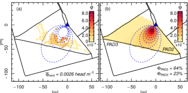
Figure 4.Determination of footprint weights for a cow herd in
PAD2 during a 30 min interval with two different approaches:
(a)GPS method (Eq. 3) based on the actual cow positions;(b)PAD
method (Eq. 5) calculating the area integrated footprint weight of
the entire paddock area (here8PAD2=64 %) with the resolution of
a 4×4 m grid. The reddish color scale indicates the footprint weight
of each location. The blue triangle indicates the position of the EC tower and the blue dashed lines are isolines of the footprint weight function.
to an R routine in order to allow for more complex polygons instead of quadrangles for the different sub-areas of interest (here paddocks).
Under the assumption that an observed flux originates from a known source and that the source is uniformly dis-tributed over a defined paddock area, the measured fluxes can be corrected with the integrated FP weight (Neftel et al., 2008):
8PAD=
Z Z
PAD area
ϕ (x, y) dxdy. (5)
In the FP tool, the domain which covers 99 % of the FP is divided into a grid of 200×100 (along-wind by crosswind) cells, and for each cell the FP weight is calculated. The sum of all cells lying in the area of interest is the FP weight of the area (Eq. 5 and Fig. 4b). The FP model had already been validated in a field experiment with a grid of artificial CH4
sources and two EC flux systems (Tuzson et al., 2010). 2.4.2 Determination of average cow emission
With the information on pasture time and occupied paddock number, the average cow emission for a 30 min interval is calculated as
Ecow= (FEC−8Fsoil)·APAD
PAD ·
1
ncow
, (6)
withncowdenoting the number of cows in the occupied
pad-dock,APADthe area, and8PADthe FP fraction of the
cor-responding paddock. Emissions are calculated only for the 30 min intervals where the cows were on the pasture, the FP weight of the grazed paddock8PADexceeds 0.1, and FP
− 100 − 50 0 50 100 150 [m]
FEC = 8.8 nmol m−
2 s−1
(a)
FEC = 633.6 nmol m−
2 s−1
(b)
−100 −50 0 50 100
[m] − 100 − 50 0 50 100 150 [m]
FEC = 263.5 nmol m−2 s−1
(c)
−100 −50 0 50 100
[m]
FEC = 3.1 nmol m−2 s−1
(d)
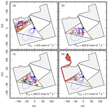
Figure 5.Four examples of 30 min intervals with similar wind and
footprint conditions (blue isolines) but different cow distribution
and observed fluxes (FEC). For each cow, the registered GPS
po-sition (5 s resolution over 30 min) is marked with a line of a
differ-ent color. Paddocks represdiffer-entingnear cowscases are white andfar
cowsare gray.(a)No cows in the footprint, i.e. soil fluxes are
mea-sured,(b–d)the higher the number and residence time of cows in
the footprint the larger the observed flux.
2.5 FIELD method for deriving animal CH4emission without position information
EC measurements are frequently performed over pastures, but usually no detailed information on the position and exact number of animals and specific occupation times are avail-able. If at least the average stocking rate over the grazing period is available and under the assumption that the cows are uniformly distributed over the entire pasture, the time-averaged cow emissions can be calculated as
hEcowi =(hFECi − hFsoili)·Afield· 1
hncowi, (7)
withhFECidenoting the mean observed CH4flux of the
graz-ing period,Afieldthe total pasture area, andhncowithe mean
number of cows on the study field over the grazing season.
hncowi =6.6 heads is calculated as the total number of cows of each 30 min interval with cows on the study field plus one-half of the number of cows when the cows were moved be-tween barn and pasture divided by the total number of 30 min intervals of the grazing period. For comparability reasons, the sameFsoilresults (selected based on GPS data) were used
for all three methods. It should be noted that an appropriate determination of the soil flux may be difficult without any cow position information.
● ● ● ● ● ● ● ● ● ● ● ● ● ● ● ● ● ● ● ● ● ● ● ● ● ● ● ● ●●● ● ● ● ● ● ● ● ● ● ● ● ● ● ● ● ● ● ● ● ● ● ● ● ● ● ● ● ● ● ● ● ● ● ● ● ● ● ● ● ● ● ● ● ● ● ● ● ● ● ●●● ● ● ● ● ● ● ● ● ● ● ● ● ● ● ● ● ● ● ● ● ● ● ● ● ● ● ● ● ● ● ● ● ● ● ● ● ● ● ● ● ● ● ● ● ● ● ● ● ● ● ● ● ● ● ● ● ● ● ● ● ● ● ● ● ● ● ● ● ● ● ● ● ● ● ● ● ● ● ● ● ● ● ● ● ● ● ● ● ● ● ● ● ● ● ● ● ● ● ● ● ● ● ● ● ● ● ● ● ● ● ● ● ● ● ● ● ● ● ● ● ● ● ● ● ● ● ● ● ● ● ● ● ● ● ● ● ● ● ● ●● ● ● ● ● ● ● ● ● ● ● ● ● ● ● ● ● ● ● ● ● ● ● ● ● ● ● ● ● ● ● ● ● ● ● ● ● ● ● ● ● ● ● ●● ● ● ● ● ● ● ● ● ● ● ● ● ● ● ● ● ● ● ● ● ● ● ● ● ● ● ● ● ● ● ● ● ● ● ● ● ● ● ● ● ● ● ● ● ● ● ● ● ● ● ● ● ● ● ● ● ● ● ● ● ● ● ● ● ● ● ● ● ● ● ● ● ● ● ● ● ● ● ● ● ● ● ● ● ● ● ● ● ● ● ● ● ● ● ● ● ● ● ● ● ● ● ● ● ● ● ● ● ● ● ● ● ● ● ● ● ● ● ● ● ● ● ● ● ● ● ● ● ● ● ● ● ● ● ● ● ● ● ● ● ● ● ● ● ● ● ● ● ● ● ● ● ● ● ● ● ● ● ● ● ● ● ● ● ● ● ● ● ● ● ● ● ● ● ● ● ● ● ● ● ● ● ● ● ● ●●● ● ● ● ● ● ●●● ● ● ● ● ● ● ● ● ● ● ● ● ● ● ● ● ● ● ● ● ● ● ● ● ● ● ● ● ● ● ● ● ● ● ● ● ● ● ● ● ● ● ● ● ● ● ● ● ● ● ● ● ● ● ● ● ● ● ● ● ● ● ● ● ● ● ● ● ● ● ● ● ● ● ● ●● ● ● ● ● ● ● ● ● ● ● ● ● ● ● ● ● ● ● ● ● ● ● ● ● ● ● ● ● ● ● ● ● ● ● ● ● ● ● ● ● ● ● ● ● ● ● ● ● ● ● ● ● ● ● ● ● ● ● ● ● ● ● ● ● ● ● ● ● ● ● ● ● ● ● ● ● ● ● ● ● ● ● ● ● ● ● ● ● ● ● ● ● ● ● ● ● ● ● ● ● ● ● ● ● ● ● ● ● ● ● ● ● ● ● ● ● ● ● ● ● ● ● ● ● ● ● ● ● ● ● ● ● ● ● ● ● ● ● ● ● ● ● ● ● ● ● ● ● ●● ● ● ● ● ● ● ● ● ● ● ● ● ● ● ● ● ● ● ● ● ● ● ● ● ● ●● ● ●● ● ● ● ● ● ● ●● ● ● ●● ● ● ● ● ● ● ● ● ● ● ● ● ● ● ● ● ● ● ● ● ● ● ● ● ● ● ● soil near cows far cows others 100 200 500 1000 2000
10−8 10−7 10−6 10−5 10−4 10−3 10−2
● ● ● ● ● ● ● ● ● ● ● ● ● ● ● ● ● ● ● ● ●● ● ● ● ● ● ● ●● ● ● ● ● ● ● ● ● ● ● ● ● ● ● ● ● ● ● ● ● ● ● ● ● ●● ● ● ● ● ● ● ● ● ● ● ● ● ● ● ● ● ● ● ● ● ● ● ● ● ● ● ● ● ● ● ● ● ● ● ● ● ● ● ● ● ● ● ●● ● ● ● ● ● ● ● ● ● ● ● ●● ● ● ●● ● ● ● ● ● ● ● ● ● ● ● ● ●● ● ● ● ● ● ● ● ● ● ● ● ● ● ● ● ● ● ● ●● ● ● ● ● ● ●● ● ● ● ● ● ● ● ● ● ● ● ● ● ● ● ● ● ● ● ● ● ● ● ● ● ● ●● ● ● ● ● ● ● ● ● ● ● ● ● ● ● ● ● ● ● ● ● ● ● ●● ●● ● ● ● ● ● ●● ● ● ● ● ● ● ●● ● ● ● ● ● ● ● ● ● ● ● ●● ● ● ● ●● ● ●● ●●● ● ● ● ● ● ● ● ● ● ● ● ● ● ● ● ● ● ● ● ● ● ● ● ● ● ● ● ● ● ● ● ● ● ● ● ● ● ● ● ● ● ● ● ● ●● ● ● ● ● ● ● ● ● ● ● ● ● ● ● ● ● ● ● ● ● ● ● ● ● ● ● ● ● ● ● ● ● ● ● ● ● ● ● ● ● ● ● ● ● ● ● ● ● ● ● ● ● ● ● ● ● ● ● ● ● ● ● ● ● ● ● ● ● ● ● ● ● ● ● ● ● ● ● ● ● ● ● ● ● ● ● ● ● ● ● ● ● ● ● ● ● ● ● ● ● ● ● ● ● ● ● ● ● ● ● ● ● ● ● ● ● ● ● ● ● ● ● ● ●● ● ● ● ● ● ● ● ● ● ● ● ● ● ● ● ● ● ●●● ● ● ● ● ● ● ● ● ● ● ● ● ● ● ● ● ● ● ● ● ● ● ● ● ● ● ● ● ● ● ● ● ● ● ● ● ● ● ● ● ● ● ● ● ● ● ● ● ● ● ● ● ● ● ● ● ● ● ● ● ● ● ● ● ● ● ● ● ● ● ● ● ● ● ● ● ● ● ● ● ● ● ● ● ● ● ● ● ● ● ● ● ● ● ● ● ● ● ● ● ● ● ● ● ● ● ● ● ● ● ● ● ● ● ● ● ● ● ● ● ● ● ● ● ● ● ● ● ● ●● ● ● ● ● ● ● ● ● ● ● ● ● ● ● ● ● ● ● ●● ● ● ● ● ●● ● ● ● ● ● ● ● ● ● ● ● ●● ● ● ●● ● ● ● ● ● ● ● ● ● ● ● ● ● ● ● ● ● ● ● ● ● ● ● ● ● ● ● ● ● ● ● ● ● ● ● ● ● ● ● ● ● ● ● ● ● ● ● ● ● ● ● ● ● ● ● ● ● ● ●● ● ● ● ● ● ● ● ● ● ● ● ● ● ●● ● ● ● ● ● ● ● ● ● ● ● ● ● ● ● ● ● ● ● ● ● ● ● ● ● ● ● ● ●● ● ● ● ● ● ● ● ● ● ● ● ● ● ● ● ●● ● ● ● ● ● ● ● ● ● ● ● ● ● ● ● ● ● ● ● ● ● ● ● ● ● ● ● ● ● ● ● ●● ● ● ● ● ● ●● ● ● ● ● ● ● ● ● ● ● ● ● ● ● ● ● ● ● ● ● ● ● ● ● ● ● ● ● ● ● ● ● ● ● ●● ● ● ● ● ●● ● ● ● ● ● ● ● ● ● ● ● ● ● ● ● ● ● ● ● ● ● ● ● ● ● ● ● ● ● ● ● ● ● ● ● ● ● ● ● ● ● ● ● ● ● ● ● ● ● ● ● ● ● ● ● ● ● ● ● ● ● ● ● ● ● ● ● ● ● ● ● ● ● ● ● ● ● ● ● ● ●● ● ● ● ●● ●●●●●●●● ●●●● ●● ●● ● ● ● ● ● ● ● ● ● ● ● ● ● ● ● ● ● ● ● ● ● ● ● ● ● ● ● ●● ● ● ● ● ● ● ● ● ● ● ● ● ● ● ● ● ● ● ● ● ● ● ● ● ● ●
ϕcrit, herd ϕcrit, soil
−20 0 20 40 60 80 0 ● ● ● ● ● ● ● ● ● ● ● ● ● ● ● ● ● ● ● ● ● ● ● ● ● ● ● ● ● ● Flux [nmol m − 2s − 1]
ϕherd [head m−2]
Figure 6.Observed CH4fluxes plotted against the mean herd
foot-print weight (ϕherd). Cases selected for the calculation of the soil
flux (green) and cow emissions (blue/red) are marked in dark col-ors. The remaining points (gray) represent discarded outliers and
cases with intermediateϕherdvalues (i.e., with low but not
negligi-ble cow influence).
3 Results
3.1 Methane fluxes with and without cows
Observed 30 min CH4 fluxes varied between −150 and
2801 nmol m−2s−1 during the grazing season. Cases with
cows close to the sensor revealed strong fluxes (Fig. 5b and c). For cases with no cows in the FP (Fig. 5a) or with cows further away, measured fluxes were very small. For the cow emission calculations with FP consideration, fluxes were di-vided into cases withnear cows(Fig. 5 white paddocks) and
far cows(Fig. 5 gray paddocks).
For a systematic assessment of the relationship between CH4 flux and cow position and for the separation of cases
representing pure soil fluxes, all quality selected fluxes were plotted against ϕherd in Fig. 6. It shows a clear relation-ship with a strong increase of fluxes only in the highest
ϕherd range. Cases withnear cows led to generally higher FP weights and fluxes than for the far cows cases. Based
on Fig. 6, a threshold of 2×10⁻⁴head m−2 (ϕ
crit, herd) was
determined as the lower cut off for cow-affected fluxes to be used for the calculation ofEcow. Cases withϕherdbelow
ϕcrit, soil=2×10⁻⁶head m−2 were classified as soil fluxes.
The exclusion of cases with ϕherd between the two critical limits ensured that fluxes with potential influence by the cows grazing on the neighboring pasture were removed.
The soil flux values were found to be generally small but mostly positive in sign (typically in the range 0 to 15 nmol m−2s−1 Fig. 6), indicating continuous small
week
z0
[cm]
1 5 9 13 17 21 25 29 33 37 41 45 49 53
0.1
1
10
no cows cows z0−range
Figure 7.Fortnightly distributions (box plots) of calculated
rough-ness length (z0) for wind speeds>1.5 m s−1separated for cases
with no cows in the FP (white boxes) and cases with cows present in the FP (orange). Whiskers for the cow cases cover the full data range, outliers for no cows cases are not shown. The gray area
in-dicates thez0 range where the 30 minz0 value was accepted for
FP evaluation. The middle curve in the gray range represents the sixth-order polynomial fit to the values without cows.
had to be calculated at the fixed lag. Even though tempo-ral variations in median diurnal and seasonal cycles were observed (in the range of 1 to 7 nmol m−2s−1), it was
un-clear whether these can be attributed to effects of environ-mental drivers or they result from non-ideal statistics and se-lection procedures. Also, varying small contributions from cows on neighboring upwind fields could not be excluded. Therefore we used a conservative overall average estimate for the soil flux of 4±3 nmol m−2s−1with the uncertainty
range of±50 % covering the temporal variation of medians indicated above.
3.2 Footprints and cow influence 3.2.1 Roughness length
The 30 min values of the roughness lengthz0determined for
wind speeds>1.5 m s−1showed a systematic variation over
the year peaking in summer (Fig. 7), when the vegetation height ranged between 5 and 15 cm. Fortnightly medians for cases with no cows in the FP ranged from 0.16 to 1.6 cm and corresponded well to the parameterizedz0. Cows in the
FP (withers height c. 150 cm) slightly influencedz0. The
ef-fect was distance dependent (Fig. 8). For cases with high FP weights of the cows (i.e., cows closer to the EC tower), z0
was systematically up to 2 cm higher than the average param-eterizedz0. However, there was still a considerable scatter of
individual values and variation with time. The range limits forz0(gray range in Fig. 7) were necessary to filter
implau-sible individual values under low wind or otherwise disturbed conditions. However, they were sufficiently large to include most of the cases influenced by cows. While for soil fluxes not influenced by cows 16 % (5 % below/11 % above) of the calculated z0 values lay outside the accepted z0 range, the
respective portion was only slightly higher (2 % below/18 % above) for cases with cows in the FP.
z0
[cm]
0.1
1
10
ϕherd x10−4 [head m−2]
0 2 6 10 14 18 22 26 30 34 38
ϕcrit, herd
ϕcrit, soil
soil cows
Figure 8.Effect of cows on roughness length (z0). Box plots of
30 minz0values determined by Eq. (2) foru >1.5 m s−1as a
func-tion of average footprint weight of the cow herd (ϕherd) based on
GPS data. Whiskers cover the full data range. Orange for cases with cows, green for cases with no cows in the footprint.
0
10
20
30
40
1 3 5
near cows far cows (a)
ϕherd x10−3 [head m−2]
N
0
10
20
30
40
0 0.2 0.4 0.6 0.8 1
near cows far cows (b)
N
ΦPAD
Figure 9.Histogram of footprint contributions(a)of cow positions
used in the GPS method and(b)of occupied paddock area used in
the PAD method. Cases are separated for distance of the cow herd from the EC tower in near cows and far cows.
3.2.2 Footprint weights of cows and paddocks
Average herd FP weights (Eq. 3) ranged up to 5.8×10⁻³and
1.4×10⁻³head m−2 for thenear cowsandfar cowscases
(Fig. 9a). On the lower end they were limited by the cut-off valueϕcrit, herd. The distribution of thenear cowscases
showed a pronounced right tail whereas thefar cows cases were more left skewed. Figure 9b shows the FP fraction of the paddock in which the cows were present and which were used to calculate the emissions with the PAD method (Eq. 6). FP fractions forfar cowswere always lower than 25 % of the total FP area. For the majority of thenear cows cases the contribution to the measured flux was more than 40 %. 3.3 Methane emissions per cow
3.3.1 Overall statistics
The separation of fluxes into the classes near cows and
far cows resulted in 194 and 63 thirty-minute GPS-based
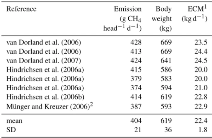
Table 2.Methane emissions calculated with known cow position (GPS) or occupied paddock area (PAD) for different distances of the cow
herd to the EC tower (near, far), and calculated without using cow position information (FIELD). All values, except n, are in units g CH4
head−1d−1.
GPS PAD FIELD
near cows far cows near cows far cows
Mean 423 282 443 319 389a/470b
±2 SE ±24 ±32 ±32 ±40 ±184b
Median 408 296 405 323 348b
SD 168 124 226 173 243b
n 194 63 198 74 7b
aMean of all available 30 min data over the entire grazing period (in contrast to the second
value).
bStatistical values calculated based on monthly results (April–October).
calculated for thenear cowscases were significantly larger than emissions calculated for thefar cowscases. The unctainty of the mean (2 SE, calculated according to Gaussian er-ror propagation) was lowest for the GPS methodnear cows.
Emission results calculated with the PAD method were com-parable to those of the GPS method considering the distance classes. The difference between median and mean values for GPS and PAD method were relatively small indicating sym-metric distribution of individual values. Because the result of the FIELD method was calculated as temporal mean over the entire grazing period (with many small soil fluxes and few large cow influenced fluxes, see Fig. 6), the uncertainty could not be quantified from the variability of the individual 30 min data. Therefore we applied the FIELD method also to monthly periods and estimated the uncertainty (±184 g CH4
head−1d−1) from those results (n
=7). It is much larger than for the two other methods and there is also a considerable dif-ference between the two different mean values.
3.3.2 Diurnal variations
Average diurnal cycle analysis for the near cows cases (Fig. 10a) showed persistent CH4emissions by the cows over
the entire course of the day. For 4 h of the day, less than five values per hour were found, mainly around the two milk-ing periods or durmilk-ing nighttime. Mean emissions per hour ranged from 288 to 560 g CH4head−1d−1with the highest
values in the evening and lowest in the late morning (disre-garding hours withn <5). Although the two grazing periods
(evening/night: 17:00 to 03:00, and morning/noon: 08:00 to 14:00) between the milking phases were not equally long, comparable numbers of values were available (n=91 vs. 103). After the morning milking, the emissions decreased slightly for the first 3 h followed by a slight increase. An al-most opposite pattern could be found after the second milk-ing in the afternoon.
The temporal pattern of cow activity classes (Fig. 10b) mainly followed the daylight cycle with grazing activity dominating during daytime and ruminating during darkness.
Emission [gCH
4
head
−
1 d
−
1]
0
200
600
1000
quartile range median mean 2SE
milking periods
(a)
0
10
20
n
0
10
20
30
40
50
60
Min
utes per hour
00:00 04:00 08:00 12:00 16:00 20:00 00:00
(b)
Figure 10. (a)Average diel variation of CH4cow emissions (GPS
method) for thenear cowscases. White quartile range boxes
indi-cate hours where less than five values are available. The uncertainty is given as 2 SE (black lines). White bars (bottom) show the num-ber of values for each hour (right axis). The two gaps indicate the time when the cows were in the barn for milking. The dashed line in the second milking period indicates that the cows sometimes stayed
longer in the barn.(b)Average time cows spent per hour for grazing
(green), ruminating (yellow), and idling (white) activity, mean diel cycle for the entire grazing season.
Highest grazing time shares were observed right after the milking in the morning and in the later afternoon. While grazing and ruminating show clear opposing patterns, there is no distinct overall relationship with the CH4emission
cy-cle in Fig. 10a. However, maximum emissions in the evening hours coincide with maximum grazing activity.
4 Discussion
4.1 Flux data availability and selection