www.atmos-meas-tech.net/7/3579/2014/ doi:10.5194/amt-7-3579-2014
© Author(s) 2014. CC Attribution 3.0 License.
Measurements of diurnal variations and eddy covariance (EC)
fluxes of glyoxal in the tropical marine boundary layer:
description of the Fast LED-CE-DOAS instrument
S. Coburn1,2, I. Ortega1,2, R. Thalman1,2,*, B. Blomquist3, C. W. Fairall4, and R. Volkamer1,2
1Department of Chemistry and Biochemistry, University of Colorado, Boulder, CO, USA 2CIRES – Cooperative Institute for Research in Environmental Sciences, Boulder, CO, USA 3Department of Oceanography, University of Hawaii, Honolulu, HI, USA
4Earth System Research Laboratory, NOAA, Boulder, CO, USA *now at: Brookhaven National Laboratory, Upton, NY, USA
Correspondence to:R. Volkamer (rainer.volkamer@colorado.edu)
Received: 14 May 2014 – Published in Atmos. Meas. Tech. Discuss.: 20 June 2014
Revised: 10 September 2014 – Accepted: 19 September 2014 – Published: 28 October 2014
Abstract.Here we present first eddy covariance (EC) mea-surements of fluxes of glyoxal, the smallest α-dicarbonyl product of hydrocarbon oxidation, and a precursor for sec-ondary organic aerosol (SOA). The unique physical and chemical properties of glyoxal – i.e., high solubility in water (effective Henry’s law constant, KH=4.2×10⁵M atm−1)
and short atmospheric lifetime (∼2 h at solar noon) – make it a unique indicator species for organic carbon oxidation in the marine atmosphere. Previous reports of elevated glyoxal over oceans remain unexplained by atmospheric models. Here we describe a Fast Light-Emitting Diode Cavity-Enhanced Dif-ferential Optical Absorption Spectroscopy (Fast LED-CE-DOAS) instrument to measure diurnal variations and EC fluxes of glyoxal and inform about its unknown sources. The fast in situ sensor is described, and first results are presented from a cruise deployment over the eastern tropical Pacific Ocean (20◦N to 10◦S; 133 to 85◦W) as part of the Tropi-cal Ocean tRoposphere Exchange of Reactive halogens and Oxygenated VOCs (TORERO) field experiment (January to March 2012). The Fast LED-CE-DOAS is a multispectral sensor that selectively and simultaneously measures glyoxal (CHOCHO), nitrogen dioxide (NO2), oxygen dimers (O4),
and water vapor (H2O) with∼2 Hz time resolution (Nyquist
frequency ∼1 Hz) and a precision of ∼40 pptv Hz−0.5 for glyoxal. The instrument is demonstrated to be a “white-noise” sensor suitable for EC flux measurements. Fluxes of glyoxal are calculated, along with fluxes of NO2, H2O, and
O4, which are used to aid the interpretation of the glyoxal
1 Introduction
Eddy covariance (EC) fluxes are a well-established and widely used technique to measure surface–atmosphere gas exchange. The EC flux method provides insight into sources and sinks of atmospheric parameters (physical and chemical state variables) suitable to test our process-level understand-ing (Baldocchi et al., 2001). EC fluxes are defined as the time average covariance between deviations from the mean of ver-tical wind velocity and deviations from the mean in the pa-rameter of interest, e.g., here, the mixing ratio of a trace gas:
Fc=w′c′= fn Z
0
Cwc(f )df , (1)
whereF is the flux,w′is the vertical wind velocity compo-nent, c′ is the mixing ratio of the trace gas component, the prime denotes the instantaneous deviation from the mean,fn
is the Nyquist frequency of the measurements, andCwcis the
cospectrum.
A requirement of the EC flux technique is that measure-ments of both vertical wind velocities and the trace gas of interest are performed at high sampling frequencies,f (typ-ically a minimum of several Hz), sufficient to capture a ma-jority of those frequencies that contribute to the overall flux. Balancing this requirement with preserving sufficient sen-sitivity in the measurements is one of the major challenges with developing chemical sensors suitable for EC flux appli-cations. For mobile deployments, a portable and robust sen-sor is needed. Further, additional measurements of platform motion need to be performed, and corrections on the wind ve-locity data are needed. A description of the system deployed in this study and the method of correction is described by Fairall et al. (1997) and Edson et al. (1998), respectively. A particular challenge arises for EC flux measurements of short-lived species in the marine boundary layer (MBL), for which concentrations often do not exceed tens to hundreds of parts per trillion (1 pptv=10−12 volume mixing ratio (VMR) =2.46×10⁷molecules cm−3 at 298 K temperature and 1013 mbar pressure). As a result of these challenges, ship based EC flux measurements have today only been reported for the seven trace molecules: dimethyl sulfide (DMS) (Hue-bert et al., 2004; Blomquist et al., 2006, 2010; Marandino et al., 2007, 2008, 2009; Miller et al., 2009; Bell et al., 2013), carbon dioxide (CO2)(Fairall et al., 2000; McGillis et al.,
2001, 2004; Kondo and Tsukamoto, 2007; Miller et al., 2009, 2010; Taddei et al., 2009; Edson et al., 2011; Norman et al., 2012), ozone (O3)(Bariteau et al., 2010; Helmig et al.,
2012), carbon monoxide (CO) (Blomquist et al., 2012), ace-tone (Marandino et al., 2005; Taddei et al., 2009; Yang et al., 2014), acetaldehyde (Yang et al., 2014), and methanol (Yang et al., 2013). Table 1 lists typical concentrations for these molecules in the MBL and compares them with glyoxal in terms of their Henry’s law constants (KH, at 298 K) and
typ-ical atmospheric lifetimes. Notably, glyoxal is the molecule
with the shortest atmospheric lifetime, and it is present in the lowest abundance. The short lifetime of glyoxal limits the spatial scale over which it can be transported in the at-mosphere to a few tens of kilometers. Further, glyoxal is the most soluble molecule in Table 1; i.e., its Henry’s law con-stant is 2000, 13 860, and 30 000 times larger than that of the other oxygenated hydrocarbons (OVOC) methanol, acetone, and acetaldehyde, respectively. The differences in the phys-ical and chemphys-ical properties have fundamental implications for the air–sea exchange of glyoxal. For example, while it is possible to supersaturate the surface ocean with acetaldehyde (Zhou and Mopper, 1990; Kieber et al., 1990; Millet et al., 2010; Yang et al., 2014), it is impossible to supersaturate the ocean with glyoxal (Sinreich et al., 2010). Studies measur-ing the waterside concentration of glyoxal have values in the nanomolar (nM) range (Zhou and Mopper, 1990: 0.5–5 nM; van Pinxteren and Herrmann, 2013):∼4 nM), while based onKH,glyoxal and an airside VMR of 50 pptv the expected
seawater concentration should be∼20000 nM. The low oxal abundance in the MBL and unique properties make gly-oxal a particularly interesting, yet challenging, molecule to measure EC fluxes. To the best of our knowledge there have been no previous attempts to measure EC fluxes of glyoxal.
Table 1.Overview of eddy covariance flux measurements from ships.
Molecule MBL concentration KH Lifetime∗ Reference flux
(pptv) (M atm−1) (days) measurement in MBL
CO2 380–400 (×106) 0.035 >3×10⁵ Fairall et al. (2000)
CO 60–150 (×103) 1×10⁻³ 16 Blomquist et al. (2012) Acetone 700–900 30.3 10 Marandino et al. (2005) O3 10–30 (×103) 0.011 6 Bariteau et al. (2010)
Methanol 300–900 222 4 Yang et al. (2013)
DMS 20–1500 0.485 0.8 Hubert et al. (2004)
Acetaldehyde 200–300 14.1 0.2 Yang et al. (2014) Glyoxal 25–80 4.2×10⁵ 9×10⁻² This work
∗Lifetimes calculated against reaction with OH (assuming [OH]=3×10⁶molecules cm−3), and photolysis rates calculated for aerosol-free, noontime-at-Equator conditions.
Imaging Absorption spectroMeter for Atmospheric CHar-tographY (SCIAMACHY) satellite (Stavrakou et al., 2009). Over the tropical ocean, atmospheric models predict virtu-ally no glyoxal (Myriokefalitakis et al., 2008; Fu et al., 2008; Stavrakou et al., 2009); the presence of this molecule in the remote MBL, thousands of kilometers from continental sources, is surprising and currently not understood (Sinreich et al., 2010).
The University of Colorado Fast Light-Emitting Diode Cavity-Enhanced Differential Optical Absorption Spec-troscopy (Fast LED-CE-DOAS) instrument was developed to obtain new insights about the sources of glyoxal in the re-mote MBL. The following sections describe the instrument, characterize performance, and report first results from a ship deployment over the tropical eastern Pacific Ocean during the Tropical Ocean tRoposphere Exchange of Reactive halogens and Oxygenated VOCs (TORERO) field experiment.
2 Experimental
The TORERO 2012 field campaign was an extensive effort to measure a variety of atmospheric parameters and trace gases over the eastern tropical Pacific Ocean from aircraft and ships. The ship-based portion of the campaign took place aboard the NOAA RV Ka’imimoana on a research cruise leaving from Honolulu, HI, to Puntarenas, Costa Rica, be-tween 25 January and 1 March 2012 (37 days at sea). Fig-ure 1 shows a map with the ship track. Also shown are HYS-PLIT 5-day back trajectories for noon and midnight (local time) along the ship track for each day.
2.1 Fast LED-CE-DOAS instrument
Differential optical absorption spectroscopy (DOAS) is a well-established technique that has been successfully used to measure a wide variety of atmospheric trace gases, including glyoxal (Platt, 1994). While traditionally DOAS measure-ments were conducted in the open atmosphere (Platt et al.,
Figure 1.Cruise track of the NOAA RVKa’imimoanaduring the TORERO 2012 field experiment (red trace). The ship set sail from Honolulu, HI, on 25 January 2012 and made final port in Puntare-nas, Costa Rica, on 1 March 2012 (37 days at sea). Shown along the ship track are HYSPLIT 5-day back trajectories (initiated at 00:00 and 12:00 LT every day; solid grey lines). The black circles along the trajectories are spaced by 1 day. Air sampled in the Northern Hemisphere had been over the ocean for at least 2 days prior to reaching the ship and often did not experience land influences for at least 5 days. Air sampled in the Southern Hemisphere had been over the ocean for more than 5 days without obvious land/pollution influences. The location of the example glyoxal spectrum is marked by the green star.
Figure 2. Example spectra of molecules measured by the Fast LED-CE-DOAS instrument. The DOAS fits are shown for gly-oxal (left panel, 433–460 nm fit window), O4 and NO2 (right
panel, 457–487 nm), and water vapor (both windows). The RMS residual for each fit is shown in the top row. The spectra shown here were recorded on 14 February 2012 at∼06:20 LT (glyoxal) and 11 February 2012 at ∼13:40 LT (O4). The corresponding
slant column density for each trace gas is also given in units of molecules cm−2, except O4, which has units of molecules2cm−5.
In brief, an LED light source is coupled to an optical cavity enclosed by two highly reflective mirrors, which allows light paths inside the cavity to be realized that are much longer (∼2×10⁴ times) than the length of the cavity itself. The light is collected from the backside of the mirror opposite the LED by an optical fiber and directed onto the spectrometer slit (see Fig. 4).
For this system, a high-power LED (LedEngin model number LZ1-00B205; peak optical power 1.3 W) with peak emission near 465 nm was used in conjunction with custom coated mirrors (Advanced Thin Films) with peak reflectivity between 440 and 470 nm. The cavity had a base length of 86 cm (74.45 cm sample path length) and was coupled to a Princeton Instruments Acton SP2156 Czerny–Turner imag-ing spectrometer with a PIXIS 400B CCD (charge-coupled device) detector (1340×400 pixels or 26.8×8 mm). The spectrometer utilized a custom 1000 g mm−1grating blazed at 250 nm which covered the wavelength range of 390– 530 nm with∼0.75 nm resolution (full width at half maxi-mum, or FWHM).
The wavelength range observed simultaneously by our system was from 430 to 480 nm and allowed for the selec-tive detection of glyoxal, NO2, H2O, and O4. Two
spec-tral fitting windows were utilized during this study: one op-timized for the retrieval of glyoxal and the other for O4.
The glyoxal fitting window covered the wavelength range of 433–460 nm; the O4window covered the range 457–487 nm;
and trace gas reference cross sections for glyoxal (Volka-mer et al., 2005), H2O (measured with this instrument), O4
Figure 3.Fast LED-CE-DOAS instrument performance: sensitiv-ity. The residual noise (RMS) from the DOAS analysis is shown as a function of the number of photons corresponding to different averaging of the data. Grey points represent all data, while colored squares represent their respective mean value; black circles repre-sent the theoretical RMS value determined from photon-counting statistics (Coburn et al., 2011). The corresponding 1σ precision of glyoxal is plotted on the right axis.
(Thalman and Volkamer, 2013), and NO2 (Vandaele et al.,
1998) were simultaneously fitted in both windows. Figure 2 shows spectral fit results from the DOAS analysis of these trace gases: the left column shows fits from the glyoxal anal-ysis window for a clean period (no NO2contamination from
the ship stack), and the right column shows spectral fits from the O4window where some NO2 contamination is present.
The water measurement was used to monitor ambient condi-tions, NO2was used as a tracer for sampling the ship stack
plume, and the O4 measurement was used to correct the
DOAS data for sampling time lag and inlet characterization (discussed in Sects. 3.1.1 and 3.1.2).
The primary measurement of the DOAS technique is slant column density (SCD), which is the integrated concentration of the measured species along all light paths. It is easily con-verted using Lambert–Beer’s law to concentration if the light path length within the cavity is known. Two different meth-ods were utilized to experimentally determine the cavity light path: (1) comparison of measured O4SCDs and the
calcu-lated concentration of O4 within the cavity, and (2) using
the ratio of the signal measured in two different pure gases whose Rayleigh scattering cross sections are well known (Thalman and Volkamer, 2010). For this study, method 2 was employed and N2and He were used for this process (referred
an inherent consistency check exists from the comparison of O4SCD measurements with those calculated from the
mir-ror curve, the Rayleigh scattering cross section of air, and known temperature and pressure (Thalman and Volkamer, 2010). For the duration of the cruise, the peak mirror re-flectivity was maintained between 99.9967 and 99.9973 %, translating into routine cavity path lengths of 18–20 km at 455 nm.
In order to accelerate the data acquisition of the instru-ment to rates sufficient to accommodate EC fluxes, soft-ware was developed to simultaneously eliminate shutter movements and decrease readout time (through binning of CCD rows). The final instrument measurement frequency of ∼2 Hz strikes a balance between time resolution and the duty cycle dedicated to collecting photons (as compared to readout time of the CCD). The measurement detection limit with CE-DOAS measurements is typically photon shot-noise-limited. We assess the instrument performance by in-vestigating the root mean square (RMS) of the optical den-sity of the residual remaining after the nonlinear least squares fitting routine and by comparing it with the theoretical pho-ton shot noise (Coburn et al., 2011). Individual spectra were summed and analyzed to improve the signal-to-noise ratio of the measurements. In an ideal instrument (i.e., completely limited by photo shot noise), the RMS of the fitting routine should follow photon-counting statistics, where the theoret-ical RMS is inversely proportional to the square root of the number of photons collected.
RMS≡√1
N, (2)
whereNis the number of photons collected.
The measured RMS of the Fast LED-CE-DOAS instru-ment field deployinstru-ment is compared to the theoretical RMS and plotted as a function of the number of photons in Fig. 3. The grey points are raw data at different levels of averaging, and the colored squares represent the median values for each set: light blue is the raw 400 ms data; dark blue is the sum of 5 spectra (∼2 s); purple is the sum of 20 spectra (∼8 s); red is the sum of 100 spectra (∼40 s); and the green is the sum of 1000 spectra (∼8 min). As can be seen, the RMS during this campaign fairly closely follows counting statistics for the measured spectra, as well as for different levels of binning. Shown on the right axis is the corresponding 1σ precision for glyoxal.
Appropriate quality assurance filters were applied to the raw CE-DOAS measurements prior to calculating glyoxal fluxes in order to exclude the use of any stack contamination, or otherwise questionable data. These filters removed periods of elevated NO2(contaminated by the ship stack plume:
val-ues greater than∼30 pptv), instability in the cavity (O4and
internal cavity pressure measurements: acceptable pressure range 470–500 torr) and any spectra where the DOAS fitting resulted in RMS values larger than 5×10⁻³.
2.2 TORERO field campaign
While the cruise started on 25 January 2012, only data taken during 2 and 28 February 2012 will be considered for this study. The inlet for the cavity was mounted near the top of a 10 m jack staff (18 m above sea level, a.s.l.) on the bow along with the inlets for the CO2flux system (Blomquist et
al., 2014) and the in situ O3 monitor, the sonic
anemome-ter, and a motion system. The sampling line between the inlet and the instrument was∼65 m long and consisted of 3/8 in. inside-diameter coated aluminum tubing (Eaton Syn-Flex Type 1300). Additionally, an aerosol filter (changed ev-ery other day) was included after the inlet in order to pre-vent collection of sea salt in the sampling line and to keep the air reaching the CE-DOAS system aerosol-free. The fil-ter was regularly changed to avoid aerosol accumulation, and experiments of glyoxal transfer through Teflon filters showed no visible attenuation (Thalman and Volkamer, 2010). In order to maintain turbulent flow throughout the sampling line, a high-flow pump maintained a flow of∼120 L min−1
(Lenschow and Raupach, 1991). From this main flow, a sam-ple flow of∼9 L min−1was pulled through the cavity. These
flow conditions resulted in an operating pressure inside the cavity of∼470–500 torr. This sub-ambient cavity pressure had to be actively addressed due to the sensitivity of opti-cal cavities to fluctuations in pressure (which can de-align the mirrors). This was accomplished by the addition of sta-bilizing mounts for the mirrors to prevent movement during measurements. Figure 4 contains a plumbing diagram for the CE-DOAS system, with arrows indicating the direction of air flow at various points along the sampling line. Two pumps and three mass flow controllers (MFCs) were used in this system: the main flow through the sampling line was set at
∼120 L min−1 (controlled by MFC 1), the smaller sample
flow through the cavity was set at∼9 L min−1 (controlled
by MFC 2), and the calibration gases for the Fast LED-CE-DOAS system (used for monitoring cavity performance and determining cavity path length) were controlled by MFC 3. Photographs of the inlet, operational cavity, and instrument rack containing all controlling electronics and spectrometer can be found in Fig. S1 in the Supplement.
3 Results
3.1 Instrument characterization
The following sections will describe the characterization of instrument properties pertinent to the measurement of fluxes via the EC technique.
3.1.1 Phase correction (N2pulse)
Figure 4.Sketch of the Fast LED-CE-DOAS setup and plumbing diagram for sampling during TORERO 2012. The N2“puff” system
is indicated by the red box, and a graphic of the sonic anemometer is shown at the top of the tower. Arrows show the direction of flow through various portions of the system. Photographs of this setup can be found in Fig. S1. The bandpass (BP) and GG 420 filters are used to further narrow the wavelength range of light reaching the spectrometer to that around the peak reflectivity of the mirrors. The lenses utilized in this setup were selected based the incident light and the space allocated for the optics, necessitating the use of both
f/1 andf/4 focal length lenses. MFC: mass flow controller.
degrading the high resolution wind data, the CE-DOAS mea-surements were first interpolated from 2 to 10 Hz. Since the trace gas is drawn through an inlet, there is a finite time dif-ference between the instantaneous wind velocity measure-ments and those of the trace gas measuremeasure-ments. The flux system deployed here includes a method for experimentally determining this correction. The method is described in de-tail in Bariteau et al. (2010), so only a brief overview will be given here: the inlet is equipped with a fast-switching solenoid valve that injects pure nitrogen (supplied from a compressed air cylinder) into the sample flow. The valve is triggered for 3–5 s at the beginning of every hour, and the signal used as the trigger is recorded on the same timestamp as the anemometer. These data are used in conjunction with the accompanied drop in the trace gas signal (recorded on a different timestamp) to continuously monitor and apply a correction to the timestamps prior to correlating both sen-sors. In the cavity, the measurement of O4was used for this
correction. Figure 5 contains a plot showing an example of the corrected O4signal overlaid on the nitrogen pulse signal
(black trace); also shown is the fit of the step response func-tion from method 1 (blue trace; see below). The raw O4
mea-surements are shown as black circles, and the interpolated data are the smaller red circles. Two methods were used to determine the phase correction based on the drop in the O4
signal: (1) fitting of a first-order step response function (2) and manual determination. Method 2 involved using O4data
averages to identify when the N2was attenuating the O4
nal, and from there to determining the time at which the sig-nal actually started dropping. Each asig-nalysis was performed on hourly data files; 626 files were analyzed, and 50 of these files did not meet basic criteria to enable the pulse matching and so were rejected; the total number of usable hours for the
Figure 5.Illustration of the phase correction and time response us-ing O4. Individual CE-DOAS O4measurements (black dots) were
interpolated onto the timestamp of the wind sensor (red dots). The N2pulse signal (solid black line) is visible as the drop in O4SCDs;
the data have already been time-shifted to match this N2 trigger. Also shown is the fit of a step response function (solid blue line) to the drop in the O4signal, from which an instrument time response
can be determined.
Figure 6.Fast LED-CE-DOAS instrument performance: frequency response for glyoxal. The glyoxal variance distribution per fre-quency bin is for a 6 h section of data (representative of the global average) on 4 February 2012 from 06:00 to 12:00 LT. The horizontal line represents the integral variance (∼1600 ppt2Hz−1)at frequen-cies measured by the instrument (green shading). The solid vertical line represents the cutoff frequency determined from the average time response of the instrument; the dashed vertical lines represent the standard deviation of the time response data (grey background shading); higher frequencies were not measured by our setup (red shading). The Nyquist frequency of our setup is 1 Hz.
3.1.2 Response time
The pulse of nitrogen described in the previous section was also used to characterize the response time of the instrument. Introducing pure N2gas into the sample flow created a drop
in the O4 signal, which was exploited to determine the
re-sponse time of the instrument. The same two methods em-ployed for the phase correction were used to calculate the instrument response time, which also gave an average differ-ence between methods of 0.11 s (statistics in Table 2). The instrument response is best determined experimentally, since high-frequency flux attenuations can be caused by drawing the sample through the aerosol filter and long sampling line. Here, a low-pass filter function was chosen to represent the attenuation.
H (f )= 1
1+(2π f τc)2, (3)
whereτcis the instrument response time.
Using the measured response time and the filter function, the instrument cutoff frequency (Fc)(the frequency at which
the signal fluctuations drop by 1/√2)was calculated, which corresponds to a drop in the signal to 0.5.
Fc=
1 2π τc
(4) Using the average values of the response time of 0.283 and 0.282 s for the first-order step response function and the manual determination, respectively, the calculated cutoff fre-quency is 0.56 Hz. The application of the filter function for this system and the effect of the response time on the high-frequency attenuation will be discussed in Sect. 3.3.1. These small differences in response time determined from the two methods add certainty about the correction of the flux mea-surements, as is discussed in more detail in Sect. 3.3.3. 3.1.3 Fast measurements
The variance spectra for glyoxal as a function of frequency for a 6 h time period on 4 February 2012 from 06:00 to 12:00 LT are shown in Fig. 6. Data from both 10 min (purple) and 30 min (light blue) averaging periods (see Sect. 3.3.2) are included in this plot.
The constant variance per Hz in the frequency range sam-pled by the instrument demonstrates that the Fast LED-CE-DOAS system is indeed a white-noise sensor. The horizontal black line represents the integral of the data in the frequency range 6×10⁻⁴ to 1 Hz of
∼1585 pptv2. The solid vertical
black line depicts the cutoff frequency of the instrument cal-culated from the average response time of the instrument, and the dashed vertical black lines represent±1 standard devia-tion of these data.
3.2 Diurnal cycle measurements
Analyzing data created from summing 1000 spectra (∼8 min total integration time) enabled the measurement of a diurnal cycle of glyoxal between 2–28 February 2012. A time series of these measurements can be found in Fig. 7 (top panel, left axis). Summing 1000 spectra allowed the realization of an average RMS value of (1.0±0.1)×10−4, which translates into an average detection limit of 5.9 pptv over 8 min; lower detection limits are possible from further averaging of the data. Figure 3 indicates that the reduction in the achievable 1-σ precision follows the theoretical RMS over several min-utes, and becomes limited by the photon shot noise of the reference spectrum at longer times (rolling-off in the “the-oretical RMS” trace). In the absence of this reference-noise limitation, a photon count over 1 h (3×10⁹photons) corre-sponds to an extrapolated 1-σ precision of 0.8 pptv, and a
3-σ detection limit (1 h) of∼2.4 pptv glyoxal. If, instead, the detection limit is calculated based on averaging the statisti-cal variability of the VMR data, the 3-σ detection limit (1 h) is∼2.2 pptv. This sensitivity is needed to resolve the small changes in the diurnal variation of glyoxal shown in Fig. 7. Also shown are time traces for in situ O3, solar zenith angle
(SZA), NO2, RH, ambient air temperature, ambient pressure,
wind speed (from the sonic anemometer), and a flag indicat-ing periods that were suitable for EC fluxes. Figure S2 con-tains time traces of the parameters used to determine periods that were suitable to perform the EC flux calculations. 3.3 Ambient flux measurements
3.3.1 Signal attenuation
As introduced in Sect. 3.1.2, a low-pass filter function was used to assess the high-frequency flux attenuation due to the aerosol filter and sampling line length; Eq. (1) can be re-written as Eq. (5):
Fc=w′c′m= fn
Z
0
Cwc(f )[H (f )] 1 2df =
fn Z
0
Cwcm(f )df , (5)
where the subscript m represents the measured values; see Eq. (1) for other variables (note that the square root appears in the modified equation because only the signal of the trace gas is attenuated).
This relationship can then be used to assess the effect of attenuation on the overall flux by applying the filter func-tion using the Kaimal model neutral-stability cospectrum (Kaimal et al., 1972), derived via Eqs. (6a) and (6b):
f Cwc(f )
Fc =
11n
(1+13.3n)1.75, n≤1.0 (6a) f Cwc(f )
Fc =
4.4n
Table 2.The average phase correction and time response of the Fast LED-CE-DOAS instrument (with standard deviation) for the two different methods employed in this study. See text for details.
Method 1 Method 2
Phase Time Phase Time
correction (s) response (s) correction (s) response (s)
Average −2.54 0.28 −2.61 0.28
Standard deviation 0.23 0.16 0.24 0.14
Figure 7.Time series of glyoxal, O3, and NO2, as well as meteorological parameters. Grey shaded background represents times suitable for
flux calculations; filters included NO2, cavity pressure, wind direction, wind direction standard deviation, ship heading range, dGly/dt, and
the horizontal glyoxal flux components. See text and Fig. S2 for details.
where the surface normalized frequencyn=f z/ur,zis the
measurement height, and ur is the average relative wind
speed. Using the calculated “true” and “measured” Kaimail cospectra, an attenuation ratio (Rattn)was derived.
Rattn(z, ur)= fn R
0
Cwc_K(f, z, ur)[H (f )] 1 2df fn
R
0
Cwc_K(f, z, ur)df
=
fn R
0
Cwcm_K(f, z, ur)df fn
R
0
Cwc_K(f, z, ur)df
=
fn R
0
Cwcm(f, z, ur)df fn
R
0
Cwc(f, z, ur)df
=Fxm
Fx
, (7)
whereCwc_Kdenotes the Kaimal cospectrum. For the
calcu-lation of this ratio, the average value of 0.282 s for the instru-ment response time was used in the filter response function
H (f ). The assessment of these data leads to an average at-tenuation ratio of 0.947 but never resulted in more than a 10 % correction.
3.3.2 Flux filtering and results
Figure 8. Cospectra of glyoxal and vertical wind from the flux calculations. The green trace represents the average of all tra that passed the quality assurance filters. The positive cospec-trum (red) represents data averaged over a period of∼3.5 h from 21:15 LT on 16 February 2012 to 00:45 LT on 17 February 2012. The negative cospectrum (blue) represents a ∼1 h average on 2 February 2012 from 14:45 to 15:45 LT. The background color shading is identical to that in Fig. 6.
filtering criteria were applied to exclude outliers in the flux data through the assessment of the horizontal components of the glyoxal flux and the rate of change of glyoxal for each data segment. These filter values were chosen rather arbi-trarily through a visual inspection of the data. No significant differences were found between the four data sets. Only re-sults from the 30 min data determined from phase correction method 2 will be discussed. While individual flux measure-ments proved to be noisy, further binning of the 30 min flux measurements reveals trends in the data. Figure 8 contains example cospectra from these data, where the average of all data (green trace) scatters around zero. The examples of both positive (red trace) and negative (blue trace) cospectra were created by binning data: from 21:15 LT on 16 February to 00:45 LT on 17 February (positive cospectrum); and from 14:45 to 15:45 LT on 2 February (negative cospectrum). 3.3.3 Error sources
The potential sources of error in these data are (1) inaccura-cies in determining the phase shift of the CE-DOAS measure-ments, (2) high-frequency signal loss due to sampling line at-tenuation, and (3) uncertainty surrounding the noisy raw gly-oxal measurements. Phase shift determination was deemed to be rather robust (through the comparison of the values de-termined using the two different methods), and any small inaccuracies would have negligible effect on the flux data (as assessed by comparing the results from the four meth-ods previously mentioned). The high-frequency flux loss due
to signal attenuation was calculated as being, at most, 10 % from the characterization in the instrument response time. Based on the cospectra (Fig. 8), it seems that glyoxal effi-ciently transferred through the sample lines and using the O4 measurements to characterize sample transfer is a
justi-fiable assumption. Additionally, in the DOAS analysis there exists potential for cross correlations between water and gly-oxal due to overlapping absorption features; however the most prominent absorption features are shifted and thus well separated (water:∼443 nm; glyoxal:∼455 nm). The effect of water on glyoxal retrievals was assessed in Thalman et al. (2014), where a very similar cavity-enhanced DOAS in-strument was compared with numerous other techniques to measure alpha-dicarbonyls. The glyoxal retrieval is rela-tively insensitive to the presence of water. However, in order to rule out any effect of cross correlations in the glyoxal flux measurements, the eddy covariance flux method was applied to our water absorption data and water fluxes were derived in the same manner as that for the glyoxal measurements. Fig-ure S3 contains correlation plots of glyoxal and water flux measurements, which show no distinct trends and indicate that the retrieval of glyoxal fluxes in this study is indeed in-sensitive to water absorption. While the glyoxal flux changes direction depending on time of day, the water flux is always positive, reflecting evaporation (see Sect. 4.2.2 and Fig. 10).
4 Discussion
4.1 Volume mixing ratio measurements
Volume mixing ratio data show a persistent diurnal trend: glyoxal mixing ratios peak just before dawn (1 h average maximum in the NH: 43±2 pptv; minimum: 26±1 pptv; maximum SH: 61±1 pptv; minimum: 39±2 pptv), decrease during the day, and reach a minimum in the late evening just after dark (1 h average maximum in the NH: 36±1 pptv; minimum: 16±1 pptv; maximum SH: 48±2 pptv; mini-mum: 24±1 pptv), followed by continuous increase through the night. The day-to-day variability in glyoxal is signifi-cantly larger than the accuracy of our instrument. Major ad-vantages with the Fast LED-CE-DOAS instrument to per-form precise and accurate measurements of glyoxal are its inherent calibration from observing O4(see above) as well
Figure 9.Diurnal variation in the glyoxal(a)and O3mixing ratio (b) in the Northern (blue) and Southern Hemisphere (red). Only data that qualify for flux calculations have been averaged. Yellow shading indicates daytime, while grey indicates nighttime; the SZA is also shown on the right axis.
than that indicated by error bars, which are dominated (e.g., Fig. 9a) by the multiday variability in glyoxal over oceans. Indeed, the error bars for multiday averaged data reflect this variability (standard deviation), rather than the instrument precision/accuracy. Despite this significant day-to-day vari-ability, some trends can be seen if data are segregated as a function of time of day (local time) and geographical loca-tion. Figure 9 shows the glyoxal VMR (panel a) and O3VMR
(panel b) binned as a function of time of day. The data were further segregated for measurements collected in the North-ern Hemisphere (blue, 13◦N to 0) and Southern Hemisphere (red, 0 to 10◦S); the global average of all data is shown as the grey trace. The number of data points within each bin is given in Table 3. The shaded regions in the background indi-cate daytime (yellow) and nighttime (grey), and the average SZA (minimum indicates solar noon) is further shown for reference on the right axis.
Given the nighttime increase in the glyoxal concentration that we observe in both hemispheres, O3 is the most likely
oxidant of the glyoxal precursor. Interestingly, we observe about twice-higher O3concentrations in the NH (∼20 ppbv
O3)than in the SH (∼10 ppbv O3). O3 does not reveal a
significant diurnal cycle in either hemisphere, and the global campaign average O3VMR is∼15 ppbv.
4.2 Eddy covariance flux measurements 4.2.1 Glyoxal
The diurnal variations in our glyoxal flux measurements (Fig. 10a) qualitatively reflect the variations in the VMRs seen in Fig. 9a. The error bars in Fig. 10 reflect the 90 % confidence intervals of data within each bin. The maximum
Figure 10.Diurnal variations in the fluxes of glyoxal(a), NO2(b),
and H2O(c). Data are separated between hemispheres, and the for-mat here is the same as in Fig. 9.
fluxes are seen at night (SH: (5.3±3.3)×10−2pptv m s−1; NH: (2.3±3.1)×10−2pptv m s−1) and minimum fluxes during the daytime (SH: (−1.6±3.8)×10−2pptv m s−1; NH: (−5.6±4.1)×10−2pptv m s−1). All nighttime fluxes in the SH are significantly greater than zero (SH night-time average: (4.7±1.8)×10−2pptv m s−1). The nighttime source of glyoxal from the ocean to the atmosphere is sur-prising, since glyoxal is so water soluble. Previous observa-tions of positive fluxes of less-soluble OVOCs, such as ac-etaldehyde, have been attributed to supersaturation of sub-surface waters in acetaldehyde (Zhou and Mopper, 1990; Yang et al., 2014). Glyoxal formation in subsurface waters cannot explain a positive flux to the atmosphere. This is because of the very large effective Henry’s law coefficient (KH=4.2×10⁵M atm−1), which causes the equilibrium of
glyoxal to be strongly shifted (107:1) towards the ocean (Volkamer et al., 2009). The high KH value of glyoxal is
the result of rapid hydration reactions; once hydrated, gly-oxal exists primarily in mono- and di-hydrated forms (Ruiz-Montoya and Rodriguez-Mellado, 1994, 1995) that give rise to the 3–5 orders of magnitude higherKH value of glyoxal
compared to other OVOCs (see Table 1). Ervens and Volka-mer (2010) estimated the hydration rate of glyoxal to be 7 s−1. This corresponds to a lifetime of glyoxal with respect to hydrolysis of∼140 ms. Unless glyoxal escapes from the ocean within this time frame, it will hydrate and is trapped in hydrated forms in the condensed phase. Using Eq. (8)
D=l
2
2t, (8)
where D is the diffusion coefficient (assuming a range (0.001–1)×10−5cm2s−1; Finlayson-Pitts and Pitts, 2000),
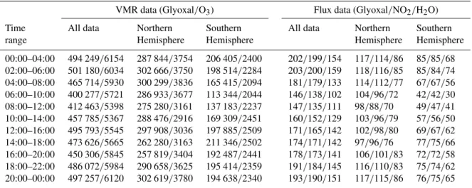
Table 3.Number of points in each time bin from Figs. 9 and 10.
VMR data (Glyoxal/O3) Flux data (Glyoxal/NO2/H2O)
Time All data Northern Southern All data Northern Southern
range Hemisphere Hemisphere Hemisphere Hemisphere
00:00–04:00 494 249/6154 287 844/3754 206 405/2400 202/199/154 117/114/86 85/85/68 02:00–06:00 501 180/6034 302 666/3750 198 514/2284 203/200/159 118/116/85 85/84/74 04:00–08:00 465 714/5930 300 299/3836 165 415/2094 181/179/133 114/112/77 67/67/56 06:00–10:00 400 277/5721 286 933/3677 113 344/2044 146/138/102 104/96/72 42/42/30 08:00–12:00 412 463/5398 275 280/3161 137 183/2237 147/135/111 98/88/70 49/47/41 10:00–14:00 457 785/5367 288 476/2916 169 309/2451 160/152/129 103/96/79 57/56/50 12:00–16:00 495 793/5545 297 908/3036 197 885/2509 171/165/142 102/98/80 69/67/62 14:00–18:00 473 626/5665 262 280/3163 211 346/2502 174/171/142 97/96/76 77/75/66 16:00–20:00 450 306/5845 257 819/3404 192 487/2441 178/173/141 106/101/83 72/72/58 18:00–22:00 486 072/5984 290 658/3625 195 414/2359 191/184/145 116/110/83 75/74/62 20:00–00:00 497 257/6120 302 619/3780 194 638/2340 193/190/151 117/115/86 76/75/65
of only∼0.5–17 µm. Such a short distance rules out glyoxal production in sub-surface waters as a source for the positive glyoxal flux.
It is further unlikely that the observed nighttime posi-tive flux could be attributed to gas-phase chemistry occur-ring below the measurement height but above the ocean sur-face. This is because we generally observe higher glyoxal fluxes and glyoxal VMRs in the SH, where O3 is lower
than in the NH. The gradient in O3between the two
hemi-spheres is the reverse of that in glyoxal VMR. In princi-ple, different precursors and mechanisms could form gly-oxal in the two hemispheres. More likely, we interpret the reversed chemical gradients between both hemispheres to re-flect the fact that the ocean is a net sink for O3 (Helmig
et al., 2012); glyoxal is a product of the chemistry that de-stroys O3at the ocean surface. Faster O3 destruction at the
ocean surface in the SH (reflected in the lower observed O3
VMR) is thus compatible with the positive glyoxal fluxes, and higher glyoxal VMR, that we observe in the SH. As-suming a rather fast (upper limit) reaction rate constant for O3 to react with a glyoxal precursor in the gas phase
(kO3∼10−
15cm3molecules−1s−1; Atkinson et al., 2006),
the corresponding precursor lifetime with respect to O3
re-action is about 45 min (assuming an average O3 VMR of
15 ppbv). Given that the glyoxal concentration increases through much of the night in both hemispheres (Fig. 9), the precursor that forms glyoxal at night is most likely longer lived (possibly a lifetime of several hours). Hence, any gas-phase chemistry below our inlet is unlikely to be sufficiently fast to contribute much glyoxal over the 18 m distance from our inlet to the ocean surface. Furthermore, gas-phase chem-istry below our inlet would produce glyoxal at a twice-higher rate in the NH compared to the SH, while we see lower-glyoxal VMR in the NH and observe positive fluxes primar-ily in the SH. This evidence supports the assignment that the positive glyoxal fluxes observed at night locate a
gly-oxal source inside the organic sea surface microlayer (SML). Chemistry within the SML is likely also a source of other OVOCs (e.g., formaldehyde, aliphatic and multifunctional aldehydes, methylglyoxal, etc.; Zhou and Mopper, 1990; Ay-ers et al., 1997; Zhou and Mopper, 1997; Zhou et al., 2014).
The maximum average positive (net) flux that we observe in the SH at night (5.3×10⁻²pptv m s−1) corresponds to
a primary glyoxal accumulation in a 800 m high MBL of about∼2.5 pptv over a period of 12 h. This corresponds to
∼20 % of the increase in the VMR of glyoxal that is actu-ally being observed over the course of the night. We note that the EC technique measures a net flux, i.e., only the difference between deposition and emission fluxes. Based on the variability in the net flux, it appears that both pro-cesses are contributing to the signal. Given the rapid hy-dration reaction and high solubility of glyoxal, the frac-tion of the glyoxal molecules which deposit to the surface and are later re-emitted is likely small. We can assume that the deposition is essentially a 100 % efficient sink and the emission we see is due to instantaneous production/emission within the SML that compensates for, and exceeds, the deposition flux. The actual surface production flux is the net flux corrected for the deposition flux. The daytime ob-served fluxes are significantly negative (NH daytime average: (−4.6±2.3)×10−2pptv m s−1). Assuming a dry deposition
velocity,vdep=1×10⁻³m s−1, and using the campaign
the balance between production and deposition fluxes, which are likely operative and significant at night. The observed positive (net) fluxes cannot explain the observed increase in the glyoxal VMR at night by the SML source alone.
During the day the observed glyoxal flux is negative and indicates some unknown gas-phase source of glyoxal and likely other OVOCs in the MBL. While negative or neutral fluxes have also been observed for acetone and methanol (Marandino et al., 2005; Yang et al., 2013, 2014), both of these molecules live sufficiently long (acetone: 15 days; methanol: 13 days) for transport from the free troposphere (entrainment fluxes) and from terrestrial sources to likely contribute to their abundance in the remote MBL. By con-trast, any glyoxal lost to the ocean has been produced lo-cally. The daytime lifetime of glyoxal (∼2 h) is too short to explain this source in terms of transport from terrestrial sources. The lack of measurements of glyoxal vertical distri-butions over oceans in the literature complicates discussions of possible entrainment fluxes of glyoxal from the free tropo-sphere. However, for purposes of this discussion any entrain-ment flux could help explain the negative net flux observed during the day, but cannot explain the positive net flux ob-served at night. We conclude that the SML is a significant source of glyoxal. However, the negative daytime net flux in-dicates deposition exceeds SML production during the day. A glyoxal source in the atmosphere is thus needed to sus-tain the elevated glyoxal VMR during the day, and currently remains unexplained. SML production alone appears insuf-ficient to explain the glyoxal abundance and variation inside the MBL.
4.2.2 NO2, H2O, and O4fluxes
Absorption measurements of NO2, H2O, and O4by the Fast
LED-CE-DOAS instrument are a by-product of processing the glyoxal data. The fluxes for these quantities were pro-cessed in the same fashion as the glyoxal fluxes, and diurnal profiles of NO2 and H2O fluxes are shown in Fig. 10. For
NO2, the fluxes are smaller 0.05 pptv NO2m s−1, and no
ev-idence for a NO2 flux diurnal cycle is observed (Fig. 10b).
This is consistent with the idea that NO2is not directly
emit-ted from oceans (Logan, 1983). The median global average of all NO2 flux measurements is −0.04 pptv m s−1. It has
been shown that nitrogen oxide (NO) is photo-chemically produced by the ocean (Zafiriou et al., 1980; Zafiriou and McFarland, 1981; Olasehinde et al., 2010). NO2 is
subse-quently produced from the gas-phase reaction of NO with O3
(kNO,O3=1.8×10−
14cm3molecules−1s−1; Atkinson et al.,
1997). At 15 ppbv O3, this reaction converts NO into NO2on
a timescale of∼2–3 min. The absence of positive NO2fluxes
and lack of a NO2diurnal cycle is compatible with, and
fur-ther corroborates, the indication by positive glyoxal fluxes of chemistry within the SML rather than a gas-phase reaction below our inlet.
The H2O fluxes (Fig. 10c) are on the order of 0.5–
1.5×10⁻³% VMR m s−1 and consistently positive. A
dis-tinct diurnal variation is observed consistently between the NH and SH, with minima just before sunrise and maxima several hours after solar noon. This increase in the H2O
flux indicates faster evaporation of H2O from the ocean
dur-ing the day. Notably, if imperfections in our current knowl-edge about absorption cross sections of water vapor were to severely overlap (and create cross-correlations) with gly-oxal absorption structures, the water fluxes could become a driver for the glyoxal fluxes. However, no evidence for such a cross-correlation is observed. Indeed, while the direction of the water flux is consistently positive, glyoxal fluxes change direction over the course of the day. There is further an offset in the timing of minima/maxima. The independent behav-ior of diurnal variations in the H2O and glyoxal fluxes thus
indicates that both gases are robust, and indicates that miss-ing H2O absorption structures in spectral databases such as
HIgh-resolution TRANsmission (HITRAN) are unlikely to affect the measured glyoxal fluxes.
O4 is not a stable molecule but the result of
collision-induced absorption of two O2 molecules (Thalman and
Volkamer, 2013). If the O4flux is converted to units of
vari-ations in the O2 mixing ratio, the corresponding O2 flux is
always smaller than 10−3% O2 VMR m s−1, which
corre-sponds to concentration changes in O2that are 4–5 orders of
magnitude smaller than the ambient O2VMR of∼20.95 %
(<10 ppm1O2). Fluxes of this magnitude are observed both
positive and negative yet are about 2 orders of magnitude larger than the corresponding fluxes of CO2(Blomquist et al.,
2014). As such, we interpret the O4fluxes to essentially
re-flect the noise in our measurements. These small upper limit fluxes reflect a very stable signal for O4; the change in this
internal calibration gas is smaller: 0.4 % of the typical O4
signal per hour (and not systematic).
Figure S4 shows a selection of ocean and atmospheric state parameters that are binned in the same fashion as the VMR and flux data and separated between NH and SH for archival. 4.3 Context with satellite observations
function of longitude. The average glyoxal VMR in the west-erly NH cruise segment is 32±5 pptv (average over 7 days; 13◦N to 0 latitude; 133 to 105◦W longitude), compared to 31±8 pptv in the easterly NH cruise segment (average over 7 days; 13◦N to 0 latitude; 105 to 80◦W longitude). Early re-ports from SCIAMACHY found the annually averaged (year 2005) VCD of 4.5×10¹⁴ and 6.0×10¹⁴molecules cm−2 VCD over the western and eastern cruise segments in the NH – and 3.5×10¹⁴molecules cm−2over the SH cruise segment (Wittrock et al., 2006). Interestingly, measurements from the Global Ozone Monitoring Experiment-2 (GOME-2) satellite (Lerot et al., 2010) report∼4.5×14molecules cm−2in both regions of the NH, i.e., find no evidence for a longitudi-nal variation in multiyear averaged data (2007 to 2009) and
∼3×10¹⁴molecules cm−2over the SH cruise segment. The
absence of a gradient over 3000 km distance in GOME-2 data is consistent with our data. However, it is interesting to note that the lower-limit VCDs of both satellite instruments cor-respond to∼183 pptv glyoxal in the NH and∼120 pptv gly-oxal in the SH (assuming all glygly-oxal is located inside a 1km high MBL). Such high glyoxal is not confirmed by our ob-servations, or by the measurements of Sinreich et al. (2010). We note that the maximum concentration of 140 pptv re-ported by Sinreich et al. (2010) presents an extremely rare scenario that is not deemed representative of this data set (see their Fig. 3c). In situ and ship MAX-DOAS column ob-servations (Sinreich et al., 2010; Mahajan et al., 2014) agree that there is insufficient glyoxal inside the MBL to explain satellite VCDs; this is particularly true over the NH tropical eastern Pacific Ocean (by a factor 2 to 6). Furthermore, our in situ data show glyoxal is more abundant in the SH tropi-cal MBL. By contrast, both satellites find∼25–42 % lower-glyoxal VCDs in the SH compared to the NH. The campaign average VMR during mornings in the SH (47±7 pptv gly-oxal) corresponds to ∼1.2×10¹⁴molecules cm−2 glyoxal VCD over the SH cruise segment, which is 2–3 times lower than long-time average VCD observed from space. The rea-son for this apparent mismatch in glyoxal amounts, and re-versed hemispheric gradients, is currently not understood. A particularly interesting development to investigate the diur-nal variation of glyoxal over oceans consists in the Tropo-spheric Emissions: Monitoring of Pollution (TEMPO) satel-lite mission (planned to launch in 2019), which will provide first time-resolved glyoxal VCD observations from geosta-tionary orbit. Our diurnal profiles show further that glyoxal concentrations change by 30 % over the course of the day. With the caveat that changes in MBL VMRs may not be in-dicative of VCD changes, this also implies that∼15 % lower VCDs are expected at the time of the Ozone Monitoring In-strument (OMI) satellite overpass (13:45 LT at the Equator). The differences between satellite and in situ measurements are as of yet difficult to reconcile. Notably, a direct compar-ison between in situ observations and column data is com-plicated due to the lack of vertical profile measurements of glyoxal at tropical latitudes, different averaging times, and
spatial scales probed by in situ and column observations, as well as uncertain assumptions about a priori profiles, cloud screening, and other factors that influence air mass factor calculations. Some of these factors were further investigated from collocated measurements of glyoxal from aircraft dur-ing the TORERO project. The fast in situ LED-CE-DOAS instrument holds great potential for future deployments on research aircraft.
5 Conclusions
We have performed the first in situ measurements of glyoxal VMRs over oceans and presented first EC flux measurements of this soluble and short-lived molecule. Data from the first field deployment of the instrument are presented (26 days of measurements). The Fast LED-CE-DOAS instrument is a multispectral sensor suitable to measure eddy covariance fluxes of glyoxal and other gases selectively in the remote MBL. The measurement frequency of ∼2 Hz is sufficient to capture ∼90 % of the glyoxal flux. Inlet and sampling line attenuation was determined using the measured response time of the instrument (0.28±0.14 s, based on O4
measure-ments) and accounts for a correction of <10 %. Multiple other gases are detected simultaneously with glyoxal and are exploited as follows: NO2measurements are used to identify
and filter data affected by stack contamination from the ship, and NO2 fluxes inform discussions about gas-phase
chem-istry below our inlet to be unlikely; H2O measurements are
used to calculate ambient relative humidity, and H2O fluxes
(consistently indicate evaporation) are used for correlative analysis of glyoxal fluxes and reveal a lack of any apparent correlation. Glyoxal is well separated from H2O. The H2O
fluxes help address concerns about spectral cross-correlation between missing water lines in the HITRAN database, and the lack of a H2O and glyoxal correlation further confirms
the robustness of our retrievals. O4measurements in ambient
air are used an internal calibration gas to assure control over cavity alignment and mirror cleanliness (Thalman and Volka-mer, 2010); further the pulsing of nitrogen gas into the inlet is monitored from fast high signal-to-noise measurements of O4 as part of individual spectra. O4 is then used to
charac-terize sample transfer time through the sampling line, and to synchronize the clocks of the chemical sensor with that of the wind sensor. Two different methods showed excellent control over the phase correction from O4measurements
(av-erage difference∼0.11±0.10 s) and give confidence in the EC flux measurements of glyoxal.
over the remote eastern tropical Pacific Ocean, which is in marginal agreement with the campaign average VMR of our in situ measurements. Recent reports of an average
∼25 pptv glyoxal, and no more than 40 pptv, over a wide ar-ray of ocean environments (Mahajan et al., 2014) are slightly lower than our in situ observations. The comprehensive ev-idence generally supports the global presence of glyoxal over oceans as indicated by satellites (Wittrock et al., 2006; Lerot et al., 2010). Global glyoxal observations currently re-main unexplained by atmospheric models (Myriofekalitakis et al., 2008; Fu et al., 2008; Stavrakou et al., 2009), and re-trievals remain uncertain (Lerot et al., 2010; Alvarado et al., 2014; Miller et al., 2014) and largely untested.
The widespread positive flux that we observe in both hemi-spheres at night (more prevalent in the SH) provides direct evidence that the SML is widespread (Wurl et al., 2011), and that oxidation reactions inside the SML are a source for OVOCs. A consistent increase is observed in the glyoxal VMR at night (both hemispheres) and suggests this SML source involves dark reactions of O3 that produce glyoxal.
Notably, a recent laboratory study observed the volatilization of several OVOCs (including glyoxal) when O3was flowed
above a polyunsaturated fatty acid film on artificial saltwa-ter in a flow reactor (Zhou et al., 2014). These results pro-vide qualitative confirmation that the oxidation of the SML by O3can be a source for OVOCs to the gas phase. However,
the production rates found in this laboratory study are in-sufficient to explain any appreciable portion of the observed glyoxal over the tropical Pacific Ocean. The observed net fluxes are the balance between production and deposition fluxes. Observations of positive fluxes of glyoxal indicate that the SML production is significant and can dominate over considerable glyoxal deposition fluxes. Even the extremes among the positive EC net fluxes that we observe (SH at night) can only explain a minor share of the sustained in-crease in glyoxal VMR overnight. The negative net flux dur-ing the day suggests that SML production chemistry is not the only source of glyoxal over oceans, and it points to the need for an atmospheric source to sustain the atmospheric glyoxal VMR during the day. Our observations locate chem-istry at interfaces and emphasize the need to better under-stand heterogeneous chemistry. Heterogeneous chemistry as a source for volatile OVOCs could also be occurring on ma-rine aerosols.
The Supplement related to this article is available online at doi:10.5194/amt-7-3579-2014-supplement.
Acknowledgements. The development of the Fast LED-CE-DOAS sensor was supported by the US National Science Foundation under NSF-CAREER award ATM-847793. The TORERO project is a US-SOLAS contribution, and it is supported by NSF under award AGS-l104104 (PI: R. Volkamer). S. Coburn is a recipient of a NASA Earth and Space Science Fellowship. The authors thank the captain and crew of the RVKa’imimoana, Brian Lake and the NOAA TAO program, and David Welsh for their valuable support during the “TORERO cruise” KA-12-01. Mingxi Yang provided valuable comments on the manuscript.
Edited by: E. C. Apel
References
Alvarado, L. M. A., Richter, A., Vrekoussis, M., Wittrock, F., Hilboll, A., Schreier, S. F., and Burrows, J. P.: An improved gly-oxal retrieval from OMI measurements, Atmos. Meas. Tech. Dis-cuss., 7, 5559–5599, doi:10.5194/amtd-7-5559-2014, 2014. Atkinson, R., Baulch, D. L., Cox, R. A., Hampson Jr., R. F., Kerr,
J. A., Rossi, M. J., and Troe, J.: Evaluated Kinetic, Photochem-ical and Heterogeneous Data for Atmospheric Chemistry: Sup-plement V. IUPAC Subcommittee on Gas Kinetic Data Evalua-tion for Atmospheric Chemistry, J. Phys. Chem. Ref. Data, 26, 521–1011, doi:10.1063/1.556011, 1997.
Atkinson, R., Baulch, D. L., Cox, R. A., Crowley, J. N., Hamp-son, R. F., Hynes, R. G., Jenkin, M. E., Rossi, M. J., Troe, J., and IUPAC Subcommittee: Evaluated kinetic and photochemi-cal data for atmospheric chemistry: Volume II – gas phase re-actions of organic species, Atmos. Chem. Phys., 6, 3625–4055, doi:10.5194/acp-6-3625-2006, 2006.
Ayers, G. P., Gillet, R. W., Granek, H., deServes, C., and Cox., R. A.: Formaldehyde production in clean marine air, Geophys. Res. Lett., 24, 401–404, doi:10.1029/97GL00123, 1997.
Baldocchi, D., Falge, E., Gu, L., Olson, R., Hollinger, D., Running, S., Anthoni, P., Bernhofer, C., Davis, K., Evans, R., Fuentes, J., Goldstein, A., Katul, G., Law, B., Lee, X., Malhi, Y., Meyers, T., Munger, W., Oechel, W., U, K., Pi-legaard, K., Schmid, H., Valentini, R., Verma, S., Vesala, T., Wilson, K., and Wofsy, S.: FLUXNET: A new tool to study the temporal and spatial variability of ecosystem-scale carbon dioxide, water vapor, and energy flux densities, Bull. Am. Meteorol. Soc., 82, 2415–2434, doi:10.1175/1520-0477(2001)082<2415:FANTTS>2.3.CO;2, 2001.
Bariteau, L., Helmig, D., Fairall, C. W., Hare, J. E., Hueber, J., and Lang, E. K.: Determination of oceanic ozone deposition by ship-borne eddy covariance flux measurements, Atmos. Meas. Tech., 3, 441–455, doi:10.5194/amt-3-441-2010, 2010.
Bell, T. G., De Bruyn, W., Miller, S. D., Ward, B., Christensen, K. H., and Saltzman, E. S.: Air-sea dimethylsulfide (DMS) gas transfer in the North Atlantic: evidence for limited interfacial gas exchange at high wind speed, Atmos. Chem. Phys., 13, 11073– 11087, doi:10.5194/acp-13-11073-2013, 2013.
Blomquist, B. W., Huebert, B. J., Fairall, C. W., and Faloona, I. C.: Determining the sea-air flux of dimethylsulfide by eddy cor-relation using mass spectrometry, Atmos. Meas. Tech., 3, 1–20, doi:10.5194/amt-3-1-2010, 2010.
Blomquist, B. W., Fairall, C. W., Huebert, B. J., and Wilson, S. T.: Direct measurement of the oceanic carbon monoxide flux by eddy correlation, Atmos. Meas. Tech., 5, 3069–3075, doi:10.5194/amt-5-3069-2012, 2012.
Blomquist, B. W., Huebert, B. J., Fairall, C. W., Bariteau, L., Edson, J. B., Hare, J. E., and McGillis, W. R.: Advances in Air-Sea CO2 Flux Measurement by Eddy Correlation, Bound.-Lay. Meteorol., 152, 3, 245–276, doi:10.1007/s10546-014-9926-2, 2014. Coburn, S., Dix, B., Sinreich, R., and Volkamer, R.: The CU
ground MAX-DOAS instrument: characterization of RMS noise limitations and first measurements near Pensacola, FL of BrO, IO, and CHOCHO, Atmos. Meas. Tech., 4, 2421–2439, doi:10.5194/amt-4-2421-2011, 2011.
Edson, J. B., Hinton, A. A., Prada, K. E., Hare, J. E., and Fairall, C. W.: Direct covariance flux estimates from mobile platforms at sea, J. Atmos. Ocean. Technol., 15, 547–562, doi:10.1175/1520-0426(1998)015<0547:DCFEFM>2.0.CO;2, 1998.
Edson, J. B., Fairall, C. W., Bariteau, L., Zappa, C. J., Cifuentes-Lorenzen, A., McGillis, W. R., Pezoa, S., Hare, J. E., and Helmig, D.: Direct covariance measurement of CO2gas transfer
veloc-ity during the 2008 Southern Ocean Gas Exchange Experiment: Wind speed dependency, J. Geophys. Res.-Ocean., 116, C00F10, doi:10.1029/2011JC007022, 2011.
Ervens, B. and Volkamer, R.: Glyoxal processing by aerosol multi-phase chemistry: towards a kinetic modeling framework of sec-ondary organic aerosol formation in aqueous particles, Atmos. Chem. Phys., 10, 8219–8244, doi:10.5194/acp-10-8219-2010, 2010.
Fairall, C. W., White, A. B., Edson, J. B., and Hare, J. E.: Inte-grated shipboard measurements of the marine boundary layer, J. Atmos. Ocean. Technol., 14, 338–359, doi:10.1175/1520-0426(1997)014<0338:ISMOTM>2.0.CO;2, 1997.
Fairall, C. W., Hare, J. E., Edson, J. B., and McGillis, W. R.: Parameterization and Micrometeorological Measurement of Air–Sea Gas Transfer, Bound.-Lay. Metorol., 96, 63–106, doi:10.1023/A:1002662826020, 2000.
Finlayson-Pitts, B. and Pitts, J. N.: Chemistry of the upper and lower atmosphere: theory, experiments, and applications, Aca-demic Press, United States of America, 2000.
Fu, T., Jacob, D. J., Wittrock, F., Burrows, J. P., Vrekoussis, M., and Henze, D. K.: Global budgets of atmospheric gly-oxal and methylglygly-oxal, and implications for formation of sec-ondary organic aerosols, J. Geophys. Res.-Atmos., 113, D15303, doi:10.1029/2007JD009505, 2008.
Grosjean, D., Grosjean, E., and Gertler, A. W.: On-road emissions of carbonyls from light-duty and heavy-duty vehicles, Environ. Sci. Technol., 35, 45–53, doi:10.1021/es001326a, 2001. Hays, M. D., Geron, C. D., Linna, K. J., and Smith, N. D.:
Spe-ciation of Gas-Phase and Fine Particle Emissions from Burn-ing of Foliar Fuels, Environ. Sci. Technol., 36, 2281–2295, doi:10.1021/es0111683, 2002.
Helmig, D., Lang, E. K., Bariteau, L., Boylan, P., Fairall, C. W., Ganzeveld, L., Hare, J. E., Hueber, J., and Pal-landt, M.: Atmosphere-ocean ozone fluxes during the TexAQS 2006, STRATUS 2006, GOMECC 2007, GasEx 2008, and
AMMA 2008 cruises, J. Geophys. Res.-Atmos., 117, D04305, doi:10.1029/2011JD015955, 2012.
Huebert, B., Blomquist, B., Hare, J., Fairall, C., Johnson, J., and Bates, T.: Measurement of the sea-air DMS flux and transfer ve-locity using eddy correlation, Geophys. Res. Lett., 31, L23113, doi:10.1029/2004GL021567, 2004.
Kaimal, J., Izumi, Y., Wyngaard, J., and Cote, R.: Spectral Char-acteristics of Surface-Layer Turbulence, Q. J. R. Meteorol. Soc., 98, 563–589, doi:10.1002/qj.49709841707, 1972.
Kean, A. J., Grosjean, E., and Grosjean, D.: On-road measurement of carbonyls in California light-duty vehicle emissions, Environ. Sci. Technol., 35, 4198–4204, doi:10.1021/es010814v, 2001. Kieber, R., Zhou, X., and Mopper, K.: Formation of
Carbonyl-Compounds from Uv-Induced Photodegradation of Humic Sub-stances in Natural-Waters – Fate of Riverine Carbon in the Sea, Limnol. Oceanogr., 35, 1503–1515, 1990.
Kondo, F. and Tsukamoto, O.: Air-sea CO2flux by eddy covariance technique in the equatorial Indian Ocean, J. Oceanogr., 63, 449– 456, doi:10.1007/s10872-007-0040-7, 2007.
Lenschow, D. and Raupach, M.: The Attenuation of Fluctuations in Scalar Concentrations through Sampling Tubes, J. Geophys. Res.-Atmos., 96, 15259–15268, doi:10.1029/91JD01437, 1991. Lerot, C., Stavrakou, T., De Smedt, I., Müller, J.-F., and Van
Roozendael, M.: Glyoxal vertical columns from GOME-2 backscattered light measurements and comparisons with a global model, Atmos. Chem. Phys., 10, 12059–12072, doi:10.5194/acp-10-12059-2010, 2010.
Liggio, J., Li, S., and McLaren, R.: Reactive uptake of glyoxal by particulate matter, J. Geophys. Res.-Atmos., 110, D10304, doi:10.1029/2004JD005113, 2005.
Logan, J. A.: Nitrogen-oxides in the troposphere – Global and re-gional budgets, J. Geophys. Res.-Ocean. Atmos., 88, NC15, 785– 807, doi:10.1029/JC088iC15p10785, 1983.
Mahajan, A. S., Prados-Roman, C., Hay, T. D., Lampel, J., Pöh-ler, D., Großmann, K., Tschritter, J., Frieß, U., Platt, U., John-ston, P., Kreher, K., Wittrock, F., Burrows, J. P., Plane, J. M. C., and Saiz-Lopez, A.: Glyoxal observations in the global ma-rine boundary layer, J. Geophys. Res.-Atmos., 2013, JD021388, doi:10.1002/2013JD021388, 2014.
Marandino, C. A., De Bruyn, W. J., Miller, S. D., Prather, M. J., and Saltzman, E. S.: Oceanic uptake and the global at-mospheric acetone budget, Geophys. Res. Lett., 32, L15806, doi:10.1029/2005GL023285, 2005.
Marandino, C. A., De Bruyn, W. J., Miller, S. D., and Saltzman, E. S.: Eddy correlation measurements of the air/sea flux of dimethylsulfide over the North Pacific Ocean, J. Geophys. Res.-Atmos., 112, D03301, doi:10.1029/2006JD007293, 2007. Marandino, C. A., De Bruyn, W. J., Miller, S. D., and Saltzman,
E. S.: DMS air/sea flux and gas transfer coefficients from the North Atlantic summertime coccolithophore bloom, Geophys. Res. Lett., 35, L23812, doi:10.1029/2008GL036370, 2008. Marandino, C. A., De Bruyn, W. J., Miller, S. D., and Saltzman, E.
S.: Open ocean DMS air/sea fluxes over the eastern South Pa-cific Ocean, Atmos. Chem. Phys., 9, 345–356, doi:10.5194/acp-9-345-2009, 2009.
McGillis, W., Edson, J., Hare, J., and Fairall, C.: Direct covariance air-sea CO2fluxes, J. Geophys. Res.-Ocean., 106, 16729–16745,
McGillis, W., Edson, J., Zappa, C., Ware, J., McKenna, S., Terray, E., Hare, J., Fairall, C., Drennan, W., Donelan, M., DeGrand-pre, M., Wanninkhof, R., and Feely, R.: Air-sea CO2exchange in the equatorial Pacific, J. Geophys. Res.-Ocean., 109, C08S02, doi:10.1029/2003JC002256, 2004.
Miller, C. C., Abad, G. G., Wang, H., Liu, X., Kurosu, T., Jacob, D. J., and Chance, K.: Glyoxal retrieval from the Ozone Moni-toring Instrument, Atmos. Meas. Tech. Discuss., 7, 6065–6112, doi:10.5194/amtd-7-6065-2014, 2014.
Miller, S., Marandino, C., de Bruyn, W., and Saltzman, E. S.: Air-sea gas exchange of CO2 and DMS in the North
At-lantic by eddy covariance, Geophys. Res. Lett., 36, L15816, doi:10.1029/2009GL038907, 2009.
Miller, S. D., Marandino, C., and Saltzman, E. S.: Ship-based mea-surement of air-sea CO2exchange by eddy covariance, J.
Geo-phys. Res.-Atmos., 115, D02304, doi:10.1029/2009JD012193, 2010.
Millet, D. B., Guenther, A., Siegel, D. A., Nelson, N. B., Singh, H. B., de Gouw, J. A., Warneke, C., Williams, J., Eerdekens, G., Sinha, V., Karl, T., Flocke, F., Apel, E., Riemer, D. D., Palmer, P. I., and Barkley, M.: Global atmospheric budget of acetaldehyde: 3-D model analysis and constraints from in-situ and satellite observations, Atmos. Chem. Phys., 10, 3405–3425, doi:10.5194/acp-10-3405-2010, 2010.
Myriokefalitakis, S., Vrekoussis, M., Tsigaridis, K., Wittrock, F., Richter, A., Brühl, C., Volkamer, R., Burrows, J. P., and Kanaki-dou, M.: The influence of natural and anthropogenic secondary sources on the glyoxal global distribution, Atmos. Chem. Phys., 8, 4965–4981, doi:10.5194/acp-8-4965-2008, 2008.
Norman, M., Rutgersson, A., Sorensen, L. L., and Sahlee, E.: Methods for Estimating Air-Sea Fluxes of CO2 Using
High-Frequency Measurements, Bound.-Lay. Meteorol., 144, 379– 400, doi:10.1007/s10546-012-9730-9, 2012.
Olasehinde, E. F., Takeda, K., and Sakugawa, H.: Photochem-ical production and consumption mechanisms of nitric ox-ide in seawater, Environ. Sci. Technol., 44, 8403–8408, doi:10.1021/es101426x, 2010.
Platt, U.: Differential optical absorption spectroscopy (DOAS), in: Air Monitoring by Spectroscopic Techniques, edited by: Sigrist, M. W., John Wiley & Sons, Inc., New York, 127, 1994. Platt, U., Perner, D., and Patz, H.: Simultaneous Measurement
of Atmospheric Ch2o, O3, and No2 by Differential Optical-Absorption, J. Geophys. Res.-Ocean. Atmos., 84, 6329–6335, doi:10.1029/JC084iC10p06329, 1979.
Ruiz-Montoya, M. and Rodriguez-Mellado, J. M.: Use of convo-lutive potential sweep voltammetry in the calculation of hydra-tion equilibrium constants ofα-dicarbonyl compounds, J. Elec-troanal. Chem., 370, 183–187, 1994.
Ruiz-Montoya, M. and Rodriguez-Mellado, J. M.: Hydration con-stants of carbonyl and dicarbonyl compounds comparison be-tween electrochemcial and no electrochemcial techniques, Por-tugaliae Electrochim. Acta, 13, 299–303, 1995.
Ryerson, T. B., Andrews, A. E., Angevine, W. M., Bates, T. S., Brock, C. A., Cairns, B., Cohen, R. C., Cooper, O. R., de Gouw, J. A., Fehsenfeld, F. C., Ferrare, R. A., Fischer, M. L., Flagan, R. C., Goldstein, A. H., Hair, J. W., Hardesty, R. M., Hostetler, C. A., Jimenez, J. L., Langford, A. O., McCauley, E., McKeen, S. A., Molina, L. T., Nenes, A., Oltmans, S. J., Parrish, D. D., Peder-son, J. R., Pierce, R. B., Prather, K., Quinn, P. K., Seinfeld, J. H.,
Senff, C. J., Sorooshian, A., Stutz, J., Surratt, J. D., Trainer, M., Volkamer, R., Williams, E. J., and Wofsy, S. C.: The 2010 Cali-fornia Research at the Nexus of Air Quality and Climate Change (CalNex) field study, J. Geophys. Res.-Atmos., 118, 5830–5866, doi:10.1002/jgrd.50331, 2013.
Sinreich, R., Coburn, S., Dix, B., and Volkamer, R.: Ship-based detection of glyoxal over the remote tropical Pacific Ocean, Atmos. Chem. Phys., 10, 11359–11371, doi:10.5194/acp-10-11359-2010, 2010.
Stavrakou, T., Müller, J.-F., De Smedt, I., Van Roozendael, M., Kanakidou, M., Vrekoussis, M., Wittrock, F., Richter, A., and Burrows, J. P.: The continental source of glyoxal estimated by the synergistic use of spaceborne measurements and inverse mod-elling, Atmos. Chem. Phys., 9, 8431–8446, doi:10.5194/acp-9-8431-2009, 2009.
Taddei, S., Toscano, P., Gioli, B., Matese, A., Miglietta, F., Vaccari, F. P., Zaldei, A., Custer, T., and Williams, J.: Carbon Dioxide and Acetone Air-Sea Fluxes over the Southern Atlantic, Environ. Sci. Technol., 43, 5218–5222, doi:10.1021/es8032617, 2009. Thalman, R. and Volkamer, R.: Inherent calibration of a blue
LED-CE-DOAS instrument to measure iodine oxide, glyoxal, methyl glyoxal, nitrogen dioxide, water vapour and aerosol ex-tinction in open cavity mode, Atmos. Meas. Tech., 3, 1797–1814, doi:10.5194/amt-3-1797-2010, 2010.
Thalman, R. and Volkamer, R.: Temperature dependent absorption cross-sections of O2-O2 collision pairs between 340 and 630 nm and at atmospherically relevant pressure, Phys. Chem. Chem. Phys., 15, 15371–15381, doi:10.1039/c3cp50968k, 2013. Thalman, R., Baeza-Romero, M. T., Ball, S. M., Borrás, E., Daniels,
M. J. S., Goodall, I. C. A., Henry, S. B., Karl, T., Keutsch, F. N., Kim, S., Mak, J., Monks, P. S., Muñoz, A., Orlando, J., Peppe, S., Rickard, A. R., Ródenas, M., Sánchez, P., Seco, R., Su, L., Tyndall, G., Vázquez, M., Vera, T., Waxman, E., and Volka-mer, R.: Instrument inter-comparison of glyoxal, methyl glyoxal and NO2under simulated atmospheric conditions, Atmos. Meas. Tech. Discuss., 7, 8581–8642, doi:10.5194/amtd-7-8581-2014, 2014.
Vandaele, A. C., Hermans, C., Simon, P. C., Carleer, M., Colin, R., Fally, S., Mérienne, M. F., Jenouvrier, A. and Coquart, B.: Measurements of the NO2 absorption cross-section from 42,
000 cm−1 to 10 000 cm−1 (238–1000 nm) at 220 K and 294 K, J. Quant. Spectrosc. Ra., 59, 171–184, doi:10.1016/S0022-4073(97)00168-4, 1998.
van Pinxteren, M. and Herrmann, H.: Glyoxal and methyl-glyoxal in Atlantic seawater and marine aerosol particles: method development and first application during the Polarstern cruise ANT XXVII/4, Atmos. Chem. Phys., 13, 11791–11802, doi:10.5194/acp-13-11791-2013, 2013.
Volkamer, R., Spietz, P., Burrows, J., and Platt, U.: High-resolution absorption cross-section of glyoxal in the UV-vis and IR spec-tral ranges, J. Photochem. Photobiol. A-Chem., 172, 35–46, doi:10.1016/j.jphotochem.2004.11.011, 2005.
Volkamer, R., San Martini, F., Molina, L. T., Salcedo, D., Jimenez, J. L., and Molina, M. J.: A missing sink for gas-phase glyoxal in Mexico City: Formation of secondary organic aerosol, Geophys. Res. Lett., 34, L19807, doi:10.1029/2007GL030752, 2007. Volkamer, R., Ziemann, P. J., and Molina, M. J.: Secondary