Tomographic retrieval of water vapour and temperature around polar mesospheric clouds using Odin-SMR

(1)

AMTD

7, 11853–11900, 2014

Retrieval of water vapour around PMCs

from Odin-SMR

O. M. Christensen et al.

Title Page

Abstract Introduction

Conclusions References

Tables Figures

◭ ◮

Back Close

Full Screen / Esc

Printer-friendly Version Interactive Discussion

Discussion

P

a

per

|

Discussion

P

a

per

|

Discussion

P

a

per

|

Discussion

P

a

per

|

Atmos. Meas. Tech. Discuss., 7, 11853–11900, 2014 www.atmos-meas-tech-discuss.net/7/11853/2014/ doi:10.5194/amtd-7-11853-2014

This discussion paper is/has been under review for the journal Atmospheric Measurement Techniques (AMT). Please refer to the corresponding final paper in AMT if available.

Tomographic retrieval of water vapour

and temperature around polar

mesospheric clouds using Odin-SMR

O. M. Christensen1, P. Eriksson1, J. Urban1,†, D. Murtagh1, K. Hultgren2, and J. Gumbel2

1

Department of Earth and Space Sciences, Chalmers University of Technology, Gothenburg, Sweden

2

Department of Meteorology, Stockholm University, Stockholm, Sweden

†

deceased, 14 August 2014

Received: 8 October 2014 – Accepted: 6 November 2014 – Published: 28 November 2014

Correspondence to: O. M. Christensen ([email protected])

(2)

AMTD

7, 11853–11900, 2014

from Odin-SMR

Title Page

Tables Figures

◭ ◮

Back Close

Full Screen / Esc

Discussion

P

a

per

|

Discussion

P

a

per

|

Discussion

P

a

per

|

Discussion

P

a

per

|

Abstract

A special observation mode of the Odin satellite provides the first simultaneous mea-surements of water vapour, temperature and polar mesospheric cloud (PMC) bright-ness over a large geographical area while still resolving both horizontal and vertical structures in the clouds and background atmosphere. The observation mode has been

5

activated during June, July and August of 2010, 2011 and 2014, and for latitudes be-tween 50 and 82◦N.

This paper focuses on the water vapour and temperature measurements carried out with Odin’s sub-millimetre radiometer (SMR). The tomographic retrieval approach used provides water vapour and temperature between 75–90 km with a vertical resolution of

10

about 2.5 km and a horizontal resolution of about 200 km. The precision of the mea-surements is estimated to 0.5 ppm for water vapour and 3 K for temperature. Due to limited information about the pressure at the measured altitudes, the results have large uncertainties (>3 ppm) in the retrieved water vapour. These errors, however, influence mainly the mean atmosphere retrieved for each orbit, and variations around this mean

15

are still reliably captured by the measurements.

SMR measurements are performed using two di_fferent mixer chains, denoted as frequency mode 19 and 13. Systematic differences between the two frontends have been noted. A first comparison with the Solar Occultation For Ice Experiment instru-ment (SOFIE) on-board the Aeronomy of Ice in the Mesosphere (AIM) satellite and

20

the Fourier Transform Spectrometer of the Atmospheric Chemistry Experiment (ACE-FTS) on-board SCISAT indicates that the measurements using the frequency mode 19 have a significant low bias in both temperature (>20 K) and water vapour (>1 ppm), while the measurements using frequency mode 13 agree with the other instruments considering estimated errors.

25

(3)

AMTD

7, 11853–11900, 2014

from Odin-SMR

Title Page

Tables Figures

◭ ◮

Back Close

Full Screen / Esc

Discussion

P

a

per

|

Discussion

P

a

per

|

Discussion

P

a

per

|

Discussion

P

a

per

|

vapour are found above layers with PMC, while regions of enhanced water vapour due to ice particle sedimentation are primarily placed between and under the clouds.

1 Introduction

Noctilucent, or Polar mesospheric clouds (PMCs) are ice-clouds that form in the sum-mer mesopause region at high latitudes. During the last 30 years there has been much

5

research focused on understanding the formation and development of these clouds. In particular, the question has been raised as to how these clouds are responding to the anthropogenic release of greenhouse gases (Thomas et al., 1989), and whether or not these clouds could be used as an indicator of large scale climate change affecting the mesopause region (von Zahn, 2003; Thomas et al., 2003).

10

To accurately understand possible changes and predict the future of PMCs, we need to understand the micro-physical properties of the clouds and the conditions under which they form (Rapp and Thomas, 2006; Lübken et al., 2007). The formation of PMCs is governed by the amount of supersaturation of the local atmosphere, thus good measurements of temperature and water vapour in the mesopause region are needed

15

to accurately assess models and to identify the processes involved in the creation and sublimation of PMCs (Russell et al., 2009).

Water vapour and temperature in the vicinity of PMCs have been measured in sev-eral studies using ground-, satellite- as well as rocket based instruments (e.g. Lübken et al., 1999; Seele and Hartogh, 1999; Sheese et al., 2011). However, for accurate

20

comparisons to models, both water vapour and temperature should ideally be mea-sured simultaneously. Such measurements are less common, and have to date mainly been provided by solar occulting instruments such as HALOE (McHugh et al., 2003), ACE-FTS (Zasetsky et al., 2009) and AIM-SOFIE (Hervig et al., 2009). These mea-surements have been used in several studies (e.g. Rong et al., 2012; Zasetsky et al.,

25

(4)

AMTD

7, 11853–11900, 2014

from Odin-SMR

Title Page

Tables Figures

◭ ◮

Back Close

Full Screen / Esc

Discussion

P

a

per

|

Discussion

P

a

per

|

Discussion

P

a

per

|

Discussion

P

a

per

|

Unfortunately, solar occulting instruments have a limitation when it comes to the horizontal sampling of the atmosphere. Since only one profile is generated in each hemisphere per orbit, latitudinal variations of the atmosphere can only be investigated on a seasonal basis using these instruments. Emission limb sounders can, unlike solar occulting instruments, provide global maps of water vapour and temperature across

5

the entire PMC region within a day. And, unlike infrared emission sounders (López-Puertas et al., 2009; Feofilov et al., 2009), instruments operating in the microwave region do not have to account for non-LTE emissions. Accordingly, the microwave limb sounder (MLS) on board Aura has been used to study the latitudinal variations in cloud formation (Rong et al., 2014). However, due to the limited vertical resolution of MLS at

10

the altitudes of concern, and the fact that a second satellite instrument (AIM-CIPS) had to be used for the PMC data, only horizontal variations could be studied.

For a complete picture of the relevant processes involved in the PMC formation, high resolution and good coverage in both the vertical and horizontal directions of the back-ground atmosphere and the PMC distribution is required. In this paper we present a set

15

of measurements by the sub-millimetre radiometer (SMR) on board the Odin satellite, which for the first time provides high resolution water vapour and temperature measure-ments around PMCs with a large geographical coverage. Simultaneous measuremeasure-ments are performed of PMC brightness by the Optical Spectrograph and InfraRed Imager System (OSIRIS) on Odin, and as such the combined observations provide a unique

20

dataset useful for the study of PMC formation.

SMR measures a water vapour transition at 556.9 GHz. In the normal operational mode it scans the atmosphere between 10 and 110 km, and retrieves both water vapour and temperature. This measurement mode has in been used earlier studies to investi-gate the water vapour distribution in the mesosphere and above (Lossow et al., 2009).

25

(5)

AMTD

7, 11853–11900, 2014

from Odin-SMR

Title Page

Tables Figures

◭ ◮

Back Close

Full Screen / Esc

Discussion

P

a

per

|

Discussion

P

a

per

|

Discussion

P

a

per

|

Discussion

P

a

per

|

To increase the horizontal sampling rate, a set of measurements was made in a spe-cial “tomographic” mode during June, July and August 2010, 2011 and 2014. In this mode only altitudes between 75 and 90 km are scanned, which reduces the distance between scans to 200 km, thus allowing for a much higher horizontal resolution. As an additional advantage, the increased density of measurements opens the

possibil-5

ity of tomographically retrieving the atmospheric fields using a 2-dimensional retrieval algorithm. Tomographic algorithms have been used by several different limb sounding instruments (Degenstein et al., 2003; Steck et al., 2005; Livesey et al., 2006; Puk¸¯_ıte et al., 2008), and they allow the retrieval method to take into account inhomogeneities along the line of sight. Thus, the sensitivity and resolution of the measurements can be

10

improved further compared to the operational SMR retrievals.

The co-aligned measurements of PMC brightness performed by OSIRIS are de-scribed in Hultgren et al. (2013). A tomographic approach is used to retrieve both ver-tical and horizontal structures of the PMCs with a horizontal resolution down to 330 km and a vertical resolution of 1 km. Combined, the two instruments on board Odin can

15

thus provide measurements of water vapour, temperature and PMC brightness with a hitherto unprecedented spacial resolution and coverage. SMR also performed simi-lar measurements of the Southern Hemisphere during 2011, but these lack co-located OSIRIS measurements, and have a slightly different measurement geometry, and as such will not be considered in this study.

20

The goal of this paper is to give a detailed description of the tomographic SMR retrievals, and assess their capabilities and limitations in the retrieval of the background atmosphere around PMCs. We will first describe the instrument and the measurement procedure (Sect. 2), before moving on to the retrieval methodology (Sect. 3). The first results from the measurements are shown in Sect. 4, and the accuracy and reliability

25

(6)

AMTD

7, 11853–11900, 2014

from Odin-SMR

Title Page

Tables Figures

◭ ◮

Back Close

Full Screen / Esc

Discussion

P

a

per

|

Discussion

P

a

per

|

Discussion

P

a

per

|

Discussion

P

a

per

|

2 Instrument

2.1 Odin tomographic mode

The Odin satellite was launched in 2001 with a dual mission, at first the observa-tion time was split between astronomy and aeronomy, but has since 2007 purely been dedicated to atmospheric measurements. It flies in a approximately 600 km

sun-5

synchronous orbit with an inclination of 98◦ and the ascending node at 18:00 LT. The satellite carries two instruments, the Sub-Millimetre Radiometer (SMR) and the Optical Spectrograph and InfraRed Imaging System (OSIRIS). The instruments are co-aligned and scan the atmosphere in a limb-scanning configuration, and during standard oper-ation scan tangent altitudes between roughly 8 and 120 km (Murtagh et al., 2002).

10

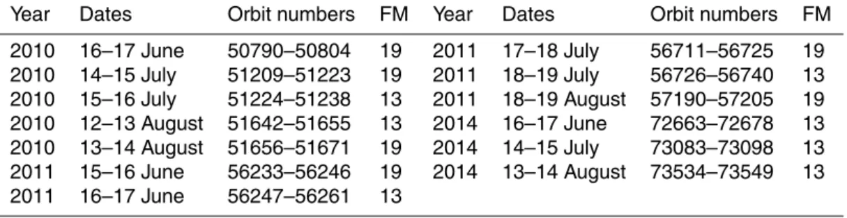
The Odin satellite and its instruments have many different modes of operation. In this study we use measurements taken in a special “tomographic” mode. These mea-surements were performed during three consecutive days in each of June, July and August 2010, 2011 and 2014, though only the measurements from 2010 and 2011 were considered for this study (see Table 1). In this mode the two instruments are set

15

to only scan the atmosphere at altitudes between 75 and 90 km to specifically target the summer mesopause. The tomographic mode is activated as the satellite crosses the equator, and measurements are made across the Northern Hemisphere. Figure 1a shows the coverage of the SMR tomographic mode during one day. As can be seen from the figure, large parts of the Northern Hemisphere is sampled by Odin over the

20

course of a day.

Since the tangent altitudes of the tomographic mode are limited to 75–90 km, the distance between each scan through the atmosphere is reduced from 1000 to 200 km, compared to previous Odin measurements of water vapour in the mesopause (Lossow et al., 2007). The shorter distance between scans means that the line-of-sight through

25

(7)

AMTD

7, 11853–11900, 2014

from Odin-SMR

Title Page

Tables Figures

◭ ◮

Back Close

Full Screen / Esc

Discussion

P

a

per

|

Discussion

P

a

per

|

Discussion

P

a

per

|

Discussion

P

a

per

|

can clearly be seen. The line-of-sight overlap means that in order to optimally retrieve information from these measurements, a tomographic retrieval approach should be used, hence the name “tomographic” mode.

2.2 SMR

This paper focuses on the tomographic mode measurements made by SMR. It

mea-5

sures radiation in five bands at around 118 and between 480–581 GHz, and can op-erate in several different frequency modes depending on the species of interest (Frisk et al., 2003). The tomographic mode uses either the A1 or B2 front-end, operating in the ranges 541–558 and 547–564 GHz, respectively, to measure the H₂O spectral line at 556.9 GHz. This is achieved by setting the LO frequency to 553.05 and 553.302 for

10

A1 and B2 frontends, respectively. The resulting frequency modes are labelled mode 19 and mode 13. A tunable Martin–Pupplet interferometer is used for single sideband (SSB) filtering. Pre-flight measurements show a nominal sideband suppression of bet-ter than 19 dB across the image band, with a maximum suppression of 35 dB (Eriksson et al., 2002). However, post-launch analysis of spectra indicates that the true

suppres-15

sion rather is 11–15 dB for the frequency modes used in this study.

The spectra are recorded using one of the two autocorrelator spectrometers among the SMR backends. Each autocorrelator has four sub-bands of 200 MHz, and provides a total bandwidth of 800 MHz. For mesospheric studies of the 557 GHz line only a part of full bandwidth is needed, and just the 200 MHz sub-band covering the line is used in

20

the retrieval process. The e_ffective channel resolution of the spectrometer is 2 MHz, and the channel separation 1 MHz. Furthermore, post-launch analysis of the instrument has revealed that the autocorrelators have problem measuring spectra with large dynamic ranges, i.e. large di_fferences in brightness temperature across the bandwidth of the instrument. This results in a low bias in the recorded brightness temperature, which

25

(8)

AMTD

7, 11853–11900, 2014

from Odin-SMR

Title Page

Tables Figures

◭ ◮

Back Close

Full Screen / Esc

Discussion

P

a

per

|

Discussion

P

a

per

|

Discussion

P

a

per

|

Discussion

P

a

per

|

The amount of noise in each channel is determined by the noise temperature of the system, the e_ffective channel resolution, and the integration time. For the frequency bands used in this study, SMR has a noise temperature of roughly 3000–3500 K. For the tomographic mode measurements, an integration time of 1.8 s is used. Due to the time used switching between calibration measurements and atmospheric

measure-5

ments SMR is only measuring the atmosphere about only half of the total time. Taking this into account, the resulting thermal noise (1σ) is in the order of 2.6 K for the mea-sured spectra.

To relate the measured radiation to a physical brightness temperature a calibration must be performed. The SMR measurements are calibrated by switching between the

10

cold sky (space) and the atmosphere, with a hot-load calibration performed at the end of each scan. In this study the newest version (V8) of the calibrated Odin spectra is used. This version was prepared during the autumn of 2013, and beside improving the treatment of known instrumental artefacts, it corrected an error related to the transition between orbits, which previously had made the tomographic observations unusable.

15

The vertical resolution of the measurements depends on the size and shape of the antenna pattern. For SMR the antenna is a 1.1 m Georgian telescope which provides a half power beam width better than 0.035◦(Frisk et al., 2003). This results in a vertical resolution at the tangent point of∼1.6 km. However, due to the telescope continuously scanning vertically during the integration time of 1.8 s the angular resolution is reduced

20

to 0.04◦(∼1.8 km) in the tomographic mode.

2.3 OSIRIS

In addition to presenting the results from the SMR tomographic mode retrievals, this pa-per also includes some comparisons with the PMC brightness retrieved from the optical spectrograph of OSIRIS. The spectrograph is a modified Erbert–Fastie grating

spec-25

(9)

AMTD

7, 11853–11900, 2014

from Odin-SMR

Title Page

Tables Figures

◭ ◮

Back Close

Full Screen / Esc

Discussion

P

a

per

|

Discussion

P

a

per

|

Discussion

P

a

per

|

Discussion

P

a

per

|

OSIRIS is aligned parallel to the horizon, and subtends a region 30 km wide and 1 km high at the tangent point.

To retrieve PMC properties from the scattered light, the measured radiation in the wavelength region of 302.8 to 305.9 nm is compared to a purely Rayleigh scattering background field calculated using the MSIS climatology. The di_fferences between the

5

measured and simulated spectra are then used as inputs to a tomographic retrieval scheme based on a modified version of the Multiplicative Algebraic Reconstruction Technique (MART, Degenstein et al., 2003). The retrievals return the scattering coe_ffi -cient of the clouds with a 330 km horizontal resolution and 1 km vertical resolution, and an accuracy of 4×10−11m−1str−1. For a detailed description of the observations and

10

retrieval process the reader is referred to Hultgren et al. (2013).

3 Retrieval methodology

To extract atmospheric data from the SMR measurements the optimal estimation method (OEM) is applied. ARTS (Atmospheric Radiative Transfer Simulator) is used as the forward model, and the retrieval procedure is implemented using a software

15

package accompanying ARTS. As previously mentioned, the overlapping lines-of-sight for the measurements allows for a tomographic retrieval approach. This means that a two dimensional (2-D) map of the atmospheric fields is retrieved, rather than sin-gle vertical profiles. The following section describes the forward model and retrieval procedure used in this study.

20

3.1 Forward model

3.1.1 General about ARTS

ARTS is a general purpose radiative transfer program, with a focus on supporting pas-sive microwave sounding techniques (Buehler et al., 2005). It is publicly available soft-ware. The second version of ARTS (Eriksson et al., 2011) allows simulations for 1-D,

(10)

AMTD

7, 11853–11900, 2014

from Odin-SMR

Title Page

Tables Figures

◭ ◮

Back Close

Full Screen / Esc

Discussion

P

a

per

|

Discussion

P

a

per

|

Discussion

P

a

per

|

Discussion

P

a

per

|

2-D or 3-D atmospheres, where the 2-D option is applied in this study. ARTS uses pressure as the main vertical coordinate. For 2-D, the observations are assumed to be performed along the orbit plane, and the horizontal coordinate can be seen as the angle along the orbit (AAO). For a hypothetical satellite having an orbit inclination of 90◦, the AAO could be set to match the geocentric latitude between−90 and₊90◦, but

5

ARTS allows the AAO to extend outside this range and the AAO zero point is a user choice.

The main di_fference between 1-D, 2-D and 3-D calculations is the ray tracing, the actual (clear-sky) radiative transfer is solved identically in all three cases. That is, after the atmospheric quantities along the propagation path are determined, the radiative

10

transfer along the path can be handled independently of the atmospheric dimension-ality. The treatment of weighting functions (columns of the Jacobian matrix) can be handled in basically the same way, and ARTS provides these functions for the same set of atmospheric quantities for 1-D, 2-D and 3-D. Atmospheric weighting functions are calculated using analytical expressions (ARTS also provides a pure numerical

op-15

tion), but these consider only local effects. For example, for temperature the hydrostatic equilibrium around each separate height is taken into account, but not how the hydro-static adjustment propagates to other altitudes. Furthermore, refraction is ignored in this study, as the effects are negligible for measurements limited to the mesosphere.

3.1.2 Grids

20

The atmosphere is modelled on a vertical grid stretching from 13.33 hPa (∼30 km) to 42 µPa (∼150 km). The grid has a height resolution of 100 m between 2.94 hPa (∼40 km) and 0.18 mPa (∼140 km), while above and below this a resolution of 250 and 500 m is used, respectively. The high vertical resolution of the grid is needed due to the fact that the water vapour line can saturate in the line centre, combined with the

25

strong vertical gradients in water vapour around the mesopause.

(11)

How-AMTD

7, 11853–11900, 2014

from Odin-SMR

Title Page

Tables Figures

◭ ◮

Back Close

Full Screen / Esc

Discussion

P

a

per

|

Discussion

P

a

per

|

Discussion

P

a

per

|

Discussion

P

a

per

|

ever, due to the large computational demands posed by the tomographic retrieval ap-proach, an entire orbit cannot be processed simultaneously on a desktop computer (32 GB RAM) unless data reduction techniques are applied. To keep the processing scheme simple, we have chosen not to apply any such techniques, but instead split the measurements into “batches” of 12 scans (∼150 spectra) covering ∼40◦ AAO (see

5

Fig. 1a). This results in the forward model horizontal grid for each batch covering±30◦ AAO (∼4500 km) around the centre of the batch with a resolution of 0.25◦ (∼30 km). Outside this area 16 additional gridpoints cover the AAOs up to±50◦AAO with a lower resolution to ensure that no errors arise from edge e_ffects.

3.1.3 Frequency grid and line parameters

10

ARTS is a line-by-line radiative transfer simulator, and for simulation of the 556.9 GHz water vapour transition we use a monochromatic frequency grid ranging from 556.5 to 557.5 GHz. The resolution is 100 kHz around the line centre (556.925 to 556.945 GHz) decreasing further away from the line centre reaching 100 MHz at the far end of the grid. In addition to the frequencies in the signal band, some frequencies are added in

15

the image band to accurately take into account influence of the sideband filtering. For the simulations in this study involving just a handful of transitions, absorption is best calculated for each point along the propagation paths (“on the fly” in ARTS terminol-ogy), as the option of using a pre-calculated look-up table is slower.

The line parameters for the water vapour line are taken from JPL and HITRAN2012.

20

JPL (Pickett et al., 1998) is used for the line position (556.9359877 GHz) and the line strength (229.8489 Hz/m2). HITRAN2012 (Rothman et al., 2013) is used for the pres-sure broadening coe_fficientγ_p. The coe_fficient is calculated asγ_p(p,T)₌pγ_air(T/T₀)n, where γ_air=31 362.45 Hz Pa−1 is the pressure broadening parameter, T the atmo-spheric temperature,T₀=296 K the reference temperature for the broadening

param-25

(12)

AMTD

7, 11853–11900, 2014

from Odin-SMR

Title Page

Tables Figures

◭ ◮

Back Close

Full Screen / Esc

Discussion

P

a

per

|

Discussion

P

a

per

|

Discussion

P

a

per

|

Discussion

P

a

per

|

3.1.4 Instrument

ARTS includes extensive support for incorporating instruments characteristics. Using the methodology introduced by Eriksson et al. (2002, 2006), monochromatic pencil beam spectra are combined, taking into account the response of antenna, mixer side-bands and spectrometer, to simulate final sensor brightness temperatures. For this

5

study, the modelled antenna pattern is based on the measurements of the SMR an-tenna system, the single sideband filter is modelled as a flat function with a sideband suppression of 14 dB, and the spectrometer backend channel response is based on a theoretical model of the spectrometer.

3.2 Retrieval

10

3.2.1 General OEM

In the optimal estimation method the retrieved state vector, ˆx, is the one minimising the a posteriori error, based on the known, or assumed, properties of the variations of the atmosphere and errors in the observation (Rodgers, 2000). Due to the non-linearity of the retrievals in this study an iterative Levenberg–Marquard method is applied. The

15

state vector of iterationi+1 from the OEM method is then given by

ˆ

x_i₊₁₌xˆ_i₊h(1+γ)S_a−1+(KT_iS−_ǫ1K_i)i−1hKT_iS−_ǫ1(y−f(x_i))−S−_a1(x_i−x_a)i, (1)

whereS_a and S_ǫ are the covariance matrices for the apriori state vector, x_a, and the thermal noise in the measurement given byy.K_i is the Jacobian matrix calculated us-ing the forward model of iterationi,f(x_i).γ is the Levenberg–Marquard parameter. It

20

(13)

itera-AMTD

7, 11853–11900, 2014

from Odin-SMR

Title Page

Tables Figures

◭ ◮

Back Close

Full Screen / Esc

Discussion

P

a

per

|

Discussion

P

a

per

|

Discussion

P

a

per

|

Discussion

P

a

per

|

tions, normalised by the apriori covariance, is is less than 0.01. For most cases this is achieved after 7–10 iterations, and the final normalised costs are between 0.9–1.1.

3.2.2 The state vector

The state vector contains all the variables to be retrieved, and in this study the state vector consists of the amount of atmospheric water vapour relative to the apriori (H₂O),

5

atmospheric temperatures in Kelvin (T) and some instrument variables. These vari-ables are a baseline fit, a frequency shift and a fit of the pointing error. The instrumental baseline arises due to standing waves in the receiver, and to fit this, a first order poly-nomial is fitted to each spectrum (P₀,P₁). The exact positioning of the LO frequency has some uncertainty. This is fitted with a single frequency fit (∆F) across each batch.

10

Finally there is an uncertainty in the pointing of the antenna, and a single pointing o_ffset (∆θ) is retrieved across the batch.

The total state vector is given by combining all the sub vectors

x₌[H₂O,T,∆F,∆θ,P₀,P₁]T. (2)

For the atmospheric fields (H₂O, T) the elements are sorted first by altitude then by

15

latitude and the retrieval grid covers altitudes between 316 Pa (∼40 km) to 0.75 mPa (∼130 km) with an altitude resolution of 1 km above 17 Pa (∼60 km) and a resolution of 2 km below. The horizontal retrieval grid covers 50◦ AAO centred around the batch with a resolution of 0.5◦.

3.2.3 Apriori values

20

For each state vector variable an apriori value must be given. For the atmospheric variables, these are given as two dimensional fields across the retrieval grid. For wa-ter vapour, an apriori profile constant with latitude and time was chosen. Using such a fixed apriori profile makes it easier to ensure that the structures seen in the retrieved water vapour field actually come from the measurements, rather than the apriori field.

(14)

AMTD

7, 11853–11900, 2014

from Odin-SMR

Title Page

Tables Figures

◭ ◮

Back Close

Full Screen / Esc

Discussion

P

a

per

|

Discussion

P

a

per

|

Discussion

P

a

per

|

Discussion

P

a

per

|

The apriori profile is based on a climatology of water vapour from the MLS instrument on board the AURA satellite. Taking the mean of the MLS water vapour concentra-tions from June, July and August for latitudes above 60◦, the profile shown in Fig. 2 is obtained.

For temperature the MSISE-90 model (Hedin, 1991) is used as the apriori value.

5

The model gives the mean temperature for each month as a function of latitude and pressure, covering pressures from 1013 hPa (∼0 km) to 5.7×10−4Pa (∼130 km). Fur-thermore, the MSIS90E-90 climatology is used for the pressure–altitude relationship for the retrievals. However, since temperature, pressure and altitude are closely interlinked through the hydrostatic equilibrium (HSE), the pressure–altitude relationship must be

10

adjusted during the retrieval to ensure a consistent relationship between the three vari-ables. This is done by using the MSISE-90 model to find the geometrical altitude cor-responding to a pressure level of 2.9 Pa, and the correcting the pressure–altitude rela-tionship for the other pressure levels by assuming HSE in the retrieved atmosphere.

For the instrumental variables, the apriori assumption is that the measurements are

15

(15)

AMTD

7, 11853–11900, 2014

from Odin-SMR

Title Page

Tables Figures

◭ ◮

Back Close

Full Screen / Esc

Discussion

P

a

per

|

Discussion

P

a

per

|

Discussion

P

a

per

|

Discussion

P

a

per

|

3.2.4 Apriori covariance

The optimal estimation method requires, in addition to apriori values, a covariance matrix to be created for the state vector variables. The total covariance matrix is set to a block diagonal matrix with the covariance matrix for each variable in each block

S_a= 

          

SH2O

a 0 0 0 0 0

0 STemp_a 0 0 0 0

0 0 σa∆F 2

0 0 0

0 0 0 σa∆θ

2

0 0

0 0 0 0 SP_a0 0

0 0 0 0 0 SP_a1



          

. (3)

5

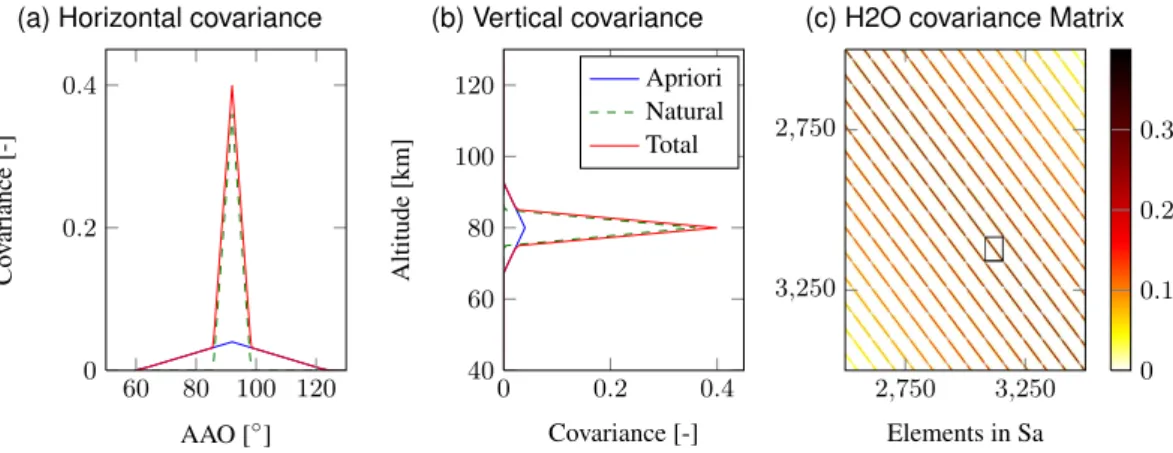
For the atmospheric fields the apriori covariance matrices are matrices with non zero elements far from the diagonal due to correlation in the errors in the apriori atmosphere and natural variation across the 2-D grid. In this study, following Eriksson (2000), we use two terms to describe this covariance. One term represents the large scale un-certainty of the apriori mean, whereas the other describes the smaller scale natural

10

variations in the mesosphere (i.e. deviations from the true mean state). The apriori un-certainty for each of these terms is di_fferent. For water vapour and temperature, the SDs for the uncertainty in the apriori mean are set to 20 % and 5 K, and the natural variability around the means are set to 20 % and 10 K, respectively.

The spatial correlations of the uncertainty for these terms are also di_fferent, and to

15

(16)

AMTD

7, 11853–11900, 2014

from Odin-SMR

Title Page

Tables Figures

◭ ◮

Back Close

Full Screen / Esc

Discussion

P

a

per

|

Discussion

P

a

per

|

Discussion

P

a

per

|

Discussion

P

a

per

|

mean). The covariance for water vapour in the horizontal and vertical directions of the two terms and the total covariance is shown in Fig. 3a and b.

Assuming that the correlation in the two dimensions are independent (separable), the total correlation is given as the product of the two, and the complete covariance matrix can be calculated. A part of this matrix for water vapour is shown in Fig. 3a.

5

It can be seen that the matrix has a block structure, where each blockSi_a,j, indicated by the black square in the figure, is the covariance matrix covering all altitudes at one AAO, and the off-diagonal blocks are the vertical covariance matrix multiplied by the correlation between the different AAOs.

For the instrumental variables the covariance matrices are pure diagonal matrices (or

10

scalars). For the baseline polynomial fits uncertainty is set to 4 and 2 K for the zeroth and first order respectively. For the frequency fit the covariance matrix is simply a scalar with an assumed uncertainty of 100 kHz, whereas the pointing error the uncertainty is set to 0.001◦. The strict regularisation on the pointing o_ffset is needed to prevent the non-linear retrievals from converging to unrealistic results.

15

4 Results

4.1 A simulated case

In order to illustrate the viability of the tomographic methodology, a simulated retrieval was performed. In this way the sensitivity of the retrievals to changes in water vapour and temperature can be investigated. The mean temperature and water vapour

re-20

trieved from the tomographic measurements was used as the atmospheric apriori in the simulation. Since the purpose of this study is to look at small scale variations of water vapour and temperature around PMCs, a water vapour enhancement of 50 % was simulated in a small region of the atmosphere (200 km×2 km), and a set of simu-lated measurements were then generated using this atmosphere. This test atmosphere

25

(17)

AMTD

7, 11853–11900, 2014

from Odin-SMR

Title Page

Tables Figures

◭ ◮

Back Close

Full Screen / Esc

Discussion

P

a

per

|

Discussion

P

a

per

|

Discussion

P

a

per

|

Discussion

P

a

per

|

of the methodology. The retrieval was performed as described in Sect. 3. However, since the convergence criterion of the retrievals is based on changes from the apri-ori atmosphere, and only small deviations from the apriapri-ori atmosphere were simulated (compared to deviations expected in the real case), a stricter convergence criterion of 0.0001 had to be used in the simulated case, compared to 0.01 in the real retrievals.

5

Furthermore, no noise was added to the simulated spectra, but the simulated retrievals were done using a noise covariance matrix describing a thermal noise with aσof 2.6 K. Figure 4a shows the retrieved water vapour, relative to the apriori atmosphere, from the simulated retrieval. The small area where the simulated atmosphere has enhanced water vapour is shown by the black contour, whereas the retrieved water vapour is

10

shown by the coloured contours. It is clear from the results that the retrievals reproduce the water vapour enhancement, though some smoothing is seen as the area enhanced in the retrieved data is slightly larger than than that of the simulated atmosphere.

In addition to water vapour, the tomographic retrieval returns the temperature field of the atmosphere. Due to the nature of the measurement method, these two retrieved

15

quantities will not be independent of each other. As a result an increase in water vapour will have some influence on the retrieved temperature field, and Fig. 4b shows the change in retrieved temperature as a result of the water vapour enhancement. The temperature retrievals were affected by the enhancement in water vapour, and varia-tions of±3 K are seen in the retrieved data around the water vapour enhancement.

20

To test the temperature retrievals, another simulation was set up. In this simulation (not shown) the water vapour distribution was set equal to the measured mean, and the temperature was perturbed by reducing it by 5 K in the 200 km×2 km area. For the temperature the perturbed area was reproduced in the correct position, albeit with some smoothing. The influence on a change in temperature on the retrieved water

25

vapour field was small, with a change of only 2 % in the retrieved water vapour within the perturbed area, and no change outside of it.

(18)

AMTD

7, 11853–11900, 2014

from Odin-SMR

Title Page

Tables Figures

◭ ◮

Back Close

Full Screen / Esc

Discussion

P

a

per

|

Discussion

P

a

per

|

Discussion

P

a

per

|

Discussion

P

a

per

|

interest. The simulated tests also illustrate some of the errors that can arise from the retrievals. A further discussion of the uncertainties and errors of the retrievals can be found in Sect. 5.

4.2 Result from a real case

To exemplify the results of the tomographic measurements, two orbits (51221 and

5

51226) recorded on 15 July 2010 are selected as example orbits. Orbit 51221 is se-lected as collocations between Odin-SMR and both ACE-FTS and AIM-SOFIE can be found along this orbit. Orbit 21226 is used since it is an orbit recorded soon after using the other frontend.

Figure 5 shows some example spectra from orbit 51226 at different tangent altitudes.

10

The saturation of the line at the lower altitudes is seen, as the brightness temperature of the line centre is lower than the line wings, reflecting the negative temperature gra-dient of the mesosphere. The spectra fitted by the retrievals are shown as dashed lines showing how they reproduce the general shape and amplitude of the measured spectra. To get a better view of the fit, the residuals from all spectra in orbit 51226 are

15

shown in Fig. 5b. Ideally the residuals should be white noise with a SD equal to that of the thermal noise of the receiver. For most of the spectrometer channels this is true, however, for the channels closest to the line centre some non-white noise can be seen. This arises due to instrumental errors not represented in the forward model, and as such will not be fitted to the spectra.

20

4.2.1 Water vapour and temperature

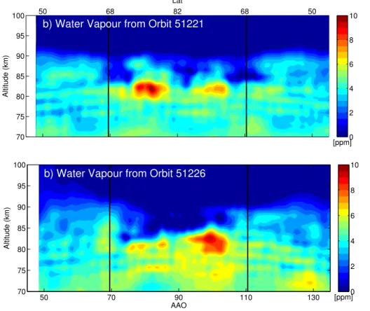
Figure 6 shows the retrieved water vapour for the two selected orbits. The retrieved fields cover latitudes (top x axis) from ∼50 up to 82◦N and then down to ∼50◦N on the other side of the pole. The vertical distribution of water vapour shows high concentration (>4 ppm) up to∼85 km where it quickly drops down to values between

25

(19)

AMTD

7, 11853–11900, 2014

from Odin-SMR

Title Page

Tables Figures

◭ ◮

Back Close

Full Screen / Esc

Discussion

P

a

per

|

Discussion

P

a

per

|

Discussion

P

a

per

|

Discussion

P

a

per

|

summer mesosphere where water vapour is brought up from the lower altitudes by the mesospheric overturning circulation and removed by photodissociation as it reaches the mesopause.

The latitudinal distribution of water vapour shows generally higher concentrations towards the pole than at lower latitudes, and both orbits have large areas with

wa-5

ter vapour concentrations above 10 ppm between 70 and 80◦N. Figure 6b in partic-ular shows the water vapour concentrated in two areas at 80 and 100◦ AAO, while in Fig. 6a the concentration is highest at 100◦AAO. These areas arise as a result of atmo-spheric dynamics combined with the redistribution of water vapour due to the presence of PMCs. Another feature of both figures is the wave like oscillating structures in the

10

vertical directions seen across the entire orbit. These oscillations are retrieval artefacts due to thermal noise in the measurements, and do not represent the true structure of the atmosphere.

Below 80 km there are significant di_fferences between the two orbits. Figure 6b shows less water vapour overall, and large amount of water between 65 and 105◦

15

AAO is not present compared to Fig. 6a. Comparing several other orbits show that this is probably due to instrumental di_fferences between the two frontends rather than a physical change in the real atmosphere. The consequences and implication of this will be elaborated further in Sect. 5.3, where the results are compared to other satellite instruments.

20

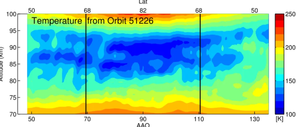
Figure 7 shows the temperature field retrieved from orbit 51226. The retrieved perature shows a mesopause altitude around 90 km with the lowest mesopause tem-peratures (∼115 K) closest to the poles. This is once again due to the mesospheric overturning circulation, with the faster ascending air over the pole causing a stronger cooling than at lower latitudes.

(20)

AMTD

7, 11853–11900, 2014

from Odin-SMR

Title Page

Tables Figures

◭ ◮

Back Close

Full Screen / Esc

Discussion

P

a

per

|

Discussion

P

a

per

|

Discussion

P

a

per

|

Discussion

P

a

per

|

5 Discussion

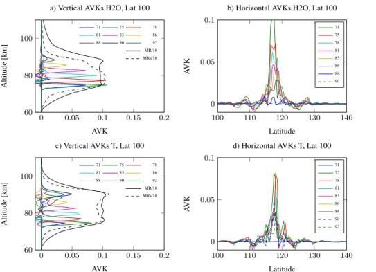
5.1 Averaging kernels

Spatial resolution of retrieved data is usually described by the rows of the averag-ing kernel matrix (AVKs). Each element in the averagaverag-ing kernel matrix,A_{i j}, gives the change in the retrieved state vector element ˆx_i from a change in the true state vector

5

element x_j, and the spatial resolution of the retrievals can be described with the full width at half maximum (FWHM) of the AVKs.

For non-linear retrievals the AVKs will depend on the atmospheric state, and will vary between measurements. Thus, in order to give the most representative picture of the capabilities and limitation of the retrievals, we have chosen to show the AVKs

10

using the mean retrieved state from all the measurements. The AVKs are calculated assuming that the Levenberg–Marquard parameter is zero at the final iteration, i.e. we present the AVKs for the linear retrieval around the mean retrieved atmospheric state (Ceccherini and Ridolfi, 2010). This is valid for most of the retrieved cases, although for some batches the Levenberg–Marquard parameter does not reach zero, but remains

15

between 1 to 4 during the final iterations. For these batches, the AVKs presented here should be regarded as an approximation, rather than a perfect characterisation of the performance of the retrievals.

5.1.1 Spatial resolution

Figure 8 shows the calculated horizontal and vertical averaging kernels. The vertical

20

AVKs show a clear separation between the different altitudes for both water vapour and temperature, and between 75–88 km and the vertical resolution is 2.5 km. The horizontal AVKs for di_fferent altitudes are shown in left panels of Fig. 8. The horizontal AVKs have a more jagged appearance than the vertical ones, and their peaks do not always align with the AAO which they represent. However, for the altitudes between

25

(21)

AMTD

7, 11853–11900, 2014

from Odin-SMR

Title Page

Tables Figures

◭ ◮

Back Close

Full Screen / Esc

Discussion

P

a

per

|

Discussion

P

a

per

|

Discussion

P

a

per

|

Discussion

P

a

per

|

AVKs do oscillate, and a secondary peak is seen∼4◦on either side of the main peak. At higher altitudes (83 and 85 km) the main peak is less pronounced and the AVK is a flatter with FWHM of up to 5◦. This shows that the best horizontal resolutions are for the altitudes around 80 km, with a deteriorating resolution as the altitude increases.

5.1.2 Measurement response

5

The measurement response (MR) of the retrievals gives an indication of how sensitive the retrievals are to large scale changes in the true atmosphere, and is calculated by summing the AVKs along each row over all columns corresponding to the retrieved variable (Baron et al., 2002). The measurement response (MR) for water vapour and temperature are shown as solid lines in Fig. 8a and c respectively. The plotted value

10

is the measurement response/10, and altitudes with values greater than∼0.6 are ar-eas where the mar-easurement information is considered to contribute significantly to the retrieved data. This area covers the altitudes between 75 and 90 km. The retrieved large scale changes, however, have large uncertainties. These errors come from the fact that there is little information about the ambient pressure of the atmosphere in the

15

measured radiation. The result of this is that errors in the pointing of the satellite as well as errors in the altitude of the HSE reference pressure level of the retrievals can lead to large errors in the retrieved water vapour mixing ratio (see Sect. 5.2). An alternative measurement response is therefore calculated to show the sensitivity of the retrievals to smaller scale changes in the atmosphere. It is calculated by summing over the AVK

20

(22)

AMTD

7, 11853–11900, 2014

from Odin-SMR

Title Page

Tables Figures

◭ ◮

Back Close

Full Screen / Esc

Discussion

P

a

per

|

Discussion

P

a

per

|

Discussion

P

a

per

|

Discussion

P

a

per

|

5.2 Errors

There are several possible sources of errors in the retrievals. Random errors come from thermal noise in the measurements (retrieval noise), from the limited resolution of the measurements (smoothing error), and pointing error in the satellite. Additionally, the results have systematic errors related to uncertainties in modelling of the instrument,

5

modelling of the atmosphere, and uncertainties in the spectral line parameters. Just as with the averaging kernels, the effect of uncertainties and errors will depend on the true atmospheric profile. Thus, to give an indication of the average error expected in the retrievals, the error analysis is based around a case linearised around the mean retrieved state of the measurements.

10

The smoothing error and retrieval noise are calculated using the covariance ma-trices, S_a and S_ǫ respectively, as described in Rodgers (2000). The retrieval noise is∼0.5 ppm for water vapour and 3 K for temperature. An accurate estimation of the smoothing error, however, requires that the atmospheric covariance matrix is known with certainty, which is not the case for the tomographic retrievals. As such we will not

15

use the smoothing errors for the error analysis, but rather consider the retrieved re-sult as the smoothed version of the true atmosphere, with the resolution given by the averaging kernels.

For the systematic errors, their influence is estimated by performing a simulated retrieval on the mean retrieved state with the forward model perturbed to the±1σ

esti-20

mate of the investigated parameter. The parameters investigated are the linestrength,

I₀, which is perturbed±2 %, based on the JPL uncertainty, the pressure broadening pa-rameter,γ, which is perturbed 5 %, based on di_fferences between the measurements reported in Seta et al. (2008). Errors in the altitude of the HSE reference pressure level (2.9 Pa),P ressure, is estimated by moving the pressure level±2 km, based on

25

(23)

AMTD

7, 11853–11900, 2014

from Odin-SMR

Title Page

Tables Figures

◭ ◮

Back Close

Full Screen / Esc

Discussion

P

a

per

|

Discussion

P

a

per

|

Discussion

P

a

per

|

Discussion

P

a

per

|

instrumental parameters investigated are an o_ffset in the pointing of ±0.02◦ (Lossow et al., 2007), and uncertainties in the sideband suppression of±2 % (11–15 dB).

It should be noted that the presence of PMCs will not affect the retrieval of water vapour and temperature from SMR. The radiance emitted from ice particles is in the order of 0.1 K, and will be very uniform across the bandwidth of the spectrometer. As

5

such, it will be completely overshadowed by any baseline in spectrometer, and thus corrected for in the polynomial baseline fit performed on each spectrum.

Figure 9 shows the random and systematic errors estimated around the mean at-mospheric state. The plotted value,∆E, is the mean absolute value of the difference between the perturbed,x(±σ), and unperturbed,x(0), retrievals given by

10

∆E=|x(σ)−x(0)|+|x(−σ)−x(0)|

2 . (4)

The two largest sources of uncertainties in the retrievals are the pressure–altitude relationship (red line) and errors in pointing of the satellite (cyan line). The reason for this is that the weighting function for a change in water vapour is similar to the weight-ing function from the changweight-ing of the pointweight-ing angle of the satellite, or from a change

15

in ambient pressure at di_fferent altitudes. Since the water vapour line is dominated by Doppler (compared to pressure-) broadening at the observed altitudes, and the number density of molecules decrease exponentially with altitude, any pointing error (or errors in altitude of the HSE reference point) will give rise to a large scale change in the re-trieved water vapour mixing ratio, and vice versa. The errors arising from assuming the

20

wrong altitude of the 2.9 Pa pressure level can be adjusted for by ensuring that compar-isons to other instruments or models are done with respect to a common pressure vs. altitude profile, in effect comparing number density- rather than mixing ratio profiles. If this is done, the estimated systematic error from this uncertainty is lowered to∼2 ppm (red-dashed curve in Fig. 9).

25

(24)

AMTD

7, 11853–11900, 2014

from Odin-SMR

Title Page

Tables Figures

◭ ◮

Back Close

Full Screen / Esc

Discussion

P

a

per

|

Discussion

P

a

per

|

Discussion

P

a

per

|

Discussion

P

a

per

|

vapour field retrieved in each orbit, and not the variations around this field. For these variations the other systematic errors will dominate, and as these are on the order of the noise in the data, we conclude that the measurements reliably can retrieve these variations, despite the poor accuracy of the mean field. It should also be noted that the systematic errors introduced from the pointing and pressure uncertainties do not

5

necessarily lead to a bias as both errors may vary across the measurement period.

5.3 Comparison with other measurements

As a final test of the ability of the observations to retrieve water vapour and tem-perature, the results are compared to measurements from other satellite instruments. The solar occulting instruments Atmospheric Chemistry Experiment-Fourier Transform

10

Spectrometer (ACE-FTS) on board the SCISAT satellite (Bernath et al., 2005) and So-lar Occultation for Ice Experiment (SOFIE) on board the AIM satellite (Russell et al., 2009) provide water vapour and temperature measurements with high vertical reso-lution in the area covered by the tomographic retrievals during the time period of the tomographic measurements.

15

ACE-FTS is a Fourier transform spectrometer which measures solar radiation be-tween 750–4400 cm−1 and retrieves water vapour and temperature profiles (Boone et al., 2005) between 5–90 km with an altitude resolution of 3–4 km and a precision of

∼300 ppbv for water vapour (statistical fitting error and “form-factor” error Boone et al., 2013) and∼2 K for temperature (comparison to LIDAR Sica et al., 2008). In this study

20

we use version 3.0 of the water vapour data (Boone et al., 2013), which provides data during July 2010 in the time period covered by tomographic retrievals.

SOFIE uses differential absorption spectroscopy at eleven different wavelengths be-tween 0.292 to 5.316 µm to determine the temperature and the atmospheric composi-tion. It retrieves water vapour and temperature between 20–95 km with a vertical

reso-25

(25)

AMTD

7, 11853–11900, 2014

from Odin-SMR

Title Page

Tables Figures

◭ ◮

Back Close

Full Screen / Esc

Discussion

P

a

per

|

Discussion

P

a

per

|

Discussion

P

a

per

|

Discussion

P

a

per

|

this study we use version 1.2 of the data which covers the entire time period of the tomographic Odin measurements.

The measurements are collocated by finding the retrieved SMR profile at the latitude of FTS/SOFIE measurements and comparing it to the closest (spatially) ACE-FTS/SOFIE during the same day. Due to the di_fferent orbits of the satellites there are

5

some distance between the collocated measurements, but 90 % of the collocations are within 350 km. This means that some differences between the profiles due to natural variability should be expected. Another reason for discrepancies between the measure-ments is that, while SOFIE and ACE-FTS performs measuremeasure-ments at ∼23:00 LT and

∼01:00 LT due to their solar occultation technique, SMR measurements are performed

10

around 17:00 LT. Furthermore, the occultation measurements are made perpendicular to the orbit, i.e. east–west, while SMR measures along the orbit i.e. north–south. The differences due to sampling different air, however, should largely average out (except possible diurnal variations) when comparing data over the entire PMC season.

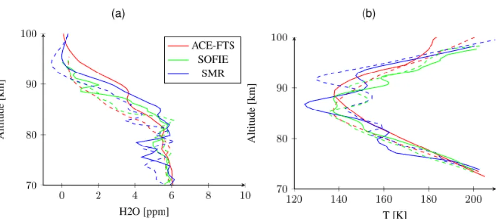
The result from SMR Orbit 51226 (15 July 2010) is compared to AIM-SOFIE and

15

ACE-FTS in Fig. 10. The position of the collocations are showed by the vertical black lines in Fig. 6. The solid and dashed lines in Fig. 10 are the collocations at AAO₌70◦ and AAO₌110◦respectively. For water vapour the agreement between the instruments is good, but SMR seems to show too low values below 80 km. Looking at the longitu-dinal di_fferences all three instruments measure lower concentrations of water vapour

20

between 80–88 km at 81◦E (dashed lines) compared to 63◦W. The retrieved tempera-ture of the three instruments have larger differences. For the profile measured at 63◦W (solid lines) SMR and SOFIE places the mesopause at the same altitude (88 km), while the profile from ACE-FTS shows the mesopause at 90 km. SMR does however mea-sure a significantly lower mesopause temperature (<130 K) than the two other

instru-25

(26)

tomo-AMTD

7, 11853–11900, 2014

from Odin-SMR

Title Page

Tables Figures

◭ ◮

Back Close

Full Screen / Esc

Discussion

P

a

per

|

Discussion

P

a

per

|

Discussion

P

a

per

|

Discussion

P

a

per

|

graphic measurements successfully can retrieve water vapour and temperature struc-tures in the area of interest.

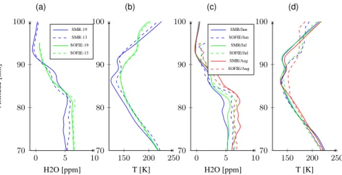
To look at the systematic errors in the tomographic retrievals, the mean of all mea-surements collocated with SOFIE is analysed. A total of 198 collocations are investi-gated, and Fig. 11a and b shows the result of this comparison with respect to each of

5

the two frequency modes of SMR. The measurements using mode 19 show a low bias compared to SOFIE in both water vapour (>1 ppm) and temperature (>20 K). These biases are also seen in the measurements using mode 13, but they are significantly smaller. The estimated accuracy of SOIFE is∼5 %/0.8 K at 80 km and 15 %/9.9 K at 95 km for water vapour (Rong et al., 2010) and temperature (Stevens et al., 2012)

re-10

spectively. Taking this into account the agreement between SMR and SOFIE is good for mode 13, but not for mode 19. Above 90 km a large difference in mean temperature can be seen. However, this is probably due to a known high bias in SOFIE (Stevens et al., 2012).

The comparison of the mean profiles can be extended by looking at the mean profile

15

from each month for SOFIE and SMR. Figure 11c shows the mean water vapour pro-files from both instruments for June, July and August averaged over 2010 and 2011. Only the collocations from the frequency mode 13 measurements are used. In June, SOFIE (blue-dashed line) shows a higher water vapour concentration below 82 km than SMR (blue line), while in August (red lines) the reverse is true. The reason for the larger

20

seasonal variation in water vapour in SMR is unknown, but it could be linked to sys-tematic errors in the pressure apriori used for the retrievals. The mean temperature (Fig. 11d) is very similar for both SMR and SOFIE for June and July, while for August SOFIE retrieves a much higher mesopause temperature (155 K) compared to SMR (140 K).

25

(27)

AMTD

7, 11853–11900, 2014

from Odin-SMR

Title Page

Tables Figures

◭ ◮

Back Close

Full Screen / Esc

Discussion

P

a

per

|

Discussion

P

a

per

|

Discussion

P

a

per

|

Discussion

P

a

per

|

pressure information in the SMR measurements. However, the main differences seen in the comparisons do not depend on this rescaling.

In conclusion, the overall the agreement between the SMR tomographic measure-ments and the two solar occulting instrumeasure-ments are within the accuracy estimations from Sect. 5.2 for the measurements made with frequency mode 13. For the measurements

5

made with mode 19 however there is a clear systematic low bias in both water vapour and temperature. The measurements from SMR also show a larger seasonal variance of water vapour, with lower concentrations than SOFIE in June and higher concentra-tions in August.

5.4 Comparison to OSIRIS

10

As previously mentioned, one of the reason for doing the tomographic SMR measure-ments is that measuremeasure-ments by OSIRIS are able to retrieve PMC coverage at the same time. Figure 12 shows some example results combining measurements from both the instruments. The left panels show the water vapour distribution around PMCs from two di_fferent orbits recorded on 15 July 2010. The white contours show the volume

scat-15

tering coefficient from the PMCs measured by OSIRIS. The most striking feature is the strong depletion of water vapour above the clouds. This is seen particularly well above each of the three cloudy areas at 80, 90 and 100◦ AAO in Fig. 12c. At 82 km, there are areas with higher water vapour concentrations between the clouds, indicating possible cloud deposition. In Fig. 12a the water vapour is concentrated in a single area at 100◦

20

AAO. The reason for this feature cannot be explained by looking at the cloud distri-bution alone, but probably arises as a combination of air movement as well as cloud formation and particle sedimentation.

The atmospheric temperatures are shown in the rightmost panels in Fig. 12. In gen-eral, the existence of clouds seem to correlate with the cold areas at 82 km. In particular

25

(28)

pene-AMTD

7, 11853–11900, 2014

from Odin-SMR

Title Page

Tables Figures

◭ ◮

Back Close

Full Screen / Esc

Discussion

P

a

per

|

Discussion

P

a

per

|

Discussion

P

a

per

|

Discussion

P

a

per

|

trate into areas of higher temperature (>150 K), once again explaining these intrusions require further analysis taking into account both cloud microphysics and the dynamics of the atmosphere.

6 Conclusions

Water vapour and temperature have been measured around PMC by several

ground-5

and satellite based instruments in the past, but until now, simultaneous measurements of water vapour, temperature and PMC with a large geographical coverage and rela-tively good vertical and horizontal resolution have not existed. During the arctic sum-mers of 2010, 2011 and 2014 the Odin satellite made a set of measurements with both Odin-SMR and Odin-OSIRIS to obtain such data.

10

In this paper we present the measurements of water vapour and temperature carried out by the SMR instrument. A tomographic retrieval approach based on the optimal estimation method is applied, and is described in detail. An error analysis was per-formed to investigate possible sources of errors in the retrieved data, and the data was compared to two other satellite instruments for quality assurance.

15

The largest source of errors in the data comes from the uncertainty in the satellite pointing and the altitude of the 2.9 Pa pressure level, which is used as the reference level to adjust the atmosphere to remain in HSE. These large uncertainties indicate that the tomographic retrievals have limited capability to retrieve the mean water vapour mixing ratio for each orbit. However, the retrieved variations of water vapour around this

20

mean are significantly less affected by these errors, and can retrieved by the measure-ments with reasonable accuracy.

Inspecting tomographic retrievals done in di_fferent frequency modes revealed dis-crepancies between measurements frequency mode 19 and 13. By comparing the results to collocated AIM-SOFIE measurements, we conclude that the best results are

25