Electoral rules, political competition and fiscal spending: regression discontinuity evidence from brazilian municipalities

ELECTORAL

RULES,

POLITICAL

COMPETITION

AND

FISCAL

SPENDING:

REGRESSION

DISCONTINUITY

EVIDENCE

FROM

BRAZILIAN

MUNICIPALITIES

M

C

J

M.

P.

M

S

F

Outubro

de 2009

T

Te

ex

xt

to

os

s

p

p

a

a

ra

r

a

D

Di

is

sc

cu

us

ss

sã

ão

o

TEXTO PARA DISCUSSÃO 208 • OUTUBRO DE 2009 • 1

Os artigos dos Textos para Discussão da Escola de Economia de São Paulo da Fundação Getulio

Vargas são de inteira responsabilidade dos autores e não refletem necessariamente a opinião da

FGV-EESP. É permitida a reprodução total ou parcial dos artigos, desde que creditada a fonte.

E

R

,

P

C

F

S

:

R

D

E

B

M

MARCOS CHAMON†,JOÃO M.P.DE MELLO‡ AND SERGIO FIRPO¥

October 2008

Abstract

We exploit a discontinuity in Brazilian municipal election rules to investigate whether

political competition has a causal impact on policy choices. In municipalities with less than

200,000 voters mayors are elected with a plurality of the vote. In municipalities with more

than 200,000 voters a run-off election takes place among the top two candidates if neither

achieves a majority of the votes. At a first stage, we show that the possibility of runoff

increases political competition. At a second stage, we use the discontinuity as a source of

exogenous variation to infer causality from political competition to fiscal policy. Our second

stage results suggest that political competition induces more investment and less current

spending, particularly personnel expenses. Furthermore, the impact of political competition is

larger when incumbents can run for reelection, suggesting incentives matter insofar as

incumbents can themselves remain in office.

KEY WORDS: Electoral Systems; Strategic Voting; Political Competition; Regression

Discontinuity; Fiscal Spending.

JEL CODES: H72; D72; C14; P1

§

We would like to thank Helios Herrera, Leonardo Rezende, Filipe Campante, Alexandre Samy, Claudio Ferraz, and seminar participants at EESP-FGV, PUC-Rio and IPEA-RJ for useful comments. Edson Macedo, Mariano Lima, João Pedro Borges and Julia Folescu provided excellent research assistance. Usual disclaimer applies.

†

International Monetary Fund and BREAD: mchamon@imf.org. The views expressed in this paper are those of the authors and should not be attributed to the International Monetary Fund.

‡

Departamento de Economia, PUC-Rio: jmpm@econ.puc-rio.br.

¥

“How an excess of political stability can get in the way of good government”

The Economist, May 17th, 2008 commenting on the mishaps of the

Concertación, the Chilean long-standing governing coalition.

1. Introduction

It is well established that electoral rules have strong implications for the political

process. For example, plurality voting favors a two-party system (“Duverger’s Law”,

Duverger, 1954). By affecting party formation, different electoral rules induce different

levels of electoral competition. However, the effects of political competition on policy

choices are not well understood empirically. It is not surprising that the empirical link from

political competition to policy making can be elusive, as the two are simultaneously

determined. For example, we may observe a scenario where barriers to entry lead to low

competition and bad policies. We may also observe situations where a highly capable

incumbent discourages entry by challengers, and low competition coexists with good

policies. Although a growing body of evidence supports the view that competition improves

policy making,1 _{too little a barrier to entry may lead to instability, fragmentation and worse}

policies.2

In this paper we explore a unique discontinuity in the rules for Municipal elections in

Brazil, which provides a sharp identification of how lower political entry-costs can affect

policy outcomes. Our results indicate greater competition improves fiscal policy. Mayoral

elections in Brazil take place every four years, with the election rules varying depending on

the size of the electorate. Voting is mandatory. In municipalities with more than 200,000

registered voters elections are in a two-round system. A run-off between the first-round

winner and the runner-up takes place if the former receives less than 50% of valid votes. In

municipalities with less than 200,000 registered voters there is only one round with the

1

See, for example, Besley et al (2005), Besley and Case (1995), Rodgers and Rodgers (2000), and Besley and Case (2003).

2

winner being the one who gains the most votes. The 200,000 threshold rule provides an

exogenous and abrupt change in the voting system as a function of the electorate size. As

long as the electoral rules cause “political market” structure, it can be a source of exogenous

variation in the degree of competitiveness of the “political market”. This discontinuity

arguably provides the sharpest identification for the causal effect of political competition on

fiscal policy outcomes.

The link from electoral rules to political market structure is well established in the

literature.3 _{Most comparisons contrast majority and proportional systems, and why the latter}

favors multi-party structures. Nevertheless, similar arguments can be made for comparing

one-round with two-round majority elections. For example, consider a one-round election

and suppose that 60 percent of the electorate is left-leaning. If there is one left-leaning and

one right-leaning party contesting the election, the former should easily win. But if there are

two competing left-leaning parties, the right-leaning one may be able to achieve a plurality of

the vote. In this case, the third candidate would be a “spoiler,” and in a well functioning

system the two left-leaning parties should form a coalition and launch a single candidate. In a

two-round election, the presence of the third candidate should not affect the final outcome

and therefore we should expect a larger supply of candidates under that system.4,5

Methodologically, we use a regression-discontinuity design (RDD)6, which is known

for its very high internal validity as it exploits the exogenous variation that occurs around the

discontinuity point. Thus, it dispenses with concerns about unobserved heterogeneity driving

results. We show that there is a discrete and sizeable jump in voting concentration as function

of the electorate size and that this jump occurs at the 200,000 voter threshold. That is, there is

an abrupt increase in political competition for municipalities where the second round is

3

For example, Duverger’s Law, which is formally proved in Palfrey (1989).

4

Note that the presence of a run-off would not necessarily rule out a right-leaning party victory in this example. Suppose there are four left-leaning parties each of which receives 15 percent of the vote, and two right-leaning parties that receive 20 percent of the vote. Then, a run-off would take place with the two right-leaning parties.

5

The presence of a run-off is more likely to affect the outcome of the election when voters choose their first choice of candidate (sincere voting) than under strategic voting. The political economy literature has interest in sincere versus strategic voting because of their different implications for modeling. Some empirical evidence is available, mainly using structural modeling strategies. See Degan and Merlo (2007) and Merlo (2006).

6

present. Following the Political Science literature, we measure concentration both as the

number of effective candidates as well as the share of votes going to the third-placed or lower

candidates.7 _{Thus, the run-off reduces the “political market concentration” by encouraging}

more parties to enter and/or inducing sincere voting in the first round, thus turning the

political regime more competitive.

As we are concerned with the causal link from political competition to policy

outcomes we estimate how the exogenous change in political competition around the 200,000

voter threshold affects policy outcomes. The way we proceed is by using a weighted

instrumental variable regression where the dependent variables are policy outcomes (capital

and current expenses and construction of schools), the endogenous regressor is a measure of

political competition and the instrument a dummy variable that equals one if a municipality

has more than 200,000 voters and zero otherwise. The weights are decreasing functions of

distance between municipal electoral size and 200,000 voters. Thus, weights play an

important role in our IV strategy by augmenting the importance of observations around the

discontinuity.8

Finally, note that there is no reason to believe that municipalities right after

and before the discontinuity should have different fiscal policies beyond and above the effect

through political competition.

Our results indicate that a higher degree of political competition causes more capital

spending, less spending in current expenses, and more construction of schools. Most of the

estimated reduction in current expenditure takes place through lower payroll spending. In

contrast with previous works, we do not estimate the effect of political competition on the

size of government since in most municipalities the vast majority of expenditures are

financed by federal and state transfers, which accounted for almost all of the revenues in our

main sample of municipalities with 125,000-275,000 voters. Federal transfers are determined

7

Starting with Laakso and Taagera (1979), the Political Science literature has used the number of effective parties as their main measure of political competition. The number of effective candidates is the inverse of the sum of squared vote shares, i.e., the inverse of the Herfindahl-Hirschman Index of vote shares multiplied by 10,000.

8

by a formula, as a function of the municipality’s population and the per capita income in its

state. There are no discontinuities with respect to population in our main sample.9

Interestingly, our results are much stronger when we only consider races in which the

incumbent could run for reelection. Thus, political competition is more beneficial when the

incumbent has a higher stake in his or her party’s future prospects, a result consistent with

both theory and previous empirical studies.10

Our results are also consistent with previous studies documenting the beneficial

effects of political competition at the sub-national level.11 For example, Besley et al, 2005

use the Voting Rights Act of 1965 to associate an increase in political competition in

American Southern states with an improved economic performance measured by income per

capita. They show convincingly that the Voting Rights Act of 1965 increased political

competition. However, the link from political competition to income per capita remains

somewhat suggestive, as it is difficult to isolate other factors that may have caused income to

rise in the South over a long horizon. In contrast, our paper focuses on policy choices instead

of economic outcomes such as income per capita. By focusing on actual policy choices,

whose change can be measured in the short-run, we provide a cleaner identification of the

link from policy competition.

It is interesting to relate our results to the findings of cross-country comparisons of

electoral rules on fiscal policy outcomes. Persson and Tabellini (2004) show that presidential

regimes and majoritarian rules lead to smaller governments than parliamentary regimes and

proportional representation. Majoritarian rules also tilt the composition towards less transfer

expenditures than proportional representation. This last result was also presented and

9

The last discontinuity in the formula takes place at 156,216 habitants, which involves municipalities smaller than those with 125,000-275,000 voters.

10

Using US state-level data, Besley and Case (1995) compare the behavior of governors who face a biding term limit with those who can run for reelections, and find that democrats incumbents respond to biding term. Using Brazilian municipal data, Ferraz and Finan (2008) document that mayors in their second term (who cannot run for reelection) are more corrupt than first-term mayors, who can run for reelection. Finally, a seemingly unrelated result is in Ferreira and Gyourko (2008), who find that party affiliation is not relevant for policy making in US municipalities, which suggests that politicians are constrained by voter preferences and political competition, at least at the local level.

11

formalized in Milesi-Ferretti et al (2002). It is difficult to draw comparisons with our setting,

since much of these results focused on the distinction between majoritarian and proportional

representation, whereas our analysis is limited to the presence of a run-off in a local election.

But taking the results at face-value would suggest that increasing political competition

through a run-off election can lower current expenditures, whereas increasing political

competition through proportional representation (where entry barriers for parties are lower)

can have the opposite effect.

The rest of the paper is organized as follows. In section 2 we describe the institutional

background and the data used. In section 3 we show some graphical evidence that the

200,000 rule is exogenous, in the sense that a “no-manipulation” condition is satisfied. In

section 4, we discuss in detail how our weighted IV regressions exploit the discontinuity in

the voting system as a function of the electorate size in order to identify the causal effect of

political competition on fiscal spending. In section 5 we present and discuss our main

findings. Finally, in section 6, we conclude.

2. Institutional Background and Data Description

In Brazil, run-off elections were introduced by the 1988 Constitution. The system for

municipal elections is legislated by article 29, chapter 4. Little hard evidence is available on

the motivation behind instituting two-round elections. Anecdotes suggest a desire to ensure

“legitimate” outcomes by avoiding the risk that a candidate wins a one-round elections with a

small share of the votes (this Constitution was written at a time when Brazil was transitioning

from twenty years of military rule towards becoming a consolidated democracy). The

presidential and all gubernatorial elections have two-rounds. The 200,000 threshold for

municipal elections was driven by cost considerations. Since voting is mandatory, it is safe to

is above or below the threshold (which would not be the case if voter registration was

voluntary).12

The first round election takes place sometime in the beginning of October, and the

second round sometime between the end of October and early November.13 _{Where the}

election has only one round, it takes place the same day as the first round. The state-level

electoral authority is in charge of counting the number of registered voters per city to define

where second round may take place. The electoral authority rests with the Electoral Justice

System, which is composed of a federal entity, Tribunal Superior Eleitoral (TSE), and 27

state entities, the Tribunais Eleitorais Regionais (TREs). Although formally a member of the

judicial system, the TSE not only judges but also performs executive and legislative tasks. It

enacts specific legislation for elections and is co-responsible for the actual execution of the

elections (presidential, gubernatorial and mayoral elections). The TREs are responsible for

the execution of gubernatorial and mayoral elections. Among the executive tasks are

registering voters, resolving litigation among candidates, enforcing electoral legislation, and

running the actual voting process. The fact that voters’ headcount is done by the state-level

TREs dramatically reduces the scope for small municipalities manipulate their electorate

size. Moreover, since voting and voter registration are compulsory in Brazil one would have

to orchestrate large scale document fraud to manipulate the municipal-level electorate size,

something rather far-fetched.

Election data are published by the Tribunal Superior Eleitoral (TSE), the

federal-level electoral authority. Election results, as well the number of registered voters, are

electronically available for a total of 16,498 first-round races over three election cycles:

1996, 2000 and 2004.14 _{The first two-round municipal election took place in 1992 (the first}

after the 1988 Constitution). Unfortunately, electronic data are not available for 1992.15

12

The electorate is composed of three groups. All citizens between 18 and 64 years are automatically registered, and voting is mandatory for registered voters. Second, between 16 and 18 registering in optional, but voting is mandatory once registered. Finally, voting is optional for registered voters older than 64 years. Besides fines, sanctions for not voting include becoming ineligible for public sector jobs, passport issuance and, more importantly, government transfers.

13

In 1996, the first round took place on October 3rd, and the second on November 15th. In 2000, it took place on October 1st and October 29th. In 2004, on October 3rd and October 31st.

14

As measures of fiscal policy, we consider four variables: capital, current and payroll

expenses as proportions of total spending aggregated over the administration cycle, and the

number of schools built net of schools closed throughout the administration cycle. Fiscal data

come from the Secretaria do Tesouro Nacional, the National Treasury, which is subordinated

to the Ministério da Fazenda.16 _{From the Tesouro we have annual data on current spending of}

all Brazilian municipalities for the 1996-2005 period. The number of schools at the municipal

level is from the Censo Escolar, a universal census of schools conducted annually by the

Ministry of Education.

Although the size of the government would also be of interest, the vast majority of

expenditures in small Brazilian municipalities are financed by transfers from the federal and

state governments. This makes the size of municipal governments almost exogenous to the

municipal-level political process.17

Finally, Brazilian electoral institutions are such that it is quite difficult to see

plausible channels for the electoral rule to have a direct effect on fiscal policies, which makes

the rule a source of exogenous variation to estimate the impact of political competition on

policy making.18

around the discontinuity (between 125,000 and 275,000) was dismembered during our sample period, so our results are not affected.

15

Data is available after the electronic ballot was introduced by Law # 9.100, from 1995 onwards. The 1996 municipal elections were the first to have electronic ballot in the vast majority of races.

16

Ministério da Fazenda is the Brazilian equivalent of the Ministry of Finance.

17

In our main sample (municipalities between 125,000 and 275,000 voters), overall transfers represent on average roughly 69% of revenue. Taxes and fees amounted to another 18%, and capital revenues were the remaining 13%. Transfers are constitutionally mandated shares on state and federal-level taxes, and are therefore exogenously determined. The two sources of municipal-level sources of income are an urban property tax (IPTU, roughly 4.7% of total income) and a tax on services (ISS, with 5.8% of total income). The former is highly dependent on property values, and the later on economic activity. Although small manipulations of tax rates are possible, total income on IPTU and ISS are largely not under the control of incumbents. Finally, except for very large municipalities, Brazilian municipalities do not have access to debt markets, arms’ length or banking. Thus, the only of capital revenues is the sale of physical assets, which has clear limits.

18

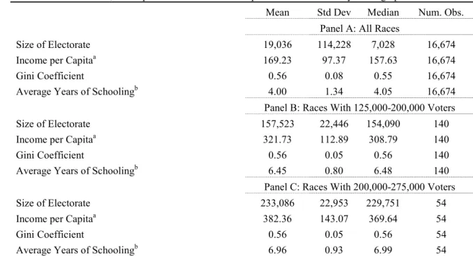
Tables 1A-1C contain some relevant descriptive statistics. In Table 1A we can see

that the vast majority of municipalities in Brazil are small: half of the 16,674 races occurred

in municipalities whose electorate was smaller than 7,066 voters. As expected, municipalities

with more than 125,000 voters are quite different from the average municipality: years of

schooling and income per capita increase with population. It is interesting to note that income

inequality within larger cities is not different from the rest of the country. Finally, there is no

substantial difference between municipalities to left and to right of the discontinuity, as

panels B and C reveal, or said in another way, the differences around 200,000 are neither

large in practice nor statistically significant. In summary, demographics suggest that

municipalities slightly below and above 200,000 are alike.

[insert Table 1 here]

The background of the first stage appears when we also look at Table 1B. The size of

electorate and the number of candidates are positively related, which is expected as the size

of the political market induces entry. The number of candidates increases considerably

around the discontinuity threshold: from an average of 4.67 in municipalities whose

electorate is between 125,000 and 200,000, to 5.45 in municipalities with electorate between

200,000 and 275,000. Same pattern arises for the median.

Following the political economy literature,19 _{we use two different measures of}

political competition: the number of effective candidates, which is the inverse of the

Herfindahl-Hirschman Index (HHI), and the percentage of votes for all candidates except the

first and second placed candidates in the first round. The HHI is the sum of squared market

shares (in this case, vote shares) and is usually normalized to be within the [0;10,000].

Finally, note the only consider races where at least three candidates ran since there is no

reason why the presence of the second round should make any difference if there are one or

two first-round candidates.

Electoral competition as measured by the number of effective candidates similarly

follows the pattern of number of candidates. We can see that the number of effective

candidates increases with electoral size. Around the discontinuity point 200,000, the number

19

of effective candidates increases from 2.65 to 2.81. The same result arises when

concentration is measured by the percentage of votes received by the 3rd placed candidate or

lower. This percentage rises from 18.35% in municipalities with electorate size between

125,000 and 200,000 to 22.41% in municipalities with electorate size between 200,000 and

275,000. Again, both are significantly higher than in the whole sample (14.71% on average).

Table 1C shows some statistics for four fiscal variables: investment as proportion of

total spending, current spending as proportion of total spending, payroll as proportion of total

spending and increase (in %) in the number of municipal public schools. We restricted our

attention to municipalities in the range 125,000-275,000 voters and divided the sample into

four groups: races where the incumbent could run for reelection, below and above the

discontinuity; and races where, given the inexistence of the reelection or the impossibility of

a reelection (given by the rule), the incumbent could not run for reelection, again below and

above the discontinuity.

Before 1997 incumbent mayors, governors and presidents could not run for

reelection. In January 1997, Congress amended the Constitution to allow reelection, with at

most two consecutive terms. Hence, while incumbent mayors could not run for reelection in

1996, all incumbents could in 2000. In our sample for 2000, 77% of the incumbents actually

ran for reelection. In 2004, only 52% of the incumbents were in their first terms, and could

run. Out of those, 91% ran for reelection.

We can see from Table 1C that for reelection races, the fiscal variables follow the

expected pattern: average investment and investment in education (number of schools) are

larger and average current and payroll spending are smaller for municipalities to the right of

the discontinuity (200,000-275,000) when compared to municipalities to left of the

discontinuity (125,000-200,000). The same pattern, however, cannot be found for

3. Some Graphical Evidence of the Regression Discontinuity Design

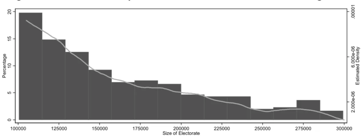
The exogeneity of the run-off is confirmed by the actual distribution of electoral size.

Figure 1 shows the histogram and kernel density estimate of the electorate size. A significant

discontinuity at 200,000 would raise the suspicion that municipalities were manipulating the

electorate size. As expected, the histogram shows that the frequency drops almost

monotonically with electorate size. The histogram shows a slight drop from bin [186,000 ;

200,000] to bin [200,000 ; 214,000], but it is not particularly pronounced compared with

other fluctuations in the figure. Still, given the drop in the histogram, we further investigate

the possibility of manipulation by estimating the density below and above the discontinuity

point 200,000, a procedure inspired in McCrary (2008).20

[insert Figure 1 here]

Figure 2A shows a small discontinuity at 200,000, already suggested by the histogram

in Figure 1. This tiny discontinuity is neither practically nor statistically significant.21 _In

Figure 2B, we repeat the procedure at 150,000. The “discontinuity” is larger now, despite the

absence of any reason for the electorate distribution to have any discrete change at 150,000.

[insert Figure 2 here]

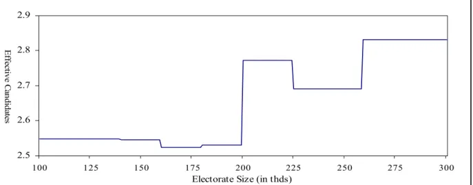
In Figure 3 we provide some preliminary graphical evidence of the behavior of

concentration around the discontinuity threshold, which shows that the first stage regression

is not weak. Imbens and Lemieux (2008) propose a histogram-type procedure. We construct

8 bins by dividing the [100,000;200,000] interval into five mutually exclusive equal-sized

sub-intervals of width 20,000, and by dividing the [200,000;300,000] interval into three

intervals: (200,000;225,000], (225,000;255,000] and (255,000;300,000]. The asymmetry is

due to the rapidly decreasing number of observations for larger electorate sizes. The larger

bin width in the (100,000,200,000] interval guarantees at least 20 observations per bin. For

20

The procedure consists of two parts. The first stage estimates the histogram in Figure 1. The second stage consists in estimating two local linear regressions, above and below the discontinuity point. The percentage of observations in each bin is treated at the dependent variable, and the midpoint of the bins as regressors. See McCrary (2008) for further details.

21

each bin, we compute the average number of effective candidates and % of votes received by

the 3rd or lower placed candidates, and attribute this number for all values in the bin width.

[insert Figure 3 here]

While in the [100,000 ; 200,000] interval, the number of effective candidates remains

roughly constant around 2.53, it jumps to 2.77 in the (200,000 ; 225,000] interval, and

fluctuates around this level over the (200,000,300,000] interval. Results are even stronger for

the % of votes received by the 3rd or lower placed candidates. Of course, these are

unconditional differences.

4. Weighted Instrumental Variables Regression

We are primarily interested in the parameter β1 given by the following equation:

FISCAL_it =β₀ +β₁E

[

]

(

)

where FISCALit is a fiscal policy outcome in municipality i at an year t prior to the election

year τ (t < τ ); POLCOMPiτ is the level of political competition in the next election that is

expected by the incumbent when making policy decisions over the administration cycle.

Political competition is measured by concentration of vote shares, and β1 is the causal effect

of the expected competition at election year τ on policy outcome variables. ELECT is the

size of electorate (number of registered voters). Fiscal policy may change systematically with

the city size, and the empirical strategy hinges on using the 200,000 rule. Thus, the inclusion

of φ(.) - a flexible function of electorate - is crucial for identifying causality. Finally,C_it is a

vector of controls such as year dummies, a polynomial of the number of candidates, and the

fragmentation in the city council.

As mentioned previously, the intensity of political competition is likely to be affected

by the quality of policies (reverse causation), so Cov

[

]

OLS estimation strategy would fail to recover the causal impact of POLCOMP on policy

outcomes. Moreover, political competition is measured with error by construction. Ideally,

political environment will be in next election. Unfortunately, that expectation is not

observable.22 _{The alternative often used in the literature on political cycles (which we}

emulate) is to use actual, realized political competition. In other words:

POLCOMP_iτ =E

[

]

where υ_it is uncorrelated with E

[

]

measurement error causes attenuation bias, which would work against finding an impact of

political competition on policy choices when OLS is used.

Therefore, we have to estimate (1) by a two-stage least squares procedure. The first

stage consists of estimating the expectation of the actual POLCOMP conditional on

DUM200, a flexible polynomial of electorate size and other controls:

[

₍

₎

]

r r

r

r r r

r

C ELECT

DUM

C DUM

ELECT POLCOMP

E

Η + +

+

= _{0 1} 200 ₁

, 200 ,

|

φ γ

γ (3)

where r is electoral race, i.e., a municipality in an election year and φ₁(.) is a flexible

polynomial of electorate of electorate that may have different functional forms above and

below the threshold point.

Note that the number of candidates increases with electoral size, and concentration

falls with the number of candidates. Thus, although descriptive statistics and some visual

analysis suggested that the concentration of voting drops around 200,000, we could not be

conclusive only with these pieces of evidence given the mechanical relationship between the

number of candidates and the effective number of candidates.23 _{Equation (3) will thus be}

useful for checking whether the pattern suggested by Table 1 survives after we control for a

polynomial of the number of candidates, a function of the electoral size and other controls.

The outcome equation (Equation 1) can be rewritten using the actual political

competition instead of the expected one. We are interested in estimation of the parameter β₁

22

It is conceivable that one could use opinion polls during the administration cycle. However, these polls are not conducted at a sufficient number of mid-sized municipalities to implement any quantitative empirical procedure.

23

FISCAL_r =β₀ +β₁POLCOMP_r +φ₂

(

)

where φ₂(.) is a flexible function of electorate size that may behave differently below and

above the threshold value.

In order to identify β₁, one may proceed in two different ways. The “conventional”

one imposes that ζ_r is uncorrelated with DUM200r (the instrumental variable), which, by its

turn, is correlated with POLCOMP given ELECT_r and C_r. A local version of it imposes that

such stochastic relationships should hold only in a neighborhood of ELECT_r= 200,000.

We follow the local identification strategy as it is more plausible to assume that any

non-controlled factor will be randomly assigned to municipalities immediately before and

after the 200,000 point. In other words, there is nothing systematic that could affect political

competition when we compare municipalities on both sides of the threshold, the only

difference being the difference in the voting rule.

Hahn, Todd and van der Klaauw (2001) have shown that local IV assumptions yield

the same identification result as imposing two continuity assumptions: Given ELECT_r and

r

C , the conditional expectation of POLCOMP and the conditional expectation of FISCAL are

continuous at the ELECT_r= 200,000. Thus, the only way FISCALr can respond to changes in

the E

[

]

andELECT_r= 200,000) is through changes from the left to right of the discontinuity. Of

course, given that we had fixed ELECT_r= 200,000, this is a counterfactual exercise that only

makes sense in a close neighborhood of the threshold.

The final identification result allows us to write β₁ actually as

(

)

(

)

r C z POLCOMP

C z FISCAL

, ,

0 0

1 _Δ

Δ =

β (5)

where z0=200,000 and

(

)

FISCAL ₀,

Δ

–E[FISCALr–φ2

(

)

and

(

)

POLCOMP ₀,

Δ

=limh↓0{E[POLCOMPr–φ1

(

)

(

)

Unless we have a large number of observations literally at the discontinuity (199,999

and 200,001, for example) to nonparametrically estimate the above four conditional

expectations, consistent estimation hinges on correctly specifying φ₁(.) and φ₂(.). We thus

proceed with estimation of β₁ on the following ways.

We start by using a simple 2SLS regression, following the equivalence result

suggested by Imbens and Lemieux (2008). They argue that (i) setting φ₁(.) and φ₂(.) to be

linear splines and (ii) discarding data points that are outside a window of size h to the left and

to the right of the discontinuity, a unweighted 2SLS will be algebraically equivalent to the

local linear Wald estimator proposed by Hahn, Todd and van der Klaauw (2001) if all four

estimates used in their formula use the same rectangular kernel and bandwidth h.

We generalize (and prove) Imbens and Lemieux (2008) result to polynomial splines

and general weighting functions. We provide in the appendix a generalizing equivalence

result for the case that kernel is not necessarily rectangular and the polynomial function may

not be linear. We thus use a weighted two-stage least squares procedure that (i) gives

weights, W, that decrease as a function of the distance to the cutoff point and (ii) controls for

polynomial splines. In fact, φ₁(.) and φ₂(.) are functions of G(k), an order k polynomial

interacted with the instrument in the following way: 24

24

G(k)=

(

)

(

)

(

)

(

)

(

)

Thus, our estimator corresponds specifically to the coefficient of POLCOMP in a

weighted IV regression using FISCAL as dependent variable, POLCOMP as the endogenous

regressor, G(k) and other elements of vector C as exogenous regressors, DUM200 as the

instrumental variable and W as the weighing function. In the appendix we present some

equivalent ways to algebraically express βˆ₁, our weighted 2SLS estimator of β₁.

5. Results

5.1. First Stage Results

In the last section we argued that consistent estimation of the structural parameter β1

involved finding exogenous variation in political competition. In section 3 we presented

some graphical evidence that this was true. We now present our first stage results.

Table 2 reports results from six regressions each one using two different measures of

political competition as dependent variable. We obtain results that are very similar, using

either the number of effective candidates or the percentage of votes of all candidates placed

third or lower.25

In all of the six regressions, the right-hand side variables are DUM200, ELECT and

its square, number of candidates, squared number of candidates, and year dummies. Column

25

(1) reports the first stage for all races, using no weights. We can see that using the whole

sample, it seems that there is nothing special with the threshold of 200,000 in terms of

inducing political competition. Even in column (2), restricting the sample to the interval

[125,000;275,000], we still get no statistical significant impact below and after the threshold,

once we control for a quadratic function of the electorate size. In all subsequent

specifications we restrict the sample to the interval [125,000;275,000].

[insert Table 2 here]

Results dramatically change when we introduce weights. We tried two different types

of weights W1 and W2, which yield similar results. Our first weighting scheme weighs

observations by the inverse of the absolute distance to the cutoff point. Specifically,

(

)

1 200

−

−

= ELECT thd

W _r . An alternative weighing scheme is a Gaussian kernel:

⎟ ⎟ ⎠ ⎞ ⎜

⎜ ⎝ ⎛

⎟ ⎠ ⎞ ⎜

⎝

⎛ −

− =

2 2

200 exp

h

thd ELECT

W r _{, where h was chosen to be 15,000. Column (3) reports}

results with W1. We can see that the effect of “crossing” the threshold is now significant and

with the correct sign: existence of a two-round system increases political competition by

decreasing the number of effective candidates and increasing the vote share of third and

lower candidates. The 200,000 rule induces a reduction up to 34% in the vote concentration

and a substantial increase (131%) in the proportion of votes given to the third and lower

placed candidates.

In column (4) we use a higher-order polynomial of electorate size and obtain similar

results in terms of statistical significance. In column (5), in addition to the specification of

column (3), we include the interaction of DUM200 with ELECT and its square.26 _This

specification (for the case of k=2) was the focus of an extensive discussion in the last section.

It is important to notice two aspects of that column. First, the coefficient of DUM200 remains

statistically significant, for both dependent variables. Second, in both models, the gain from

introducing these interaction terms seems to be relatively small, which can be seen after a

26

In column (5) the interaction is actually between DUM200 and a quadratic function of centered (at 200,000)

simple comparison between R-squared’s from column (5) and column (3). Nevertheless, we

can reject the null hypothesis that the interactions of DUM200 with ELECT and its square are

jointly insignificant.

Finally, in column (6) we test for the relevance of the instrument. We can see at

column (6) that exclusion of DUM200 from column (3) impacts negatively and soundly on

the R-squared. This constitutes piece of evidence for instrumental variable relevance.

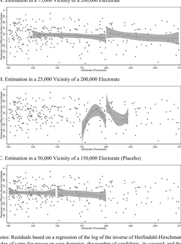
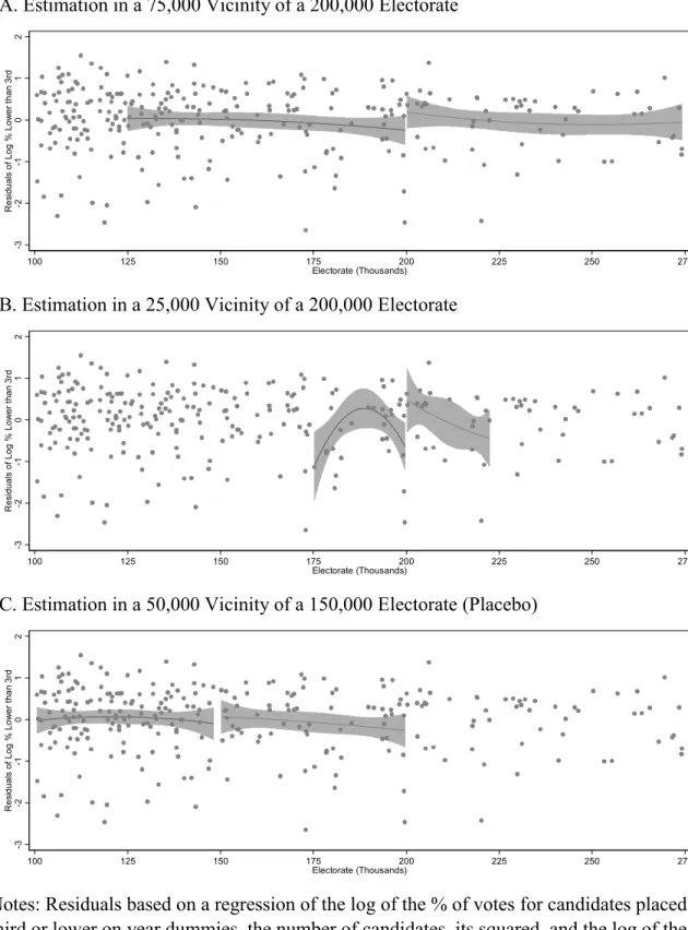
We also present more graphical evidence of a strong 1st stage. In Figure 4 panel A, we

present evidence closely related to the column (2) of Table 2. It plots the residuals of a

regression of log the number of effective candidates on covariates and fits two quadratic

functions, to left and to the right of the 200,000 threshold. We can see that although there is a

negative jump, it is not sizeable enough.

[insert Figure 4 here]

When we restrict to a much closer vicinity of the cutoff point as in panel B, the jump

is more pronounced. However, we ended up restricting ourselves to a smaller number of

observation in the interval [175,000;225,000], which clearly affects efficiency.

In Figure 5 we plot quadratic functions using, however, weights that are inversely

proportional to the distance of the cutoff point. When we introduce the weights the

discontinuity in the voting concentration is significant: municipalities with more than

200,000 voters have a more competitive electoral market than municipalities below the

200,000 threshold.

From Figure 5 we can also investigate graphically the equivalence between our

weighted method that uses quadratic (polynomial) fits for the electorate and local quadratic

(polynomial) regressions, which is shown in the Appendix. In fact, the equivalence holds

only for the values of the quadratic functions at the discontinuity. Local quadratic regressions

evaluated at a finite collection of J points of the support of the electorate would correspond to

J weighted regressions whose weights should have been centered at each of those remainder

points of the support.

We also present two robustness checks, creating a fake rule at 150,000 voters. In

Figure 4, Panel C and Figure 5, Panel B we can see that either using weights (Figure 5) or not

(Figure 4) there is no discontinuity at another value of the electorate size.

We repeat in Figures 6 and 7 the same graphical strategy, but for another measure of

political competition, log of percentage of votes of candidates placed third and lower. We

obtain the same qualitative results of Figures 4 and 5.

[insert Figure 6 here]

[insert Figure 7 here]

5.2. Second Stage Results

In the previous subsection we showed that DUM200 (a dummy for municipalities

with electorate above 200,000) increases political competition, that is, we have a strong

first-stage regression. Under the identifying assumption that DUM200 only impacts fiscal policy

through its effect on political competition, DUM200is a source of exogenous variation to

estimate β1.27 Therefore we estimate equation (4) using DUM200as an instrument.28

Three fiscal dependent variables are considered: the log of the share in total

expenditures of investment, of current spending, and of payroll expenditures. Since yearly

data is rather noisy, the dependent variables are the total share over the administration cycle.

Additionally, we also measure the impact of political competition on physical investment in

schools, measured as the change in the number of schools. For the fiscal variables, three

cycles are considered: 1993-1996, 1997-2000 and 2001-2004. Unfortunately, data on the

27

The municipalities do not bear the costs of the election, so there is no reason why crossing the 200,000 voter threshold should impact fiscal policy other than through political competition.

28

number of schools are only available for the 1997-2000 and 2001-2004 cycles. Finally,

political competition is measured by the two first-stage concentration measures previously

presented: the Herfindahl-Hirschman Index and the share of votes for the third placed

candidate or lower.

Among the controls, we include a set of year dummies, quadratic functions of the

number of candidates and of the electorate size and the Herfindahl-Hirschman Index of

concentration in the city council. Councilors are elected by direct ballot in an open-list

proportional system. The race takes place concurrently with the mayor race, and evidence

suggests that the presence of mayoral candidate may “pull” votes for her party’s councilors

(see Samuels, 2000).29 _{In this case, we might expect fragmentation in the city council to jump}

at 200,000 voters, with consequences for our identification strategy.30 _{The macro literature on}

fiscal policy and party structure suggests that fiscal adjustment is harder when the parliament

is fragmented (e.g., Milesi-Ferretti et al, 2002, and Persson and Tabellini, 2004).

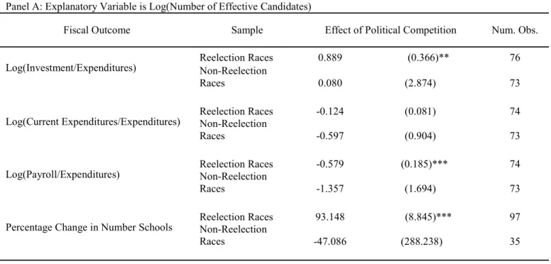
Table 3 presents the results of our weighted IV procedure. We report the coefficients

associated with the endogenous regressor for two subsamples: races in which the mayor

could run and races in which reelection was prohibited by legislation. In Panel A we use log

the number of effective candidates as endogenous regressor and in Panel B we use log of

share of votes for the third placed candidate or lower. In all procedures observations are

clustered at the state level because unobserved shocks to fiscal revenue are likely to be

correlated among cities within a certain state.31

[insert Table 3 here]

In races in which the mayor could run for reelection (panel A), a 1% increase in the

number of effective candidates causes a statistically significant increase of 0.889% of

investment as a proportion of total expenses. Results are similar when the endogenous

regressor is log of the percentage of votes received by the 3rd placed candidates or lower. A

1% increase in the proportion of votes given to the third and lower placed candidates

29

Technically, the relevant unit for the list is the coalition.

30

Indeed, it does seem that the possibility of the second round reduces the HHI at the city council by some 8%, as expected. However, the impact is not statistically significant. Results are available upon request.

31

(increase of political competition) causes a statistically significant increase of 0.157% of

investment as a proportion of total expenses. It is important to emphasize that for races in

which the incumbent mayor could not run there is no evidence of the same phenomenon,

which seems strong evidence of political competition on politicians’ behavior.

One possible concern is whether investment is the type of expenditure with most

electoral appeal. It may be that, as a response to an increase in competition, incumbents

would increase transfers, which are part of current spending. We cannot fully address this

concern because we do not have data on transfers. However, municipal transfers are very

small relative to federal transfers. We do have data on payroll spending, which does not

directly benefit most voters.32 _{When the share of payroll spending in total expenditures is}

used as the dependent variable, the results show that the reduction in current spending is due

to a reduction in personnel spending. The magnitude of the estimated impact of competition

is an order of magnitude larger for payroll than for ordinary current expenses. Again, the

results arise only for the sample of reelection races.

In races in which the mayor could run, a 1% increase in the number of effective

candidates causes a statistically significant increase of 0.579% of payroll as a proportion of

total expenses; and a 1% increase in the proportion of votes given to the third and lower

placed candidates (increase of political competition) causes a statistically significant decrease

of 0.108% of payroll as a proportion of total expenses.

Finally, we further investigate the nature of the investments made. We have data on

the number of municipal schools built and closed down during the administration cycle,

which we also use as a dependent variable in Table 3. The results suggest that increases in

political competition increase investment in education, at least as measured by physical

assets.33 _{The same pattern for reelection and non-reelection data persists: the impact of}

political competition on schools built arises only in the sample of reelection races.

32

This is certainly true for the middle-sized municipalities in our sample. In small poor cities public sector payroll can represent a substantial proportion of local income, and thus it is hard to argue that payroll spending does not have electoral appeal.

33

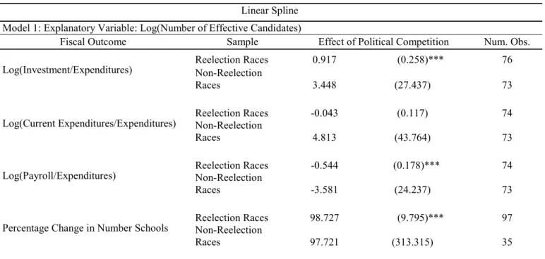
Table 4 shows estimates of the same models as in table 3, except that φ1(.) and φ2(.)

are now linear, not quadratic splines. Results are quite similar to those in table 3, which

shows their robustness to the particular form of φ1(.) and φ2(.), as long as we allow some

flexibility.

[insert Table 4 here]

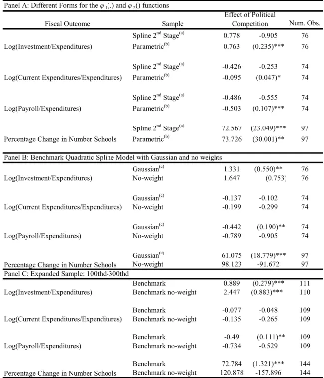
Table 5 shows several robustness tests for the quadratic model, our preferred model.

For conciseness we present only the results for the sample of reelection races.34 _{Panel A}

contains tests that concern the form of the functions φ1(.) and φ2(.). First, we include the

quadratic spline in the second stage, i.e., the function φ2(.) is a quadratic spline at 200,000

voters. Although we lose statistical significance, estimated coefficients are quite similar to

those in Table 3, showing that the exclusion of the interactions between ELECT and squared

ELECT with DUM200 in the second stage does not cause bias. Second, we run a parametric

model in which both φ1(.) and φ2(.) are a sixth degree polynomial of electorate size, but with

no splines. Results are similar to those using a quadratic function (Table 3), both in terms of

estimated coefficients and statistical significance. This confirms that estimates are not

sensitive to the particular form of φ1(.) and φ2(.), as long as we allow some flexibility.

[insert Table 5 here]

We use a weighing procedure that puts a significant weight on observations close to

200,000. The advantage of this is procedure is that we emulate as best we can the ideal

experiment of comparing cities around the discontinuity (199,999 and 200,001 voters). The

reduced number of observations and the weighting schemes that weigh very heavily

observations close to 200,000 may raise concern about outliers. For this reason we present

robustness checks in which the weights are not used, and the number of observations is

expanded to include electorate sizes between 100,000 and 300,000.35

In panel B we assess whether results are sensitive to the weighting procedure. First,

we implement a Gaussian weighting scheme, which also weighs more heavily observations

around 200,000 but less so that our scheme. Results are similar. Then, we do not weigh

34

Estimates for the subsample of non-reelection races are never significant.

35

observation at all, treating all cities in the [125,000; 275,000] interval equally. Except for

investment, no estimated coefficient is statistically significant now. However, this is driven

by reduced precision: the estimated coefficients are larger than their weighted counterparts.

Thus, weighting heavily observations around 200,000, if anything, reduces the estimated

impact of political competition on policy choices. Panel C shows that our results are not

peculiar to the [125,000; 275,000] sample. When the sample is expanded to [100,000 ;

300,000], which increases the number of observations by 30%, we get similar results.

We also present some graphical reduced form evidence. We present local regression

plots of FISCAL measures as a function of ELECT. We want to evaluate whether we can find

a discontinuity of FISCAL at 200thd. This visual evidence is called “reduced form” because

it amounts to regressing the endogenous variable on the instrument.

Figures 8 and 9 show local regression results for two different sub-samples: races in

which mayors could and races in which mayors could not run for reelection.

[insert Figure 8 here]

[insert Figure 9 here]

Inspection of Figures 8 and 9 reveals that the difference between municipalities above

and below the 200thd threshold appears only in “reelection races”. Thus, the “reduced form”

difference arises precisely where one would expect political competition to matter most.

Mayors should care more about their party’s electoral prospects if they can run for

reelection.36 _{In reelection races (Figure 8), the 200,000 threshold is associated with more}

investment, less current spending in general and payroll spending in particular, and more

schools built. For non-reelection races (Figure 9) there is no marked difference at 200,000. It

should be noted however that, for schools built, results are difficult to interpret because the

sample of non-reelection races is small. 37

36

The impossibility of running for reelection does not mean that incumbents are indifferent to election results. However, it is reasonable to assume that the incentives for pursuing better policies are substantially stronger when the incumbent has a private stake on it.

37

Our main procedure weighs observations according to the distance to 200,000. Since

the number of observation is somewhat low, there is concern that outliers may drive results.

Inspection of figures 8-9 shows that, although some observations may be outliers, they are

not close to 200,000, where results would be more sensitive to them.

6. Conclusion

This paper exploited a discontinuity in Brazilian electoral rules to show that run-off

elections are associated with more candidates and sharper political competition than

majoritarian elections. This result is in line with a large body of theoretical and empirical

evidence on electoral rules and electoral competition. A first important contribution of our

paper is to exploit a quasi-natural experiment that exogenously changes the electoral rule.

Thus, among the existing papers on this subject, our design arguably provides the cleanest

identification setup for capturing the effect of electoral rules on electoral competition.

Our most interesting result, however, is related to the effect of lower entry costs for

political competition on fiscal outcomes. In theory that effect can be ambiguous and lower

entry costs may improve or worsen fiscal policy. Also, incumbent politicians can make

policy choices that directly affect political competition, which could create a reverse

causality problem.

However, by taking advantage of the discontinuity in the electoral rule as a function

of the electorate size, we can unequivocally identify the causal effect of political competition

on fiscal outcomes. Our results suggest that lower political entry costs shift public

expenditures from current expenditures towards investment, which can be perceived as

welfare improving.

Despite the sharp identification provided by the discontinuity we explore, there are

valid concerns relating to external validity. It is likely that the net effect depends on the

particular features of the setting. For example, higher competition likely affects young and

with” than national governments. But with these caveats in mind, this paper does suggest that

lower costs of political entry in a multi-party democracy are beneficial.

References

Angrist, J. and V. Lavy, “Using Maimonides’ Rule to Estimate the Effect of Class

Size on Scholastic Achievement,” Quarterly Journal of Economics, Vol. 114, pp. 533–576,

1999.

Besley, T. and A. Case, “Incumbent Behavior: Vote-Seeking, Tax-Setting and

Yardstick Competition,” American Economic Review, Vol. 85, pp. 25-45, 1995.

Besley, T. and A. Case, “Does Electoral Accountability Affect Economic Policy

Choices? Evidence from Gubernatorial Term Limits,” Quarterly Journal of Economics, Vol.

110, pp. 769-798, 1995.

Besley, T. and A. Case, “Political Competition and Policy Choices: Evidence from

the United States,” Journal of Economic Literature, Vol. 841, pp. 7-73, 2003.

Besley, T., T. Persson and D. Sturm, “Political Competition and Economic Performance: Theory and Evidence from the United States,” NBER Working Paper Series 11484, 2005.

Black, S., “Do Better Schools Matter? Parental Valuation of Elementary Education,”

Quarterly Journal of Economics, Vol. 114, pp. 577–599, 1999.

Campante, F., D. Chor and Q. Do, “Instability and the Incentives for Corruption,” SSRN Working Paper, 2008.

Degan, A. and A. Merlo, “A Structural Model of Turnout and Voting in Multiple Elections,” PIER Working Paper 07-011, 2007.

Duverger, Maurice Political Parties, New York: Wiley, 1954.

Fan, J., Gijbels, I., Local Polynomial Modeling and its Applications, Chapman &

Hall, London, 1996.

Ferraz, C. and F. Finan, “Exposing Corrupt Politicians: The Effects of Brazil’s

Publicly Released Audits on Electoral Outcomes,” Quarterly Journal of Economics,Vol.

123, pp. 703-745, 2008.

Ferreira, Fernando and Joseph Gyourko, “Do Political Parties Matter? Evidence from

US Cities,” Forthcoming, Quarterly Journal of Economics.

Hahn, J., P. Todd and W. Van der Klaauw, “Identification and Estimation of

Treatment Effects with Regression Discontinuity Design,” Econometrica, Vol. 69, pp.

201-209, 2001.

Imbens, G. and T. Lemieux, “Regression Discontinuity Designs: a Guide to Practice,”

Jones, M. Electoral Laws and the Survival of Presidential Democracies, Notre Dame: University of Notre, 1995.

Laakso, M. and Taagepera, R. “The "Effective" Number of Parties: a Measure with Application to Western Europe,” Comparative Political Studies, Vol 12, pp. 3-28, 1979.

Lee, D., “Randomized Experiments from non-Random Selection in U.S. House

Elections,” Journal of Econometrics, Vol. 142, pp. 675-697, 2008.

Lemieux, T. and M. Milligan, “Incentive Effects of Social Assistance: a Regression

Discontinuity Approach,” Journal of Econometrics, Vol. 142, pp. 807-828, 2008.

McClintock, C., “Plurality versus Runoff Rules for the Election of the President in

Latin America: Implications for Democracy,” Annals of the Meeting of the American

Political Science Association, 2007.

McCrary, J. “Manipulation of the Running Variable in the Regression Discontinuity

Design: a Density Test,” Journal of Econometrics, Vol. 142, pp. 698-714, 2008.

Merlo, A., “Whither Political Economy? Theories, Facts and Issues,” in Advances in

Economics and Econometrics, Theory and Applications: Ninth World Congress of the Econometric Society, eds. Blundell, R., W. Newey and T. Persson, Cambridge: Cambridge University Press, 2006.

Milesi-Ferretti, R. Perotti and M. Rostagno, “Electoral Systems and Public

Spending,” Quarterly Journal of Economics, Vol. 107, pp. 609-657, 2002.

Palfrey, T. “A Mathematical Proof of Duverger’s Law,” in Models of Strategic

Choice in Politics, ed. Ordeshook, P., Ann Arbor: The University of Michigan Press, 1989.

Persson, T. and G. Tabellini, “Constitutional Rules and Fiscal Policy Outcomes,”

American Economic Review, Vol. 94, p. 25-45, 2000.

Rodgers, D. and J. Rodgers, “Political Competition and State Government Size: Do

Tighter Produce Looser Budgets?” Public Choice, Vol. 105, pp. 1-20, 2000.

Rogoff, K., “Equilibrium Political Budget Cycles,” American Economic Review, Vol.

80, pp. 21-36, 1990.

Samuels, D., “The Gubernatorial Coattails Effect: Federalism and Congressional

Elections in Brazil,” The Journal of Politics, Vol. 62, pp. 240-253, 2000.

Thistlewaite, D. and D. Campbell, “Regression-Discontinuity Analysis: An

Alternative to the Ex Post Facto Experiment,” Journal of Educational Psychology, Vol. 51,

pp. 309–317, 1960.

Van Der Klaauw, W., “Estimating the effect of financial aid offers on college

enrollment: a regression-discontinuity approach,” International Economic Review, Vol. 43,

Table 1.A, Descriptive Statistics for Municipal Election Races: City Demographics

Mean Std Dev Median Num. Obs. Panel A: All Races

Size of Electorate 19,036 114,228 7,028 16,674

Income per Capitaa 169.23 97.37 157.63 16,674

Gini Coefficient 0.56 0.08 0.55 16,674

Average Years of Schoolingb 4.00 1.34 4.05 16,674

Panel B: Races With 125,000-200,000 Voters

Size of Electorate 157,523 22,446 154,090 140

Income per Capitaa 321.73 112.89 308.79 140

Gini Coefficient 0.56 0.05 0.56 140

Average Years of Schoolingb 6.45 0.80 6.48 140

Panel C: Races With 200,000-275,000 Voters

Size of Electorate 233,086 22,953 229,751 54

Income per Capitaa 382.36 143.07 369.64 54

Gini Coefficient 0.56 0.05 0.56 54

Average Years of Schoolingb 6.96 0.93 6.99 54

Source: Tribunal Superior Eleitoral, Secretaria do Tesouro Nacional and Instituto Brasileiro de Geografia e Estatística.

a

In 2000 reais

b

Years of schooling for the population between 15 and 64 years old.

Table 1.B, Descriptive Statistics for Municipal Election Races: First Stage Variables

Mean Std Dev Median Num. Obs. Panel A: All Races

Number of Candidates 2.79 1.12 2.00 16,500

Effective Number of Candidatesa 2.51 11.83 2.40 8,144

Share of Votes of Third Placed and Lowerb 14.71 11.83 12.40 8,144

Panel B: Races With 125,000-200,000 Voters

Number of Candidates 4.67 1.42 4.00 134

Effective Number of Candidatesa 2.65 0.60 2.50 134

Share of Votes of Third Placed and Lowerb 18.35 11.85 16.66 134

Panel C: Races With 200,000-275,000 Voters

Number of Candidates 5.45 1.58 5.00 55

Effective Number of Candidatesa 2.81 0.70 2.67 55

Share of Votes of Third Placed and Lowerb 22.41 13.48 21.66 55

Source: Tribunal Superior Eleitoral, Secretaria do Tesouro Nacional and Instituto Brasileiro de Geografia e Estatística

a

The number of effective candidates is the inverse of the Herfindahl-Hirschman Index (HHI) multiplied by 10,000. Only races with more than 2 candidates included

b

Table 1.C, Descriptive Statistics for Municipal Election Races: Second Stage Variables

Mean Std Dev Median Num. Obs. Panel A: Races With 125,000-200,000 Voters,

Reelection Races

Investment as % of Total Spendingc 12.88 6.67 11.13 59

Current Spending as % of Total Spendingc 75.13 8.38 77.02 58

Payroll Spending as % of Total Spendingc 52.51 14.88 49.59 58

% Change in Number of Schools 11.37 21.72 6.87 74

Panel B: Races With 200,000-275,000 Voters, Reelection Races

Investment as % of Total Spendingc 13.01 6.64 11.11 22

Current Spending as % of Total Spendingc 74.86 9.56 77.44 21

Payroll Spending as % of Total Spendingc 50.57 16.21 46.72 21

% Change in Number of Schools 14.83 34.43 9.05 28

Panel C: Races With 125,000-200,000 Voters, Non-Reelection Races

Investment as % of Total Spendingc 17.16 6.93 17.13 52

Current Spending as % of Total Spendingc 69.76 12.04 70.06 52

Payroll Spending as % of Total Spendingc 47.73 17.38 44.07 40

% Change in Number of Schools -0.73 9.67 0.00 25

Panel D: Races With 200,000-275,000 Voters, Non-Reelection Races

Investment as % of Total Spendingc 15.50 6.53 14.84 23

Current Spending as % of Total Spendingc 71.15 9.25 73.83 23

Payroll Spending as % of Total Spendingc 53.84 13.82 50.15 23

% Change in Number of Schools 3.08 16.44 3.20 13

Source: Tribunal Superior Eleitoral, Secretaria do Tesouro Nacional, Instituto Brasileiro de Geografia e Estatística and Ministério da Educação

a

Percentage of votes received by candidates placed third or lower in the first round. Only elections with more than 2 candidates included

b

Herfindahl-Hirschman Index, the sum of the squares of the voting shares of all candidates times 10,000. Only elections with more than 2 candidates included

c

Table 2. OLS Regressions For Vote Share Concentration

All Races 125,000-275,000

125,000-275,000

125,000-275,000

125,000-275,000

125,000-275,000

Panel A: Dependent Variable: Log(Number of Effective Candidates)

(1) (2) (3)(a) (4)(b) (5)(a) (c) (6)(a)

-0.029 0.074 0.342 0.150 0.386

Dummy For 200,000 or

More Voters _{(0.033) (0.051) (0.027)*** (0.060)** (0.030)***} -

-2.16e-07 5.43e-07 5.64e-06 0.002 1.01e-05 1.21e-06 Electorate Size

(6.79e-08)*** (3.08e-06) (4.43e-06) (0.006)

(2.16e-06)*** (3.98e-06) 3.46e-14 -4.44e-12 -2.57e-11 -3.32e-08 -1.20e-10 -3.95e-12 Electorate Size Squared

(9.23e-15)*** (8.50e-12) (1.28e-11)* (8.11e-08)

(3.39e-11)*** (9.87e-12)

0.207 0.201 0.181 0.199 0.157 0.368

Number of Candidates

(0.013)*** (0.059)*** (0.080)** (0.055)*** (0.084)* (0.117)***

-0.011 -0.010 -0.011 -0.010 -0.009 -0.024

Number of Candidates

Squared _{(0.001)*** (0.005)* (0.008) (0.004)*** (0.008) (0.011)**}

Quadratic Spline No No No No Yes No

R2 0.253 0.308 0.644 0.317 0.669 0.399

Number of Observations 8092 187 187 187 187 187

Panel B: Dependent Variable: Log(100-Vote Share of Top Two Candidates)

-0.094 0.273 1.316 0.584 1.500

Dummy For 200,000 or

More Voters _{(0.205) (0.323) (0.295)*** (0.332)* (0.300)***} -

-4.17e-07 -4.61e-06 -9.29e-06 0.007 5.93e-05 -2.63e-05 Electoral Size

(2.36e-07)* (8.17e-06) (2.89e-05) (0.020)

(2.10e-05)*** (2.75e-05) 1.13e-13 2.83e-12 -2.17e-11 -1.14e-07 -7.09e-10 6.18e-11 Electoral Size Squared

(3.73e-14)*** (2.07e-11) (6.95e-11) (2.69e-07)

(2.47e-10)*** (6.86e-11)

1.222 0.960 1.487 0.952 1.372 2.206

Number of Candidates

(0.085)*** (0.218)*** (0.801)* (0.207)*** (0.791)* (0.912)**

-0.076 -0.059 -0.105 -0.059 -0.097 -0.156

Number of Candidates

Squared _{(0.008)*** (0.017)*** (0.064) (0.016)*** (0.063) (0.074)}

Quadratic Spline _{No No No No Yes No}

R2 0.137 0.305 0.617 0.313 0.635 0.475

Number of Observations 8092 187 187 187 187 187

Notes: Only races with more than 2 candidates considered. Standard errors in parenthesis. *, ** and *** indicate statistical significance at the 10%, 5% and 1% levels respectively. All regressions include year dummies and the HHI index of votes for the city council.

(a)