S
HOULD
V
OTERS BE
A
FRAID OF
H
ARD
B
UDGET
C
ONSTRAINT
L
EGISLATION
?
F
ISCAL
R
ESPONSIBILITY
L
AW IN
B
RAZILIAN
M
UNICIPALITIES
P
AULO
A
RVATE
C
ARLOS
P
EREIRA
Outubro
de 2009
T
T
e
e
x
x
t
t
o
o
s
s
p
p
a
a
r
r
a
a
D
TEXTO PARA DISCUSSÃO 232 • OUTUBRO DE 2009 • 1
Os artigos dos Textos para Discussão da Escola de Economia de São Paulo da Fundação Getulio
Vargas são de inteira responsabilidade dos autores e não refletem necessariamente a opinião da
FGV-EESP. É permitida a reprodução total ou parcial dos artigos, desde que creditada a fonte.
Escola de Economia de São Paulo da Fundação Getulio Vargas FGV-EESP
Should Voters be Afraid of Hard Budget Constraint Legislation?
Fiscal Responsibility Law in Brazilian Municipalities
♣Paulo Arvate
Visiting Professor, Department of Political Science, Michigan State University – MSU Professor, São Paulo Business and Economics School – FGV
E-mail: [email protected]
Carlos Pereira
Assistant Professor, Department of Political Science, Michigan State University – MSU Professor, São Paulo School of Economics – FGV
E-mail: [email protected]
Abstract
This manuscript demonstrates that voters have nothing to be afraid of when new hard budget constraint legislation is implemented. Our claim is that this kind of legislation reduces the asymmetry of information between voters and incumbents over the budget and, as a consequence, the latter have incentives to increase the supply of public goods. As a nationwide institutional innovation, the Fiscal Responsibility Law (FRL) is exogenous to all municipalities; therefore, there is no self-selection bias in its implementation. We show that public goods expenditure increases after the FRL. Second, this increase occurs in municipalities located in the country’s poorest region. Third, our findings can be extended to the supply of public goods because the higher the expenditure with health and education, the greater the probability of incumbents being re-elected. Finally, there exists a “de facto” higher supply of public goods in education (number of per capita classrooms) after the FRL.
Key words: Hard Budget Constraint; Institutional Shock; Fiscal Responsibility Law; Supply of Public Goods.
JEL classification: H39, H49; H75.
♣
1. Introduction
Politicians are tempted to behave opportunistically with voters under new hard budget constraint legislation (Poterba and Ruben 2001). This might be particularly true when policymakers face the situation of low tax revenue and/or several social distortions such as high social inequalities and high level of illiteracy. As such, it is expected that politicians would be biased or tempted to avoid supporting this kind of balanced budget initiative. That is, they would try to self-select to participate in this process. We claim, however, that voters have nothing to be afraid of because this threat is not credible. At the end of the day, politicians want to survive electorally and in order to do so they have to meet voters’ demands for public goods, especially when they are fiscally constrained.
Our findings counterintuitively indicate that voters in municipalities in the worst situation, located in poor regions, have access to a higher public goods expenditure and, in the case of education, there is evidence of higher supply of public goods after the implementation of the Fiscal Responsibility Law – FRL.1 We use the case of Brazil to demonstrate that the supply of public goods is higher in municipalities that are located in the country’s poorest regions, when compared to any other region, after the adoption of balance budget rules.
We argue that the implementation of the FRL produced an institutional shock that reduced the asymmetry of information between voters and incumbents.2 The FRL provided
information to voters about its fiscal result and its components related to revenue and expenditure. Within this new set of rules, the average of municipalities in our sample reduced the size of government. In opposite directions, municipalities located in poorest regions increased government size and tax revenue. Our main results show that public goods expenditure is higher in municipalities located in the poorest regions. More specifically, poor municipalities experienced a considerable increase in per capita education, health, and investment expenditures. Bear in mind that education and health are the largest per capita expenditures in Brazilian municipalities. Greater investment means a higher supply of public goods in the future. Our tests also demonstrate that the difference in public goods expenditure (particularly with education) between municipalities located in poorest and richest regions was reduced after the implementation of the FRL. We imposed robustness checks to verify whether public goods expenditure can be in fact interpreted as “public good.” We have two telltale signs that it is the case: mayors who increase expenditures with public policies for
1
Public goods expenditure is used as a “proxy” for public goods where there is not directly available information on the supply of public goods. See Persson and Tabellini (1998).
2 See Persson and Tabellini (2000) for problems with asymmetry of information between incumbents and voters
health and education heighten their probability of electoral success. In other words, voters reward incumbents if they receive more public goods through more expenditure. Moreover, the number of per capita classrooms rose in municipalities located in the country’s poorest regions.
In the United States, there exists greater independence to approve balanced budget legislation at the municipal level (where supposedly selection bias seems to occur more often), as well as an organized market for subnational public debt. In contrast, since 1997 Brazil has not had an organized market for new subnational debts.3 However, a tough federal
legislation was passed in the year 2000: the FRL. This law, which was applicable to all municipalities regardless of their prior economic conditions, goes against fiscal irresponsibility.4 Differently from Poterba and Ruben (2001),5
however, our analysis is free from endogeneity because the FRL was an exogenous imposition to all municipalities; that is, nobody could self-select to participate or avoid participating given the new constraints generated by the law. Beyond the above-mentioned characteristic of a centralized set of laws imposed top-down on all municipalities, Brazil is an important case to study considering that there is enough variation of per capita income across its regions (see Table 1).
[Table 1 about here]
In addition, voting is compulsory in Brazil for all individuals aged between 18 and 65 years. This institutional feature leads to a large share of individuals that receive public goods for participating in the electoral process. In countries without this formal obligation, politicians might not take into account the preferences of voters who decide not to play the democratic game.
3 In 1996, an investigatory committee (Inquiry Parliamentary Committee) in the Senate found a series of frauds
and irregularities on the process of issuing new public debts and negotiation of public debts by states and municipalities. At that time, given the excessive number of government bonds in the market, the Senate approved a bill of new bonds to be used only to finance the payment of legal debts of states or municipalities. Therefore, some states and municipalities created fictitious judicial debts in order to obtain authorization to issue new debts. Furthermore, these fraudulent issues were associated with negotiation schemes in the secondary debt market, which were equally fraudulent and generated a loss for the public treasury and profits for some brokers and banks. In 1998, in reaction to this crisis, the Senate approved Resolution 78 in which the “new public securities” were banned until 2010. See Arvate, Biderman and Mendes (2008) for more details.
4 See other Latin American experiences in Lora (2006).
5
We used three econometric techniques to test our main hypotheses. First, the Prais-Winsten model with estimation of panel-corrected standard errors (Beck and Katz 1995, 1996) was used to capture the effect of the FRL on public goods expenditure (education, health, public order and safety, housing, transportation, and investments) of municipalities and on the supply of public goods (number of teachers, number of classrooms and enrollments). Second, we also applied the Oaxaca and Ransom’s (1994) decomposition to capture the possible effect of the FRL on the reduction of differences in social expenditures between municipalities in the country’s richest and poorest regions. Finally, we used the dProbit model (marginal effects) to investigate if an increase in health and education expenditures raises the probability of re-election of an incumbent mayor. We worked with a fairly large sample size, about 5,560 municipalities in two consecutive administrations (1997-2000 and 2001-2004). This strategy allows us to comparatively investigate two distinct periods: before and after the restrictions imposed by the FRL.
The paper is organized as follows: Section 2 discusses the literature that specifically deals with the effect of budgetary rules on fiscal performance. Section 3 discusses the main components of the FRL, emphasizing the importance of budget rules to fiscal results and showing the effects of FRL on municipalities located in the poorest regions through three main fiscal variables: per capita current expenditure (which usually measures government size); per capita transfers received from federal and state governments; and per capita tax revenue. Section 4 presents a formal model of the FRL as an institutional shock, which provided incentives for incumbent politicians to increase the supply of public goods. Section 5 presents the empirical analysis, describing our data and empirical strategies, discusses the results, and performs some robustness tests. Finally, Section 6 concludes by highlighting the main results.
2. Literature on budget rules and fiscal results
governments (Poterba, 1994) and that power dispersion increases the chances of fiscal profligacy. In this respect, Roubini and Sachs (1989: 905), for instance, argue
“when power is dispersed, either across branches of the government (as in the US), or across many political parties through the alteration of political control over time, the likelihood of inefficient budgetary policy is heightened. Thus they find that the size and persistence of budget deficits in industrial countries in the past decade is greatest where there have been divided government (e.g. multi-party coalitions rather than majority-party government).”
Other scholars argue that expenditures grow as the number of legislators and political parties increases, and that the budget approved by a coalition is larger than the expected budget supported by a single-party majority (Weingast 1979; Shepsle, Weingast and Christopher 1981). In multi-party legislatures, as the effective number of parties increases, coalitions become unstable and, because of the norm of universalism, the size of the budget grows (Scartascine and Crain, 2001). Electoral systems with proportional representation combined with large districts are more likely to produce weaker governments than plurality rule systems (Stein, Talvi, and Grisanti, 1998). This position is shared by Hallerberg and Marier (2004:572), who point out
“the level of the Common Pool Resource problem in the legislature depends upon the type of electoral system. If states have open list proportional representation systems, then increases in district magnitude increase the problem, while closed lists increases in district magnitude decrease the problem.”
Alesina and Rosenthal (1995) also claim that coalition governments face greater difficulties in implementing fiscal adjustments, as well as in responding to budget unbalance than unitary governments.
Several case studies on Brazil have led to similar findings. For example, Amorim Neto and Santos (2001) argue that broad and low-cohesive coalition governments should be associated with larger deficits. Thus, the greater the size of the presidential party within Congress, the smaller the side payments needed to build legislative majorities. According to Ames (2001), given the Brazilian federal structure and its electoral system (open list PR), the president can rarely avoid paying a high price, in pork and patronage, for legislative support. Finally, the political use of public resources in the form of patronage, clientelism, and patrimonialism, according to Mainwaring (1999), not only produces high costs but clearly impedes the addressing of popular preferences and collective solutions in Brazilian politics.
whether there are any ex-post veto or control are the key elements that force the decision makers (especially in Congress) to take into account “the true benefits and costs of increased spending and taxation” (von Hagen 1992; Alesina, Hausmann, Homes, and Stein 1995). The idea is that delegating authority to a fiscal entrepreneur (i.e. a strong Ministry of Finance in the Executive) increases the chances of cooperation. To be effective, this entrepreneur must have the ability to monitor the others, possess selective incentives that can be used to punish defectors and/or reward those who cooperate, and have the motivation to bear the costs of monitoring himself.
Acosta and Coppedge (2001:2), in a more extensive study on Latin American countries, claim that presidents’ partisan powers have a direct and powerful effect on spending and only an indirect effect on deficits per se. That is,
“Latin American Presidents who wished to restrain spending in the 1980s and 1990s achieved this goal to the extent that they could depend on extensive, disciplined support in Congress. However, these same institutions also helped other presidents accelerate spending if that was their goal.”
Hallerberg and Von Hagen (1997:5) propose that:
“these two literatures complement one another. Electoral institutions matter because they restrict the type of budgetary institution which a state has at its disposal at the governmental phase. A strong finance minister is feasible in states where one-party governments are the norm, and such states usually have plurality electoral systems. In multi-party governments, which are common in states with proportional representation, the coalition members are not willing to delegate to one actor the ability to monitor and punish the others. Negotiated targets provide an alternative in multi-party governments. They will be credible, however, only if all the parties can monitor and punish each other. Since parties often lack the ability to provide one or the other of these functions, targets are harder to maintain successfully than strong finance minister.”
If one just takes into account the electoral dimension described above one would expect all these elements together to generate, if not an ungovernable democracy, at least a very expensive one. Actually, since the Real plan in 1994 (which decreased the capacity of federal states to interfere in the macroeconomic stability) and especially after the introduction of the Fiscal Responsibility Law in 2000, the government has had qualified success in fiscal policy and inflation control.6 On the other hand, it would be mistaken to disregard that Brazilian electoral rule, federalism, and other decentralized institutional features are more prone to larger deficits. One of the main challenges is to analyze the combination of these
6
institutional incentives in order to better understand how contradictory incentives can provide equilibrium in the budgetary game.
3. Fiscal Responsibility Law
The Fiscal Responsibility Law – FRL (Supplementary Law number 101/2000) establishes the norms for public finance by imposing constraints upon fiscal management. The FRL contains instruments that permit risk avoidance and corrections of mismanagement that affect public accounts. These instruments are based on planning, control, transparency and accountability.7 The FRL specifies in great detail the fiscal rules governing public sector
indebtedness, credit operations, and public account reporting. The Law reinforces that the federal government is prohibited from financing subnational governments, therefore eliminating the possibility of bailouts as well as any changes in the financial clauses of the existing debt-restructuring agreement. The FRL imposes debt ceilings for each level of government on existing debt. Any excess to the limits is to be eliminated within one year, otherwise new financing and voluntary transfers from the central government are prohibited. Other sanctions include withholding federal transfers by the federal government, denial of credit guarantees and banning of new debt.8 In addition, the FRL contains a golden rule
provision for capital spending (i.e. annual credit disbursement cannot exceed capital spending). The FRL also grants constitutional status to a number of existing rules and introduces new ones. These include the following a) personnel expenditures (including pensions), capped at 60% for subnational governments; b) new, recurrent expenditure commitments requiring specification of their full funding for the year in which they become effective and for two consecutive years; c) prohibition of spending commitments that exceed one budgetary period during the last year of tenure of executives at any level of government d) tax and fiscal exemptions and abatements have to be specified in the budget along with the instruments to offset their impact on the budget for two consecutive years; and e) public financial institutions at all levels of government are not allowed to lend to their main shareholders. It would be misleading to conclude that, because of the impressive fiscal costs to the central government, the initiatives are in the interest of subnational governments. Furthermore, the fact that most of the fiscal adjustment was generated by raising tax revenue rather than by significantly cutting down on expenditure does not mean that there has not
7 More details on the FRL can be seen on the website of the Brazilian Ministry of Planning
(http://www.planejamento.gov.br/arquivos_down/lrf/integra_lei/lei_101_ingles.PDF).
8 In order to guarantee transparency in the implementation of the rules, a list of subnational governments that
been radical change in the intergovernmental balance of power. The states had to privatize or close their banks; embark on a program of fiscal modernization; reduce the relative importance of payroll (for which governors were required at least not to hire more personnel); sell enterprises; as well as to adapt their pension regimes to the federal rules (in addition to being prohibited from creating new pension institutions or legislating in this area). In sum, the states and municipalities lost significant degrees of autonomy.
As mentioned before, the implementation of the FRL was not expected by municipalities and, as a consequence, produced a shock on the political system. As a nationwide institutional innovation, the FRL is exogenous to all municipalities; therefore, there is no self-selection bias in its implementation. We decided to test the effect of the FRL on three important public accounts: government size (current expenditure), transfers, and tax revenue. Table 2 demonstrates the effect of the FRL on the three fiscal variables and the effect of the interaction between the FRL and a dummy variable, with the value of 1 for the municipalities in the poorest regions and zero, otherwise.9
[Table 2 about here]
The first columns of each variable show the effect of FRL and the effect of municipalities located in the poorest regions. The second columns add the interaction term (FRL*POOR), showing whether the effect on municipalities located in the poorest regions was altered after the implementation of the FRL. As we can see in Table 2, the FRL reduces government size to the average of municipalities, but not in municipalities located in the poorest regions (considering the sum of coefficients: negative 14.02 plus 15.56 equal to 1.54). The reduction of per capita government size was about 14.02 for the average of municipalities, but increased 1.54 in the poorest regions. Therefore, the per capita government size located in the poorest regions is 1.54 reais higher than the average of municipalities. When we consider the interaction term (second column), the actual effect of the FRL on the increase of government size in the municipalities located in the poorest regions was higher: 9.54 (negative 19.85 plus 29.39 equal to 9.54).
Looking at the sources of financing (transfers and tax revenue), the FRL increases the per capita transfers to the average of municipalities and this value are always higher in municipalities in the poorest regions (considering the sum of coefficients: 130.44 plus 28.93 equal to 159.37). The non-significance of the interaction term shows that this effect was
9 The same empirical strategy described in Section 5 was used here (Prais-Winsten model with estimation of
absent in municipalities in the poorest regions. In other words, the FRL increases the per capita transfers, but not to those municipalities located in the poorest regions.
Finally, the FRL did not cause an increase in per capita tax revenue to the average of municipalities; however, it slightly increased the per capita tax revenue to municipalities located in the poorest regions (9.54). This effect was relevant after the implementation of the FRL (10.76). In summary, on the one hand, the effect of the FRL to the average of municipalities led to the reduction in government size, increased transfers, and had no effect on tax revenue. On the other hand, the FRL increased government size, had no effect on transfers, and increased tax revenue in municipalities located in the poorest regions. That is, these results indicate that higher per capita government size in municipalities located in the poorest regions was financed with the share of per capita tax revenue. Moreover, the FRL provided important consequences for the electorate working as an institutional shock it reduced the asymmetry of information between incumbents and voters with respect to budget constraints. That is, it reduced the ability of local politicians to self-appropriate a larger share of public resources. In order to electorally survive in this constrained environment, we claim that politicians had no alternative other than to increase the supply of public goods.
4. Institutional Shock and supply of public goods
The main objective of this model is to demonstrate that an institutional shock may provide incentives for politicians to increase the supply of public goods.10 Assume that the median voter has preferences over private consumption cmand over the per capita provision of public goods g, that is
g c U
WM = ( M)+ [1]
where U(cM) is strictly increasing and strictly concave. The consumption of a median voter is equal to
M M
y
c =(1−τ) [2]
where 0≤τ ≤1 is the tax rate on income and yMcorresponds to the median income. The government’s budget constraint is
m y r
g+ (θ)=τ [3]
where r(θ) represents rents that benefit politicians, but provides no gain for voters. The ability of politicians to extract these rents depends on the quality of institutions (rule of law,
10
checks and balances, FRL, etc.), as measured by θ. We assume that r'(θ)<0, that is, better institutions reduce the amount of rents. Intuitively, better institutions can reduce asymmetries of information between voters and incumbent politicians with respect to the budget and, as a consequence, make it more difficult for politicians to withdraw rents without being accountable.
The institution variable has two components, given by:
1 − + = t t
t μ μ
θ [4]
where μt is a random variable with uniform distribution on ⎥ ⎦ ⎤ ⎢ ⎣ ⎡ − + ξ ξ 2 1 1 , 2 1
1 . Thus, its
expected value is 1, and its density isξ, and it is serially uncorrelated. We assume that institutions tend to change slowly over time because they work as endowments of a political system. It is plausible to infer that if institutions change today, they would retain some components of yesterday’s institutions (μt−1). As we said before, the FRL was a random
shock to all Brazilian municipalities.
The objective of incumbent politicians is to maximize the utility of the median voter. In order to solve this problem, we can rewrite WMas
[5]
The first-order condition is
[6]
Consider two electoral periods, say t and t+1, and assume that the FRL is implemented at the beginning of period t+1. As a result of this implementation, there is an increase in θ, hence a reduction in r(θ). This implies that
0 ) ´( 1
1 1
1 =− >
+ + + + t t t t r d dg θ
θ [7]
and
0
1 1
1
1 = > + + + + t t t M t d dg d dW θ θ [8] g r g y U
WM = ( M− − (θ))+
1 )) ( (
' y −g−r θ =
Thus, an improvement in the quality of institutions induced by the implementation of the FRL leads to an increase in the provision of public goods and, as a consequence, to an increase in the utility of the median voter.
5. Empirical Analysis
5.1. Data
Brazil has approximately 5,560 municipalities. It is important to point out that, from 1991 to 2000, the number of Brazilian municipalities grew considerably (almost 1,000 new municipalities). Thus, to prevent an inconsistent intertemporal analysis, the Brazilian Institute of Geography and Statistics (IBGE) aggregated information according to minimum comparable areas (MCA).11
Five “traditional variables” measure public goods expenditure: education, health, transportation, public order and safety and housing. In addition, we also included a variable for investment as an alternative of public good because it can represent a policymaker’s offer to provide more public goods in the future.
In order to deal with specific characteristics of municipalities, we included the following control variables in the model, at the municipal level: per capita intergovernmental grants or transfers received from both state and federal government; per capita income; number of houses with sewage treatment; total population; HDI index; Gini coefficient; the (Ln) human capital; the percentage of houses with garbage collection; percentage of individuals under 14 years old living below the poverty line; and percentage of rural population.
We control for the political effect of the permanence of the same ideological preference measured by the political party of the incumbent mayor on the choice of public goods. As left-wing governments tend to have higher social expenditures than other governments, we included a dummy variable with value one if the political party of the incumbent mayor is located in the left-wing ideological spectrum in two electoral periods, and zero, otherwise.12
Finally, we also control for voters’ characteristics in each municipality: the percentage of households with TV set and the illiteracy rate. As voting is compulsory in Brazil for
11 Minimum comparable areas (MCA) consist of geographical areas defined by the Brazilian Institute of
Geography and Statistics (IBGE) that are not subject to changes in the number of municipalities. They consist of municipalities and have constant codes over time. Consequently, even if municipalities split up or merge, they will remain in the same MCA.
12
individuals aged 18-65 years, a higher illiteracy rate (median of 0.36 to 1991 and 0.26 to 2000) may suggest a less informed voter in Brazil. For this reason, we incorporate the percentage of households with electrical power and TV set (median of 0.49 of households had TV sets in 1991 and 0.75 in 2000) as a political control. That influences the means through which information reaches voters.
The fiscal variables were built considering the average of two terms: one before the FRL (1997- 2000) and one afterwards (2001-2004). As all variables are in per capita terms, we used the 1996 population Census with regard to the variables of the 1997-2000’s term and the 2000 Census with regard to the variables of the 2001-2004’s term. The socioeconomic variables such as sewage, garbage collection, HDI, Gini coefficient, and number of individuals (under 14 years of age) below the poverty line, were built using the 1991 Census for the 1997-2000’s term and with the 2000 Census for the 2001-2004’s term. See the Appendix for the precise definition of variables used in the estimations, their sources, and descriptive statistics.
5.2. Empirical Strategies
5.2.1. Effect of Fiscal Responsibility Law on public goods expenditure
In order to capture the differentiated effect of the FRL on public goods expenditure in municipalities located in the poorest regions, we used Prais-Winsten model with panel-corrected standard errors.
The main equation is:
[9]
where i (I = 1,…., n)is the number of municipalities in the sample; t (t = 1, 2) is the number of electoral periods used (before and after the FRL); y represents public goods expenditure;
FRL t is a dummy variable which represents the implementation of the FRL (with the value
equal to one after the FRL and zero, otherwise); POORi is a dummy variable with the value
of 1 for municipalities in the poorest regions – northeast – and zero, otherwise); FRL t * POOR i is an interaction term that captures the differentiated effect of FRL on public goods
expenditure in municipalities located in the poorest regions; x’ represents the control variables; εi,t is a normally distributed stochastic component.
Although Hausmann’s test suggests that a random effect panel could cause consistent problems to our estimators, we did not apply fixed effects because they were collinear with the POOR dummy. Thus, the dummy that represents municipalities located in the poorest
t i l
t i i t
i t
t
i FRL POOR FRL POOR x
regions substitutes the fixed effect. Robust standard errors were calculated to correct for the heteroskedasticity of residuals suggested by a modified Wald test.
Like Besley, Persson, and Sturm (2005), who used a change of law as instrumental variable (IV) of political competition to investigate its effect on fiscal variables, we assume exogeneity in the causal relationship between the FRL and the fiscal variables. This decision was based on the fact that the Congress decided for the institutional change of the FRL in all municipalities simultaneously. We also assume exogeneity in the causal relationship between the municipalities located in the poorest regions (POOR) and the fiscal variables by way of two further arguments. First, a municipality cannot choose to be located in or out of the poorest region. Second, the share of per capita income of any municipality located in the poorest region is too small in order to be able to change the per capita income in the region as a whole.
5.2.2. Difference in public goods expenditure between the richest and the poorest regions
We applied the Oaxaca and Ransom’s (1994) decomposition to explain the differences in public goods expenditure in municipalities located in the country’s poorest and richest regions before and after the implementation of the FRL. The difference was decomposed into two parts: first, group differences explained by observable characteristics that determine public goods expenditure; second, group differences explained by unobservable characteristics (endowment) that determine public goods expenditure. For instance, transfers, voters’ characteristics, and the Gini coefficient are observable characteristics that explained the first differences in public goods expenditure; but there are characteristics that are not observable: another specific endowment of the municipality that is located in the poorest region.13
We assume that the difference in public goods expenditure in each group of municipalities located in the richest and poorest regions can be explained by the following equations:
i rr rr l
i rr i
rr
x
y
,=
,β
+
ε
,Δ
andΔ
y
pr,j=
x
prl ,jβ
pr+
ε
pr,j [10]where rr is the group of municipalities located in the richest region; pr is the group of municipalities located in the poorest region; i (i=1,….,n) is the municipality in the richest
13 Yun (2006) used this methodology to verify unexplained wage differences between industries. O'Donnell, van
region; j (j=1,…..,z) is the municipality in the poorest region; Δy is the difference in average public goods expenditure between two local administrations before and after the implementation of the FRL (1996-2000 and 2001-2004) in each municipality located in different regions; x’ are observable variables which explain this difference; and ε is a normally distributed stochastic component.
Using each of the differences separately in the public goods expenditure in each group of municipalities, we can show the development of differences between the two regions by:
(
)
(
)
pr jl j pr i rr l i rr j pr i
rr y x x
y , − Ε Δ , = , β , − , β ,
Δ
Ε [11]
Assuming that
β
∗=
D
β
rr,i−
(
I
−
D
)
β
pr,jwhere I is the identity matrix and D is a weight matrix. It follows that we assume three different weights: zero, half and one.
After algebraic manipulations, we have:
(
)
(
)
(
)
(
)
(
)
(
rr j pr j)
l prj i rr prj i rr l j pr l j rr j pr i rr D I D x x x D I Dx y y , , , , , , , , ) ( ) ( β β β β − − − + + − − − = Δ Ε − Δ Ε [12]
We used ordinary least squares (OLS) to estimate equation [12] because it is a linear function. The first term of the equation shows the development of differences attributable to unexplained variables. The second term shows the development of differences attributable to explained variables. We opted for using the control variables (socioeconomic variables) only with data from the 2000 Census in this specific situation.
5.3. Results
Table 3 shows the effect of the FRL on public goods expenditure in municipalities located in the poorest region:
[Table 3 about here]
(4.43). However, after the implementation of the FRL (second column), the expenditure with education was remarkably higher in municipalities located in the poorest region (29.14).This result suggests that, in addition to balancing the budget, the FRL had the effect of relocation of the municipal budget expenditures toward social policies.
As opposed to its effect on per capita education, the FRL had a positive effect on the per capita expenditure in health in the average of municipalities. Nevertheless, when we test with the interaction term (second column), the supply of health policies in municipalities located in the poorest region was higher after the implementation of the FRL (13.02 minus 8.08 plus 11.05 equal to 15.05). It is interesting to note that municipalities located in the poorest region spent less than the average of municipalities before the implementation of the FRL.
The result for the per capita transportation expenditure is independent from the FRL. Put differently, expenditures with transportation in municipalities located in the poorest region are lower than the average of municipalities. The per capita expenditure with public order and safety had a positive and statistically significant effect after the implementation of the FRL. Specifically, this type of expenditure was higher (0.78) in municipalities in the poorest region.
The future supply of public goods, captured by per capita investment, shows an interesting result. The FRL was very important to municipalities in the poorest region because it seems to change a negative tendency of investments in poor cities. While in the average of municipalities the trend is to reduce per capita investment, in municipalities located in the poorest region, the trend is the opposite; that is, this kind of expenditure increased after the implementation of the FRL (4.93).
Finally, the per capita housing expenditure was reduced for the average of municipalities after the FRL, but not in municipalities in the poorest region. These municipalities increased their per capita housing expenditure by more than 7.61 when compared to the average of municipalities after the FRL.
In general, the FRL increased public goods expenditure for municipalities in the poorest region. This conclusion is based mainly on the most important per capita expenditures of all municipalities; that is, with education and health (the average of per capita expenditures with both was 158.94 reais in 1991 and 100.60 reais in 2000). The future seems to have a bright outlook considering per capita investment.
benchmark before and after the implementation of the FRL. As we mentioned before, we used the Oaxaca and Ransom’s (1994) decomposition:
[Table 4 about here]
First, it is interesting to note that the difference in public goods expenditure before and after the implementation of the FRL between municipalities located in the richest and in the poorest regions was explained by unobservable characteristics only (endowment). At no time were traditional factors statistically significant. This result suggests that the implementation of the FRL changed some unobservable characteristic within municipalities located in the poorest region. It is plausible to attribute that this was a consequence of the institutional shock originated by the FRL, which reallocated public resources and generated an increase in public goods expenditure.
The most important result is related to expenditures with education. The coefficients of unexplained variables are statistically significant for all weight matrices (zero, half and one). The difference in expenditures with education in municipalities located in the poorest region was reduced in relation to the richest region. The supply of health and transportation presented statistically significant unexplained variables when the weight matrix was equal to 1 only. It suggests a less robust result when compared to that of education.
5.3. 1. Robustness
As it is plausible to infer that public expenditure may not necessarily mean delivering public goods, we have decided to explore robustness exercises in two ways. First, public expenditures with health and education generate electoral returns. Second, we tested the effect of the FRL on the per capita supply of three specific educational policies: number of elementary teachers, number of classrooms, and number of enrollments. In other words, we investigated if the public expenditure in fact corresponds to “public goods” by looking at specific educational policies.
tested if the party of the incumbent mayor was reelected, using a dprobit model (considering marginal effects),14 as a function of expenditures with health and education (See Table 5).15
[Table 5 about here]
Results show that, although politicians have access to a smaller amount of rents after the FRL, they are electorally rewarded by voters by providing higher public goods expenditure, regardless of how poor the municipality is. In other words, increasing education expenditure enhances the probability of reelection of the incumbent mayor’s political party. The same result occurs when mayors increase health expenditure (both during the first three years of the incumbent’s term and in the electoral year).
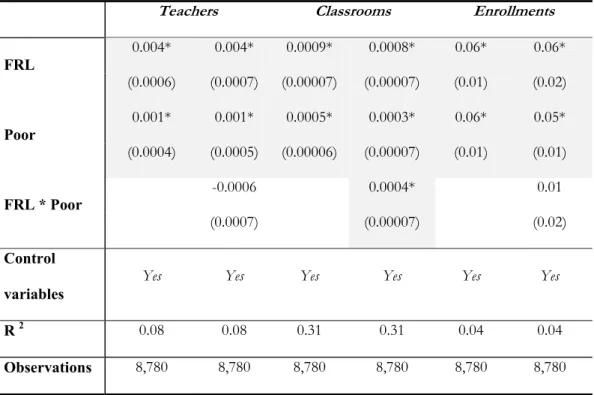
In the second robustness exercise, we gathered data concerning three variables on public education: teachers, classrooms, and students’ enrollments. Table 6 presents the results of this investigation using the same technique (panel) employed previously.16
[Table 6 about here]
Results show that the FRL increases the per capita number of teachers, classrooms, and students’ enrollments in the average of municipalities. Moreover, it is also important to observe that after the implementation of the FRL, the per capita number of classrooms increased in municipalities located in the poorest region.
6. Conclusion
The main purpose of this article is to show that voters have nothing to be afraid of when new hard budget constraint legislation is enacted. Our basic claim is that this kind of legislation reduces the asymmetry of information between voters and incumbents with respect to budget constraints and, as a consequence, increases the supply of public goods. That is, it reduces the capacity of local politicians to self-appropriate a larger share of public resources. In order to electorally survive in this constrained environment, we claim that politicians have no alternative other than to increase the supply of public goods.
Politicians can opportunistically try to argue that this process would be inadequate and engage in a process of self-selection against this kind of law (Poterba and Rueben, 1997).
14
See Wooldridge (2001) about the Probit model.
15 The note in Table 5 indicates which variables were used as control. In order to observe electoral success, we
used data from the period after the FRL (2001-2004). As we have shown that public expenditure increases, we need to investigate if this increase leads to electoral returns to the incumbent. We also added other important political control variables: mayor’s party electoral support, if the mayor’s party is the same as the governor’s, and if the mayor’s party is the same as the president’s. See the definition and descriptive statistics in the Appendix.
16
It might be particularly true in the poorest regions, where there exist fewer economic resources, larger social inequality, and a constant risk of bailing out. However, the institutional shock caused by the FRL on all Brazilian municipalities permitted us to investigate whether the supply of public goods increased without the risk of endogeneity. Our investigation provides implications for the literature in at least four important aspects. First, the implementation of the FRL was exogenous to all municipalities. Thus, it avoided the problem of self-selection bias by incumbent politicians. Second, independently from the choice of adjustment, we demonstrate that public goods expenditure increases after the implementation of the FRL. Third, the size of government and tax revenue increased simultaneously in the municipalities located in the country’s poorest region. As a consequence of the reduction in information asymmetry between voters and incumbents, politicians increased the supply of public goods in order to survive electorally. Fourth, by using Oaxaca and Ransom’s (1994) decomposition we demonstrated that the differences in public goods expenditure decreased between municipalities located in the country’s poorest and richest regions before and after the implementation of the FRL.
References
Acosta, Andrés M. and Michael Coppedge. 2001. “Political Determinants of Fiscal Discipline in Latin America, 1979-1998”. Working paper presented at the International Congress of the LASA, Washington, DC.
Alesina, A., Ricardo Hausmann, Rudolf Hommes, and Eduardo Stein. 1999. “Budget Institutions and Fiscal Performance in Latin America”. Journal of Development Economics, 59: 253-273.
Alesina, Alberto and Howard Rosenthal.1995. Partisan Politics, Divided Government, and the Economy. Cambridge: Cambridge University Press.
Ames, Barry. 2001. The Deadlock of Democracy in Brazil. Ann Arbor: University of Michigan Press.
Amorim Neto, Octavio and Fabiano Santos. 2001. “A Conexão Presidencial: Frações Pró e Antigoverno e Disciplina Partidária no Brasil.” Dados 44 (2): 291-321.
Arvate, Paulo R., Ciro Biderman, and Marcos Mendes. 2008 “Sub-national loan authorization in Brazil: is there a room for opportunistic political behavior?” Forthcoming, Dados.
Beck, Nathaniel and Jonathan N. Katz. 1995. “What To Do (and Not To Do) with Time- Series–Cross-Section Data in Comparative Politics” American Political Science Review 89: 634–647.
Beck, Nathaniel and Jonathan N. Katz. 1996. “Nuisance vs. Substance: Specifying and Estimating Time-Series-Cross-Section Models” Political Analysis 6: 1–36.
Besley. Timothy, Torsten Persson, and Daniel Sturm. 2005. “Political Competition and Economic Performance: Theory and Evidence from the United States” NBER Working Paper Series, 11484.
Hallerbergh, Mark and Patrik Marier. 2004 “Executive Authority, the Personal Vote, and Budget Discipline in Latin American and Caribbean Countries.” American Journal of Political Science, 48 (3): 571-87.
Hallerberg, Mark and Jurgen Von Hagen. 1997. “Electoral Institutions, Cabinet Negotiations, and Budget Deficits in the European Union” NBER Working Papers Series, 6341. Lora, Eduardo, ed. 2006. State of State Reform. Stanford University Press.
Oaxaca, Ronald L. and Michael R. Ransom. 1994. “On discrimination and the decomposition of wage differentials” Journal of Econometrics, 61: 5-21.
O'Donnell, Owen, Eddy van Doorslaer, and Adam Wagstaff O’Donnell. 2006. “Decomposition of Inequalities in Health and Health Care” In Elgar Companion to Health Economics, ed. Andrew M. Jones. Chichester, England: Edward Elgar.
Persson, Torsten and Guido Tabellini. 1998. “The size and scope of government: comparative politics with rational politicians.” NBER Working Papers Series, 6848.
Persson, Torsten and Guido Tabellini. 2000. Political Economy. The MIT Press, Cambridge, USA.
Poterba, James M. and Kim S. Rueben. 2001. “Fiscal rules, State Budget rules, and tax-exempt bond yields” Journal of Urban Economics, 50 (3): 537-562
Poterba, James. 1994. “State Response to Fiscal Crises: The Effects of Budgetary Institutions and Politics” Journal of Political Economy 102(4): 799-821.
Roubini, Nouriel and Jeffrey Sachs. 1989. “Political and Economic Determinants of Budget Deficits in Industrial Countries” European Economic Review 33: 9.3-938.
Scartascini, Carlos G. and W. Mark Crain. 2001. “The Size and Composition of Government Spending in Multi-Party Systems” Working paper presented at the Public Choice Society Conference, San Antonio – Texas.
Stein, Ernesto, Ernesto Talvi, and Alejandro Grisanti.1998. “Institutional Arrangements and Fiscal Performance: The Latin America Experience” NBER Working Papers Series,
6358.
Von Hagen, Jurgen. 1992. “Budgeting Procedures and Fiscal Performance in the European Communities” Economic Papers, 96.
Weingast, Barry. 1979. “A Rational Choice Perspective on Congressional Norms” American Journal of Political Science 23 (2): 245-262.
Weingast, Barry W., Kenneth Shepsle, and Johnsen Christopher. 1981. “The Political Economy of Benefits and Costs: A Neoclassical Approach to Distributive Politics”
Journal of Political Economy 89 (4): 642-664.
Wooldridge, Jeffrey M. 2001. Econometric Analysis of Cross Section and Panel Data. The MIT Press.
Tables:
Table 1: Average per capita income from 1991 to 2004 according to region
Note:Values expressed in Brazilian currency, thousands of Reais, (base=2000)
Regions Average per capita Income (1991-2004)
North 4.173915
Northeast 2.784772
Midwest 6.400916
Southeast 7.865814
Table 2: Effect of Fiscal Responsibility Law on Important Fiscal Variables in Brazilian Municipalities
Government Size Transfers Tax
FRL
-14.02** -19.85* 130.44* 131.07* 2.96 1.00
(6.99) (7.42) (7.16) (7.48) (2.08) (2.27)
Poor
15.56* -2.14 28.93* 31.14* 9.57* 2.49
(5.61) (7.38) (7.62) (10.02) (1.23) (1.82)
FRL* Poor
29.39* -3.66 10.76*
(7.19) (8.48) (2.36)
Control Variables Yes Yes Yes Yes Yes Yes
R 2 0.53 0.53 0.58 0.58 0.20 0.21
Observations 8,600 8,600 8,600 8,600 8,182 8,182
23 Table 3: Effect of FRL on the supply of public expenditures
Note:* significant at 1% level; ** significant at 5% level and *** significant at 10% level. Robust standard errors are in parentheses. We used fiscal variables (Federal and State transfers), municipal variables (per capita income, sewage, population, HDI, Gini coefficient, human capital, garbage collection, poverty line and rural population), political variables (left-wing mayor’s party), and voter’s characteristics (household with TV set, and illiteracy) as control. See the definition, source and descriptive statistics in the Appendix.
Education Health Transportation
Public Order and Safety
Investment Housing
FRL
-10.05*** -14.97* 14.25* 13.02* -2.34 -2.73 -0.52 -0.61 -10.57* -14.54* -6.61*** -7.52**
(5.40) (5.52) (3.15) (3.24) (3.90) (3.89) (0.37) (0.40) (2.77) (2.92) (3.54) (3.71)
Poor
14.48* -8.54 -2.31 -8.08* -3.52*** -5.32*** -0.002 -0.41 9.95* -1.61 11.23* 6.97***
(4.93) (6.17) (2.53) (3.11) (2.18) (2.78) (0.13) (0.28) (2.27) (2.87) (3.49) (4.08)
FRL * Poor
44.11* 11.05* 3.45 0.78** 19.47* 8.16**
(5.25) (2.93) (2.50) (0.39) (2.48) (3.79)
Control
variables
Yes Yes Yes Yes Yes Yes Yes Yes Yes Yes Yes Yes
R 2 0.41 0.41 0.42 0.42 0.34 0.34 0.04 0.04 0.20 0.20 0.17 0.17
Table 4: Effect of FRL on the supply of public expenditures between municipalities located in regions richest (southeast) and poorest (northeast)
Education Health Transportation
Public Order and
Safety
Investment Housing
Weight of coefficients = 0
Explained 2.42 11.04 -8.67 -2.26 -2.71 0.68
(12.66) (14.16) (5.63) (2.99) (7.05) (1.29)
Unexplained -31.20** -12.94 3.65 2.73 -9.23 -0.29
(12.80) (14.28) (5.70) (3.03) (7.25) (1.30)
Weight of coefficients = 0.5
Explained 3.14 10.49 -3.90 -1.30 -4.60 0.37
(7.19) (7.73) (3.27) (1.65) (4.29) (0.65)
Unexplained -31.93* -12.39 -1.12 1.77 -7.34 0.01
(7.45) (7.97) (3.39) (1.71) (4.59) (0.66)
Weight of coefficients = 1
Explained 3.86 9.94 0.87 -0.34 -6.49 0.07
(6.82) (6.17) (3.32) (1.43) (4.92) (0.20)
Unexplained -32.65* -11.84*** -5.89*** 0.82 -5.45 0.31
(7.11) (6.49) (3.44) (1.47) (5.16) (0.22)
Northeast –
Observations 265 265 233 76 1,195 36
Southeast –
Observations 640 640 617 310 1,561 208
Table 5: Effect of education and health expenditures on the probability of mayor’s party re-election in 2004
Note: * significant at 1% level; ** significant at 5% level and *** significant at 10% level. Robust standard errors are in parentheses. We used fiscal variables (Federal and State transfers), municipal variables (per capita income, sewage, population, HDI, Gini coefficient, human capital, garbage collection, poverty line and rural population), political variables (mayor’s party electoral support, mayor’s party same as the governor’s party, mayor’s party same as the president’s party, left-wing mayor’s party), and voters’ characteristics (household with TV set, and illiteracy) as control. However, we considered different years for the control variables when compared to other estimates considering our targets here: transfers (2001), municipal variables (2000), governor’s and president’s parties elected (elected in 2002), left-wing mayor’s party (2001-2004 period), and voters’ characteristics (2000). See the definition, source, and descriptive statistics in the Appendix.
Independent Variables
Dependent Variable:
Mayor’s Party Re-election in 2004
Δ Education Expenditure
2001-2003’ s term
0.0004**
(0.0001)
Election 2004
0.0002
(0.0003)
Δ Health Expenditure
2001-2003’s Term
0.0008*
(0.0002)
Election 2004
0.0005**
(0.0002)
Log Pseudolikelihood -1371.90 -1367.48
Observations 2,506 2,506
P-Obs. 0.27 0.27
Table 6: Effect of FRL on the supply of education public goods
Note: * significant at 1% level; ** significant at 5% level and *** significant at 10% level. Robust standard errors are in parentheses. We used fiscal variables (Federal and State transfers), municipal variables (per capita income, sewage, population, HDI, Gini coefficient, human capital, garbage collection, poverty line and rural population), political variables (left-wing mayor’s party), and voters’ characteristics (household with TV set, and illiteracy) as control. See the definition, source and descriptive statistics in the Appendix.
Teachers Classrooms Enrollments
FRL
0.004* 0.004* 0.0009* 0.0008* 0.06* 0.06*
(0.0006) (0.0007) (0.00007) (0.00007) (0.01) (0.02)
Poor
0.001* 0.001* 0.0005* 0.0003* 0.06* 0.05*
(0.0004) (0.0005) (0.00006) (0.00007) (0.01) (0.01)
FRL * Poor
-0.0006 0.0004* 0.01
(0.0007) (0.00007) (0.02)
Control
variables
Yes Yes Yes Yes Yes Yes
R 2 0.08 0.08 0.31 0.31 0.04 0.04
Appendix - Definitions of variables used in the estimations, their sources and descriptive statistics
Government Size – Average per capita current expenditure per municipality in two terms (1997-2000 and 2001-2004). The mayor’s term is fixed by law (four years). The values are in reais and were deflated based on the National Consumer Price Index (INPC – 2000). Source: IPEA (www.ipeadata.gov.br).
Transfers - Average per capita transfers received from the federal and state governments per municipality in two terms (1997-2000 and 2001-2004). The values are in reais and were deflated based on the National Consumer Price Index (INPC – 2000). Source: IPEA (www.ipeadata.gov.br).
Tax - Average per capita tax revenue per municipality in two terms (1997-2000 and 2001-2004). Brazilian municipalities have two types of taxes: property tax (IPTU) and service tax (ISS). The values are in reais and were deflated based on the National Consumer Price Index (INPC – 2000). Source: IPEA (www.ipeadata.gov.br).
Education – Average per capita education expenditure per municipality in two terms (1997-2000 and 2001-2004). The values are in reais and were deflated based on the National Consumer Price Index (INPC – 2000). Source: IPEA (www.ipeadata.gov.br).
Health – Average per capita health expenditure per municipality in two terms (1997-2000 and 2001-2004). The values are in reais and were deflated based on the National Consumer Price Index (INPC – 2000). Source: IPEA (www.ipeadata.gov.br).
Transportation – Average per capita transportation expenditure per municipality in two terms (1997-2000 and 2001-2004). The values are in reais and were deflated based on the National Consumer Price Index (INPC – 2000). Source: IPEA (www.ipeadata.gov.br).
Public Order and Safety – Average per capita public order and safety expenditure per municipality in two terms (1997-2000 and 2001-2004). The values are in reais and were deflated based on the National Consumer Price Index (INPC – 2000). Source: IPEA (www.ipeadata.gov.br).
Investment – Average per capita investment expenditure per municipality in two periods (1997-2000 and 2001-2004). The values are in reais and were deflated based on the National Consumer Price Index (INPC – 2000). Source: IPEA (www.ipeadata.gov.br).
Housing – Average per capita housing expenditure per municipality in two terms (1997-2000 and 2001-2004). The values are in reais and were deflated based on the National Consumer Price Index (INPC – 2000). Source: IPEA (www.ipeadata.gov.br).
Federal Transfers – Per capita value of federal government transfers established by law to municipalities in the first year of term (1997 and 2001). The values are in reais and were deflated based on the National Consumer Price Index (INPC – 2000). Source: IPEA (www.ipeadata.gov.br).
State Transfers – Per capita value of state government transfers established by law to municipalities in the first year of term (1997 and 2001). The values are in reais and were deflated based on the National Consumer Price Index (INPC – 2000). Source: IPEA (www.ipeadata.gov.br).
∆ Education expenditure (Term 2001-2003)– It is the difference between the third year of term
(2003) and the first year of term (2001) in education expenditure. This variable is presented on a per capita basis and is also taken from the IPEA (www.ipeadata.gov.br ).
Δ Education expenditure (Election 2003-2004)– It is the difference between the fourth year of
term (2004 – election year) and the third year of term (2003) in education expenditure. This variable is presented on a per capita basis and is also taken from the IPEA (www.ipeadata.gov.br ).
∆ Health expenditure (Term 2001-2003) – It is the difference between the third year of term
(2003) and the first year of term (2001) in health expenditure. This variable is presented on a per capita basis and is also taken from the IPEA (www.ipeadata.gov.br ).
Δ Health expenditure (Election 2003-2004)– It is the difference between the fourth year of term
Teachers – It is the average difference between per capita public teachers in each municipality in the two final years of each term (1999-2000 and 2003-2004). This variable is taken from INEP – Ministry of Education (www.inep.gov.br)
Classrooms – It is the average difference between per capita public classrooms in each municipality in the two final years of each term (1999-2000 and 2003-2004). This variable is taken from INEP – Ministry of Education (www.inep.gov.br)
Enrollments – It is the average difference between per capita public enrollments in each municipality in the two final years of each term (1999-2000 and 2003-2004). This variable is taken from INEP – Ministry of Education (www.inep.gov.br)
Garbage – Percentage of housing with garbage collection per municipality (1991 and 2000). Source: IPEA (www.ipeadata.gov.br)
Human Capital – Logarithm of the present value of annual returns (discounted 10% per year) associated with school and population experience (in years of age) between the ages of 15 and 65 years. Human capital stock is calculated by the difference between the labor market return and the estimate for unskilled workers (1991 and 2000). Source: IPEA (www.ipeaa.gov.br)
GINI – The Gini coefficient per municipality (1991 and 2000). Source: IPEA (www.ipeadata.gov.br)
HDI – Human Development Index per municipality (1991 and 2000). Source: IPEA (www.ipeadata.gov.br)
Sewage - Percentage of houses with sewage treatment in the municipality (1991 and 2000). Source: IPEA (www.ipeadata.gov.br)
Poverty line – Percentage of the total population (under 14 years of age) below the poverty line in each municipality (1991 and 2000). Source: IPEA (www.ipeadata.gov.br)
Rural Population – Percentage of the rural population per municipality (1996 and 2000). Source: IPEA (www.ipeadata.gov.br)
Per capita Income – Per capita Income per municipality (1991 and 2000). Source: IPEA (www.ipeadata.gov.br)
Population – Total population per municipality (1996 and 2000). Source: IPEA (www.ipeadata.gov.br)
Illiteracy – Percentage of illiterate individuals above 25 years old (1991 and 2000) of the total population per municipality. Source: IPEA (www.ipeadata.gov.br)
TV - Percentage of houses with electrical power and TV set per municipality (1991 and 2000). Source: IPEA (www.ipeadata.gov.br)
Left-wing Mayor’s Party – It is a dummy variable with value one if the mayor’s political party is located in the left-wing of the ideological spectrum in two consecutive terms (1997-2000 and 2001-2004), and zero, otherwise. Source: Brazilian Electoral Court (TSE – www.tse.gov.br) and ideological classification by Coopedge (1997)
Mayor’s Party Electoral Support is the percentage of total votes obtained by the present mayor’s party in the first round of the last election (2000). Source: IUPERJ (www.iuperj.br)
Mayor’s party same as the Governor’s (elected in 2002) is a dummy variable with value 1 if the mayor and the state governor belong to the same political party. The governor is elected in midterm elections in Brazil. Source: IUPERJ (www.iuperj.br)
Mayor’s party same as the President’s (elected in 2002) is a dummy variable with value 1 if the mayor and the national president belong to the same political party. The president is elected in midterm elections in Brazil. Source: IUPERJ (www.iuperj.br)
Mayor’s Party Reelected 2004 – It is a binary variable with value 1 if the incumbent mayor’s
Table A: Descriptive Statistics
Variables Obs. Mean Std. Dev. Minimum Maximum Fiscal Variables
Government Size 1997-2000 5,377 326.70 183.98 14.33 2235.39
Government Size2001-2004 5,398 354.37 184.00 42.96 2742.38
Transfers 1997-2000 5,377 371.08 211.26 27.88 2866.23
Transfers 2001-2004 5,398 503.39 273.39 80.02 5179.72
Tax 1997-2000 4,734 19.93 42.45 0 1044.73
Tax 2001-2004 5,398 27.35 46.96 0 930.28
Education 1997-2000 3,199 153.10 84.20 17.02 1146.69
Education 2001-2004 2,476 164.77 6.84 44.17 1320.38 Health 1997-2000 3,199 82.19 55.22 0.70 805.34
Health 2001-2004 2,476 119.30 59.20 20.61 925.47 Transportation 1997-2000 3,199 43.63 54.15 0 1719.10
Transportation 2001-2004 2,476 38.97 47.05 0 377.40 Public Order and Safety 1997-2000 3,199 1.14 5.09 0 172.67
Public Order and Safety 2001-2004 2,475 1.28 3.66 0 62.95 Investment 1997-2000 4,974 47.57 62.63 0 2151.97
Investment 2001-2004 5,507 53.99 64.26 0 1835.16 Housing 1997-2000 3,199 46.18 41.56 0 627.05
Housing 2001-2004 2,476 53.14 49.89 0 1114.86
Federal Transfers 1997 4,974 59.96 117.09 0 1370.15 Federal Transfers 2001 5,507 180.98 140.52 0 1574.36 State Transfers 1997 4,974 39.68 59.73 0 499.39 State Transfers 2001 5,507 32.28 54.26 0 484.44
∆ Education expenditure (Term 2001-2003) 4,460 -15.5 53.83 -610.72 448.92
Δ Education expenditure (Election 2003-2004) 3,240 12.00 28.23 -168.41 392.92
Δ Health expenditure (Term 2001-2003) 4,460 22.64 39.03 -407.70 525.25
Δ Health expenditure (Election 2003-2004) 3,240 14.17 35.11 -261.21 423.19
Teachers 1999-2000 4,974 0.006 0.007 0 0.25
Teachers 2003-2004 5,507 0.01 0.01 0.0001 0.55
Classrooms 1999-2000 4,974 0.001 0.001 0 0.03
Classrooms 2003-2004 5,507 0.001 0.001 0.00001 0.03
Enrollments 1999-2000 4,974 0.18 0.59 0 19.93
Enrollments 2003-2004 5,507 0.24 0.29 0.004 12.63
Municipal Variables
Garbage collection 1991 5,175 52.71 32.51 0 100 Garbage collection 2000 5,506 79.76 24.64 0 100
Human Capital 1991 4,047 5.17 0.80 2.61 6.90
Human Capital 2000 4,811 5.27 0.79 2.93 6.90
Gini 1991 5,507 0.52 0.05 0.34 0.79
Gini 2000 5,507 0.56 0.05 0.35 0.81
HDI 1991 5,507 0.61 0.10 323 848
HDI 2000 5,507 0.69 0.08 0.46 0.91
Sewage treatment 1991 5,175 0.47 0.32 0.0002 1
Sewage treatment 2000 5,506 0.20 0.24 0 0.99
Poverty Line 1991 5,507 33.39 21.78 0.06 87.94 Poverty Line 2000 5,507 41.06 23.52 0.02 90.8 Rural Population 1991 4,974 1.62 6.53 0 72.98 Rural Population 2000 5,507 1.84 6.83 0 66.39 Per Capita Income 1991 5,507 122.98 73.16 24.98 582.84 Per Capita Income 2000 5,507 170.81 96.42 28.38 954.64 Population 1996 4,974 31578.24 183830.30 768 9839066 Population 2000 5,507 30833.33 186750.6 795 1.04e+07
Political Variables Voter s’ Characteristics
Illiteracy 1991 5,506 36.29 18.45 2.40 87.40
Illiteracy 2000 5,505 26.66 15.16 2.00 70.3
TV 1991 5,507 49.25 27.67 0 97.51
TV 2000 5,507 75.00 20.35 6.24 99.53
Mayor’s Party Characteristics
Left-Wing Mayor’s Party 1996 5,504 0.30 0.46 0 1 Left-Wing Mayor’s Party 2000 5,504 0.31 0.46 0 1 Mayor’s Party electoral support 5,504 0.55 0.12 0.24 1 Mayor’s Party same as the Governor ‘s
(Elected in 2000)
5,504 0.22 0.41 0 1
Mayor’s Party same as the President’s (Elected in 2000)
5,504 0.03 0.18 0 1