Identification of the non-linear systems using internal recurrent neural networks

(1)

ELECTROTECHNICS, ELECTRONICS, AUTOMATIC CONTROL, INFORMATICS

IDENTIFICATION OF THE NON-LINEAR SYSTEMS USING INTERNAL RECURRENT NEURAL NETWORKS

Gheorghe Puscasu, Bogdan Codres, Alexandru Stancu

“Dunărea de Jos” University Galaţi, Faculty of Computer Science, Romania

Abstract: In the past years utilization of neural networks took a distinct ampleness because of the following properties: distributed representation of information, capacity of generalization in case of uncontained situation in training data set, tolerance to noise, resistance to partial destruction, parallel processing. Another major advantage of neural networks is that they allow us to obtain the model of the investigated system, systems that is not necessarily to be linear. In fact, the true value of neural networks is seen in the case of identification and control of nonlinear systems. In this paper there are presented some identification techniques using neural networks.

Keywords: identification, recurrent neural networks, training.

1. INTRODUCTION

In the field of the identification of the systems there are two main research directions: the processing of the information through neural networks by neurons and by the types of neural networks structures.

The following neural networks are among neural networks that process the information in a distinct manner:

• neural networks with memory neurons (S. P. Satry, et. al., 1994);

• Elman neural networks (D. Pham and L. Xiug, 1995; P. Gil et al., 1999);

• Jordan neural networks (D. Pham and L. Xiug, 1995).

Also starting from mathematical representation of the systems new neural networks structures were designed (E. D. Rumelhart et. al., 1995). A part of these structures use the state representation of the systems, that in discreet representation are described by the following equations

x( k )

f ( x( k

1 ),u( k

1 ))

y( k )

g( x( k ),u( k ))

=

−

⎧

⎨

₌

⎩

₍₁₎

where:

x(k) – the state vector; u(k) – the command vector; y(k) – the output vector.

Other representations of the system that is used in identification with neural network are Volterra and Wiener models. In this case the neural RBF (Radial Basis Function) has good results.

Usually, experimental identification procedure implies a stage of data forming and another stage of data processing to adjust network parameters.

During identification it is necessary to obtain as many information as possible regarding the studied process (nonlinearities, type of nonlinearities, degree of system). After obtaining this information it is necessary to establish the type and structure of the network and after that to go over the stage of weights adjustment. The results obtained will be validated through the analysis of residuum properties and the behavior of the obtained model when another set of input signal is used.

For the success of the identification it is necessary to know the aspects regarding the process and engineer experience and intuition.

2.GENERAL ASPECTS REGARDING A SYSTEM IDENTIFICATION BY NEURAL

NETWORKS

(2)

Figure no.1 The block schema of the system The block schemas represented in the figures above suggest two neural networks structures which will be used at the identification of a system. In the following, the two neural networks structures will be presented.

Figure no.2: u1 – the first input; u2 – the second input (y=y1) - the system output M. D. B. - Memory and Delay Block

For the identification of the system represented in figure no. 1 it is used a recurrent multilayer neural network. In figure no. 2 it is presented the recurrent neural network that is used to identify the system

mentioned above.

The neural network from the figure above has the advantage that the necessary steps for the implementation of the neural network structure are easily run through. The major disadvantage of this structure consists in the fact that it requires a large neural network.

The disadvantage mentioned before can be eliminated by using two neural networks, one network for each output. In this case the identification of the system is minimized to the learning of two neural networks.

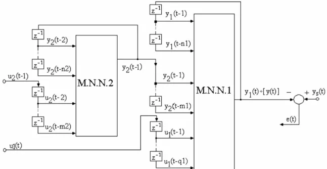
The block schema of the system represented in figure no.1 suggests the following neural structure (figure no.3) for the system’s identification.

Because the suggested structure contains internal elements of delay and memorising, the neural network will be called internal recurrent neural network. The two neural networks will identify the subsystems 1 (M.N.N.1) and the subsystem (M.N.N.2).

Using a neural network with a structure identical to the system, the neural network is able to capture the dynamics of the given system.

Another advantage of this neural structure (figure no.3) is that it allows the determination of the neural models of the component sub-systems. The suggested neural structure can estimate the internal variables of the system without measuring them.

If it is known the neural model of a sub-system, then this can be used in the learning stage of the other neural sub-systems.

In the following paragraph there are presented the aspects regarding the identification of the systems using internal recurrent neural networks.

(3)

3.INTERNAL RECURRENT NEURAL NETWORKS

In this section there are presented the aspects regarding the learning of a neural network which identifies a system with a single input and a single output. To simplify, it is considered that the system contains two subsystems.

In figure no. 5 it is shown the schema of an internal recurrent neural network which contains two recurrent neural networks.

Each neural network approximates a nonlinear function given by an expression such as:

)

x

,...,

x

,

x

(

f

y

_n

=

_n ₁ ₂ _r , where:

• ;

))

1 q

t

(

u

),...,

1 t

(

u

)

1 m

t

(

y

),...,

1 t

(

y

)

1 n

t

(

y

),...,

1 t

(

y

(

)

x

,...,

x

,

x

(

1 1 2 2 1 1 1 q 1 m 1 n 2 1

−

=

+ +

)

t

(

y

)

t

(

y

_n

=

₁ for neural network MNN1,

•

)

2 m

t

(

u

),...,

2 t

(

u

)

2 n

t

(

y

),...,

2 t

(

y

(

)

x

,...,

x

,

x

(

1 1 2 2 2 m 2 n 2 1

−

=

+ ;

for neural network

M.N.N.2.

)

1 t

(

y

)

t

(

y

_n

=

₂

−

The equations used to learn the M.N.N.1 and M.N.N.2 neural networks are the same with equations used to learn the back propagation neural networks (E. D. Rumelhart et. al., 1995).

To exemplify the relations which adjusts the parameters of the two networks it is considered the neuron output m which belongs to layer q of neural network k (k=1 for neural network 1 or k=2 for neural network 2). This output is calculated by the following formula: 1 1 ( ) ( ( , ) ( ), ( )) q Sk

q q q q q

n

Ak m Fk wk m n Ak − n Bk m

=

∑

⋅ (2)

where:

1

( )

q

Ak − n represents the neuron output n which belongs to layer (q-1) from network k ;

( , )

q

wk m n represents the connection between neuron m from layer q and neuron n from layer (q-1) of network k;

( )

q

Bk m represents the bias of neuron m from layer q of network k;

represents the activation function of neurons from layer q of network k;

(.,.)

q

Fk

represents the number of neurons from layer q of network k.

q

Sk

For the parameters adjustment it is used the method of decreasing gradient which minimises the following error criterion:

(3) 2

( ( ) ( )) Er= y t −ys t

With these notations and considering the relation (2) are obtained the following equations which adjusts the parameters of the network:

1 1

1 ( , ) 1 ( , ) 1( ) 2 1 ( ) 1

1 ( ) 1 ( ) 1( ) 2 1 ( )

q

qkp qkp q

i q

qkp qkp

w i j w i j kp e j A

B i B i kp e j

η η + − + − ⎧ = − ⋅ ⋅ ⎪ ⎨ = − ⋅ ⋅ ⎪⎩ ⋅ (4) where 1 ₁ 1 1

1 ( ) 1 '( 1 ( ), 1 ( )) ( ( ) ( )) 1 ( ) 1 '( 1 ( ), 1 ( )) ( ) 1 ( , ) 1

n n n n

S q

q q q q q q

p

e j F X j B j y j ys j

e j F X j B j e p w j p

q n + + = ⎧ = ⋅ − ⎪⎪ ⎨ = ⋅ ⋅ ⎪ ⎪⎩ ≤ <

∑

(5) 1 1 1 1

1 ( ) 1 ( , ) 1 ( )

q S

q q q

n

X m w m n A n

−

− =

=

∑

⋅ , m=1, 1S q

⋅

η1(kp) learning rate for neural network 1.

1 1

2 ( , ) 2 ( , ) 2( ) 2 2 ( ) 2 2 ( ) 2 ( ) 2( ) 2 2 ( )

q

qkp qkp q

i q

qkp qkp

w i j w i j kp e j A

B i B i kp e j

η η + − + − ⎧ ₌ ₋ _{⋅ ⋅} ⎪ ⎨ = − ⋅ ⋅ ⎪⎩ (6) where 1 1 1 1 1 2 ₁ 1 1

2 ( ) 2 '( 2( 1), 2 ( )) 1 ( ) 1 ( , )

2 ( ) 2 '( 2 ( ), 2 ( )) 2 ( ) 2 ( , )

1

S

n n n

p S q

q q q q q q

p

e j F y t B j e p w p i

e j F X j B j e p w j p

q n = + + = ⎧ ⎪ = − ⋅ ⋅ ⎪⎪ ⎨ ⎪ = ⋅ ⋅ ⎪ ⎪⎩ ≤ <

∑

(7) 1 1 1 1

2 ( ) 2 ( , ) 2 ( )

q S

q q q

n

X m w m n A n

−

=

∑

⋅ , m=1, 2S q

η2(kp) learning rate for neural network 2. Observations

The M.N.N.2 neural network can have as many inputs and outputs and command variables as are specific to the analysed sub-system. In this situation, the dimension of the input vector increases, while the scientific approach remains unchanged.

(4)

sub-system that is approximated to the neural network 2 (M.N.N.2) is not known, then the learning of the two networks must be done simultaneously.

In order to present the way of processing the data and the way of the propagation of the error through the internal recurrent neural structure (figure no.4 and figure no.5), the following hypotheses are presumed:

• the M.N.N.1 and M.N.N.2 neural networks have a single neuron of the output layer with the

linear activation function;

• the connection between the two networks is in fact the connection between the output of the M.N.N.2 network and the input on the position i - {x(i)} of the M.N.N.1 network;

• the input layer of the M.N.N.1 network has q neurons.

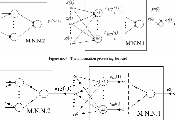
The way of the information processing forward through the network and the way of the backward error propagation is illustrated in the following figures.

Figure no.4 - The information processing forward

Figure no.5 - The backward error propagation In the figures above there are represented only the

variables that are needed in the internal recurrent neural networks presentation. The significations of the variables are:

• y2(t-1) output of the M.N.N.2 that becomes the input {x(i)} of the MNN1 neural network;

•

( x( 1 ), x( 2 ),..., x( r ))

the inputs of the M.N.N.1 neural network ;

• the neurons

outputs of the last layer of the M.N.N.1 neural network;

us us us

( A ( 1 ), A ( 2 ),..., A ( q ))

• y(t) ,ys(t) and e(t) represent the network output, the system output and the error;

• e12(i,t) represents the error e(t), that it is propagated through the M.N.N.1 neural network;

• represents the error e(t), that is the backward propagation through neuron j from the last layer of the M.N.N.1 neural network.

us j=1,q

{e (j)}

The error which is propagating through these neural networks (M.N.N.1 and M.N.N.2) is:

• e( t )=( y( t )−ys( t )) for M.N.N.1 neural network;

•

nern2 nern2

us us p 1

e12( i,t ) F '( y2( t 1 ),B ) q

e ( p ) w ( p,i )

=

= − ⋅

⋅

∑

for MNN1

neural network.

(5)

following significations:

• nern2

F - represents the activation function of the output neuron of the M.N.N.2 network ;

•

B

nern2 - the bias of the output layer neuron of the MNN2 network;

• - represents the weight between input i [ x(i)] and p neuron of the M.N.N.1 network last layer.

us

w ( p,i )

The neural structure from figure no. 3 has two major advantages:

• the possibility to configure the neural network depending on the system structure. Also the neural structure used allows the application of the input variables to the hidden layer;

• the possibility of the neural structure learning without knowing the output variable of the sub-systems. This advantage allows to design an estimator of the sub-system output;

The neural structure suggested in figure no. 3 needs a specific algorithm, because the input of the

M.N.N.2 network (

modifies itself with each learning stage. In this situation, after each adjustment of the M.N.N.2 network weigths, the input vector of the neural M.N.N.2 will be modified.

y2( t−2 ),..., y2( t−n2 ))

4.IDENTIFICATION OF THE SYSTEM USING INTERNAL RECURRENT NEURAL

NETWORKS

In this paragraph there are presented the practical

aspects regarding the identification of the system with internal recurrent neural networks.

For the case study there are used the following equations which describe the systems represented in figure no.1 1) (k y 1 1) (k y 1 1)) (k u 1) (k (y 1) (k y 1) (k y 1.2 1 1) (k y 4 (k) y 2 1 1 1 1 2 2 1 1 1 − + − + ⋅ − + − + + − + − ⋅ + − ⋅ = (8) ] ) k ( y ( ) k ( u ) k ( u ) k ( y [ . ) k ( y 1 1 1 2 1 1 5 0 2 2 2 2 2 2 − + ⋅ − ⋅ + + − + − − ⋅ =

.

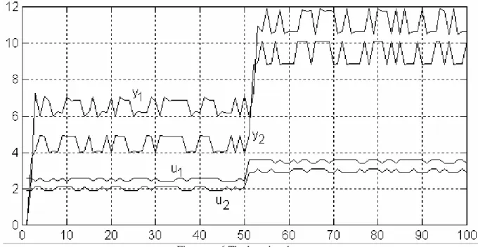
The learning data are presented in figure no. 6 and the data set which is used to learn the internal recurrent neural network is given below.

} )) i ( y ) i ( u {( P t nl , i 3 1 1 1 1 0

1= − − ₌

} )) i ( u {(

P2= 0 2 −2 _it₌₃_,_nl } )) i ( y {( T nl , i 3 1 ₌ =

Initially, the first line of the P2 matrix is zero, and the values of the first line will be modified after each learning step. Also, the values of the first line of the P1 matrix are zero initially, but after the learning stage these are set to the values of the M.N.N.2 output.

(6)

The structures of these two neural networks are: The M.N.N.2 neural network has three layers:

• layer 1- 3 neurons and activation function tan-sigmoid,

• layer 3- 1 neuron and activation function linear.

The M.N.N.1 neural network has three layers, too:

• layer 3- 1 neuron and activation function linear.

The parameters of the neural networks are initialized with random sequence.

In the following, there are presented the computed steps of the neural network learning stage.

The learning algorithm

1. It is initialized the j counter with 1;

2. It is computed the M.N.N.2 ( y2(j)) output network with the following:

t RN 2

y2( j )= f [( P2( 1, j ) P2( 2, j ) P2( 3, j )) ] where fRN 2 represents the non-linear function

identified by M.N.N.2 neural network;

3. It is brought up to date the learning lot by the next step :

2 2

P2( 1, j

+

1 )

=

y ( j ),

P1( 2, j )

=

y ( j );

4. It is computed the output MNN1 network:

y( j )

=

f

RN 1

[( P1( k , j )

k 1,10=

) ]

t

where fRN 1 represents the non-linear function

identified by M.N.N.1 neural network; 5. It is computed the error e(j)=T(j)-y(j);

6. It is adjusted the M.N.N.1 network parameters by backwards propagation of the error e(j);

7. It is computed the error e12(2,j) propagated through MNN1 neural network and through the connection from the MNN2 network output and the M.N.N.1 network input-2.

8. It is adjusted the M.N.N.2 network parameters by backwards propagation of the error e12(2,j);

9. It is increased the j counter j=j+1;

10. If j<nl (nl-the size of the learning data), then jump to step 2, otherwise continue;

11. STOP.

This algorithm is different from the classic algorithm because it contains the 3 and 7 steps. Through these steps, the learning data are continuously modified.

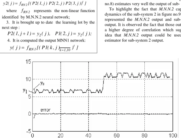
After the learning stage, the output of the M.N.N.1 neural network and the output system are illustrated in the figure no.7.

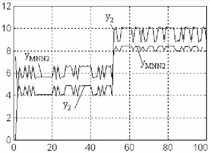
In order to verify the capacity of generalisation, it is used a data set different from the learning data. It can be noticed the fact that the network output (figure no.8) estimates very well the output of sub- system 1. To highlight the fact that M.N.N.2 captures the dynamics of the sub-system 2 in figure no.9, there are represented the M.N.N.2 output and sub-system 2 output. It is observed the fact that those outputs have a higher degree of correlation which suggests the idea that M.N.N.2 output could be used like an estimator for sub-system 2 output.

(7)

Figure no.8 The M.N.N.1 output and sub-system 1 output

Figure no.9 The M.N.N.2 output and sub-system 2 output

5.CONCLUSION

Internal recurrent neural network structures suggested in this paper represent a contribution to the identification system fields with neural networks.

This approach has the following features:

• using a neural network with a structure identical to the system’s structure, the neural network is able to capture the dynamics of the given system.

• the possibility of independently learning, every neural network if the data learning is available;

• the neural network structure can estimate the internal variables of the analysed system;

• if it is known the neural model of a sub-system, then this can be used in the learning stage of the other neural sub-systems.

6. REFERENCES

S. P. Satry, et. al. (1994) , “ Memory Neuron Networks for Identification and Control of Dynamical Systems ” , IEEE Neural Networks Vol. 5 No. 2.

D. Pham and L. Xiug, (1995), “Dynamic System Identification Using Elman and Jordan Networks, Neural Networks for Chemical Engineers”, Editor A. Bulsori, Chap. 23.

(8)

E. D. Rumelhart, E. G. Hinton, and J. R. Williams, (1995) “ Learning Internal Representation by Error Propagation ” , in Parallel Distributed Processing. Vol. 1, MIT Press, Cambridge. Chung-Ming Kuan, (1995 ), “A Recurrent Newton

Algorithm and Its Convergence Properties” IEEE on Neural Networks Vol. 6 No. 3.

J.Liang and M. M. Gupta (1999), “Stable Dynamic Backpropagation Learning in Recurrent Neural Networks” IEEE on Neural Networks Vol. 10 No. 6.