F. D. Marques
L. de F. Rodrigues de Souza
D. C. Rebolho
A. S. Caporali
and E. M. Belo
Aeroelasticity, Flight Dynamics and Control Lab Engineering School of São Carlos – USP Av. Trabalhador Sancarlense, 400 13566-590 São Carlos, SP. Brazil [email protected] [email protected] [email protected] [email protected] [email protected]R. L. Ortolan
Biocybernetics & Rehabilitation EngineeringSchool of São Carlos – USP Av. Trabalhador Sancarlense, 400 13566-590 São Carlos, SP. Brazil [email protected]
Application of Time-Delay Neural and
Recurrent Neural Networks for the
Identification of a Hingeless
Helicopter Blade Flapping and
Torsion Motions
System identification consists of the development of techniques for model estimation from experimental data, demanding no previous knowledge of the process. Aeroelastic models are directly influence of the benefits of identification techniques, basically because of the difficulties related to the modelling of the coupled aero- and structural dynamics. In this work a comparative study of the bilinear dynamic identification of a helicopter blade aeroelastic response is carried out using artificial neural networks is presented. Two neural networks architectures are considered in this study. Both are variations of static networks prepared to accomodate the system dynamics. A time delay neural networks (TDNN) for response prediction and a typical recurrent neural networks (RNN) are used for the identification. The neural networks have been trained by Levemberg-Marquardt algorithm. To compare the performance of the neural networks models, generalization tests are produced where the aeroelastic responses of the blade in flapping and torsion motions at its tip due to noisy pitching angle are presented. An analysis in frequency of the signals from simulated and the emulated models are presented. In order to perform a qualitative analysis, return maps with the simulation results generated by the neural networks are presented.
Keywords: System identification, helicopter blade, time delay neural networks, recurrent neural networks.
Introduction
Aeroelastic instabilities are factors that can limit aircraft capacity of flight and, therefore, must be carefully examined during the design and development stages of any aircraft. Modern fixed- and rotary-wing aircraft are requested to fly at higher speeds and to have less weight, thus increasing its structural flexibility. Therefore, a safe analysis of the fluid-structure interactions must be taken in order to obtain a dynamic model presenting all these relevant characteristics (Belo and Souza, 2001).1
The helicopters are aircraft with rotating wings, which leads to complex aeroelastic features. An example is the helicopter main rotor blades that are thin and flexible and then, even in normal operation conditions can undergo large elastic deformations. Such effects can lead to treatment beyond the theoretical limits considered by linear beams hypothesis (Celi, 1999). These and other factors make the linear models inadequate for the necessary analyses for rotorcraft aeroelasticity. Consequently, linear models are substituted by non-linear ones. This procedure has been facilitated by the increasing availability of faster and more powerful computers. However, the mathematical modelling of non-linear systems is considerably more complex than linear ones, becoming some times impracticable for short-term and even some times, unfeasible.
Due to the difficulty in representing non-linear systems by analytical models, there has been an increase of works on identification system. System identifcation is the process of finding a model of a physical system given input-output measurements. It is commonly referred to as an inverse problem, because it is the opposite of the problem of computing the response of a system with known characteristics. Non-linear system identification is a much younger discipline than linear system identifcation and the theory for the nonlinear case is often an extension of the linear case.
Paper accepted May, 2005. Technical Editor: José Roberto de F. Arruda.
Some novel representations used in the modelling of non-linear systems are: i) neural networks; ii) functions of radial base; iii) Volterra Series; iv) Wavelets transforms; v) polynomial and rational functions and vi) polynomial differential equations. It is worth noticing that bilinear models constitute a special class of non-linear polynomial models (Aguirre et al., 1998).
According to Cruz (1998), Artificial Neural Networks have been considered a powerful identification tool, allowing the modelling of the processes from their input and output data. Beyond all advantages, neural networks possess reasonably high processing speed as compared to other conventional methods, as well as learning capacity in some way similar to the human one.
Narendra and Parthasarathy (1990) have presented a comprehensive study on the applicability of multilayer neural networks for identification and subsequent use to control non-linear dynamic systems. Takahashi (1999) has presented a multilayer neural network trained by using the backpropagation algorithm to detect the critical aerodynamic loading for the occurrence of flutter and the limit conditions in the structure. Maghami et al. (2000) have
presented a new procedure for developing and training artificial neural networks, useful for fast and efficient control as well as for the analysis of flexible space systems. In Greenwood (1997), the long time performance of the multilayer networks applied to the estimation of dynamic systems behaviour has been studied.
Giannakis et al. (2001) have presented a survey related to the
identification of non-linear systems and its applications. In Tsoi (1998), a quite complete review on recurrent neural networks can be found.
The blade has been modelled by the finite element method and a bilinear state space representation is produced. The mildly non-linear features of the binon-linear model are explored to achieve a database for further neural network training. Comparisons between the TDNN and RNN models are presented. A qualitative analysis of the models are proceeded by means of the respective construction of the return maps.
Helicopter Blade Non-linear Mathematical Model
The hingeless helicopter blade is modelled as a rotating cantilever beam with length R, undergoing the coupling motions of
flapping, lead-lagging, axial stretching and torsion. Detailed modelling aspects have been presented in Marques (1993). Figure 1(a) shows the main coordinate system x, y and z, that is fixed to the blade root with its origin in the intersection of the blade root cross-section and the elastic axis. When the blade is not deformed the x
-axis is exactly coincident with the elastic -axis. It is also supposed that elastic and mass axes are noncoincidents. Figure 1(a) also shows the deformed blade and elastic displacements u, v and w, in
the x, y and z directions, respectively. Figure 1(b) shows an arbitrary
blade cross-section and its local coordinate system η and ζ. A
pretwist angle θt and the torsional deflection φ can also be seen.
Elastic axis Elastic axis
(a)
Elastic axis Elastic axis
(b)
Figure 1. (a) Blade coordinate system and elastic displacement and (b) cross-sectional coordinate system (Marques, 1993).
Strain and Kinetic Energy
The strain energy, considering a rotating beam undergoing axial stress, shear in the lead-lagging plane and in the flapping plane, is given by (Marques, 1993):
(
)
{
(
)
}
dx w F v F GJw v EI w
v EI u EA U
c c
t t
y R
t t
z
2 2 2
2
0
2 2
cos sin
sin cos 2
1
′ + ′ + ′ +
′′ + ′′ − + ∫ ′ + ′′ + ′′ =
φ
θ θ
θ θ
(1)
where, EA, EIy, EIz and GJ are the axial, lead-lagging, flapping and torsional stiffness, respectively. The term Fc is the centrifugal effect and is a function of the mass (m) and the blade rotational
speed (Ω), that is:
∫Ω =R
x
c mxdx
F 2 (2)
The kinetic energy equation is given by:
(
)
dxdt r d dt
r d d d T
R
A
∫
⎭ ⎬ ⎫ ⎩
⎨ ⎧
∫∫ ⎟
⎠ ⎞ ⎜ ⎝ ⎛ ⋅ =
0
2
1 ρ η ζ G G
, (3)
where,
dt
r
d
G
is the velocity vector of an arbitrary point in the bladecross-section.
Aerodynamic Loading
A quasi-steady aerodynamic approach has been adopted to yield the expressions of lift (L), drag (D) and aerodynamic moment (M) in the hovering flight condition (Marques, 1993). The induced velocity, which yields a free airflow velocity parallel to the y-axis,
has been neglected. The small displacement consideration results in the assumption that the blade cross-section remains parallel to the yz
plane. Mass and elastic axes are not coincident, but the aerodynamic centre is taken at the same point of the elastic axis and cross-section intersection. The NACA 0015 airfoil has been assumed, which leads to coincident blade cross-section aerodynamic and pressure centres.
A blade element dx has been taken and the corresponding load
element has been computed. Considering that the blade elastic displacements in the free air flow and an operational region for the blade angle of attack, the aerodynamic loading results:
(
)
{
[
]
(
)
[
v x u]
w}
dxv u e
C C C c M
L D
R
x
t P
L L D
ar
2 2
2 0
2 1
+ + Ω + +
+ Ω − ∫ +Θ + + ⎥
⎥ ⎥
⎦ ⎤
⎢ ⎢ ⎢
⎣ ⎡ =
⎥ ⎥ ⎥
⎦ ⎤
⎢ ⎢ ⎢
⎣ ⎡
φ θ θ
ρ
α α α
(4)
where, e is the offset between elastic and mass axis; ρarar is the air mass density; c is the blade cross-section chord; θp is the command
pitch angle; Θ
0 is the nominal value of pitch angle in the operational region (10° maximum).
Proper linearization can be achieved by supposing, for instance, small displacements and neglecting higher order terms. Nonetheless, it is desired to maintain some degree of non-linearity. Here, mildly non-linear effect can be attained by keeping coupling terms, such as those relating the states and input variables.
Finite Element Model and Bilinear Representation
The finite element discretization is proceeded in terms of beam elements with six degrees of freedom per node, viz: displacements in
the x, y and z directions, rotations in the xy, xz planes and in the cross-section plane. The nodal displacements (generalized
coordinates) form the q vector and are related with blade
2 2 1 1 2 6 2 5 1 4 1 3 2 6 2 5 1 4 1 3 2 2 1 1 φ φ
φ H (x) H (x)
w ) x ( H w ) x ( H w ) x ( H w ) x ( H w v ) x ( H v ) x ( H v ) x ( H v ) x ( H v u ) x ( H u ) x ( H u + = ′ + + ′ + = ′ + + ′ + = + = (5)
where, H1(x) through H6 (x) are the shape functions given by the
Hermitian polynomials and the subscripts 1 and 2 are related to the displacements at each element node.
The mass, gyroscopic, and stiffness matrices, Me, Ge and Ke, of
each finite element have their respective coefficients mij, gij and kij, for i,j = 1,2,...n, that are obtained by substituting Eq. (5) into Eqs.
(1) and (3). However, these coefficients are not linear in q.
Linearization occurs by using small motion assumption about the equilibrium point, which yields the following expressions (Marques, 1993): 0 q 2 0 q 2 0 q 2 0 q 2 0 q 2 q q q q , q q q q , q q = = = = = − = − = = j i j i ij j i i j ij j i ij T U k T T g T m ∂ ∂ ∂ ∂ ∂ ∂ ∂ ∂ ∂ ∂ ∂ ∂ ∂ ∂ ∂ (6)
Superposing each Me, Ge and Ke, respectively, and considering
the system constraints, the global system matrices are assessed. Damping effects have been introduced to the model by using the Rayleigh approach and a damping factor ξ = 0.05 (Marques, 1993).
By substituting Eq. (5) into Eq. (4), non-linear loading equations are obtained and simplified. The coupling between the generalized coordinate vector q and the input variable θ (blade pitching angle) has been kept in the model in order to provide some degree of non-linearity. The final blade mathematical model results in the following equation of motion in matrix form:
(
G C)
q Kq Q(q,q,qθ,θ) qM+ + a + = (7)
where, q is the nodal displacement vector, M, G, Ca, K are the
global mass, gyroscopic, damping, and stiffness matrices, respectively, Q is the aerodynamic loading matrix and θ is the blade pitching angle.
The presence of coupled terms (system states and input variable) allows bilinear system representation. Bilinear systems (Mohler, 1991) are systems that present linear behaviour in state and linear behaviour in control, but they are not jointly linear in state and control, because products of state and control are involved. They comprise one of the simplest class of non-linear systems, and they can be produced from slight generalisations of linear systems. Nonetheless, with such systems the superposition principle is not applicable. The equation of motion given by Eq. (7) can, then, be conveniently transformed into state-space representation, resulting:
[
Qx Qu Q xu]
B x A
x= + 1 + 2 + 3 (8)
where, x is the state vector, u is the input or control vector, A is the state matrix, B is the control matrix, Q1 is the aerodynamic loading
matrix with the coefficients depending on the systems states, Q2 is
the aerodynamic loading matrix with the coefficients depending on
the inputs and Q3 is the aerodynamic loading matrix with the
coefficients depending on the coupling between system states and inputs. By grouping the terms, the traditional state-space representation form is obtained, that is:
xu N u B x A
x = 1 + 1 + , (9)
where, A1=A+BQ1, B1 =BQ2 , N=BQ3, with N being the
bilinear coupling matrix (u = θ).
Artificial Neural Networks
Artificial neural networks are information processing systems with the capability of learning through examples (Haykin, 1994). Based on concepts derived from neuro-biology, neural networks are composed by a set of interconnected processing units, called
neurons. The neurons process the signals presented to the neural network by accumulating each stimulus and by transforming the total value using a function; that is, the activation function. The stimuli to and from a neuron are modified by the real value called
synaptic weight, which characterises the respective connection between neurons.
Figure 2 shows a typical representation for a generic neuron j, where x1, x2, ..., xp are the stimulus signals, wj1,wj2,...,wjp, are the synaptic weights, θj is a bias value, vj is the activation potential, oj is
the neuron output signal, and ϕ(.) is the activation function
(generally adopted as a non-linear sigmoid function).
Figure 2. Typical neuron representation.
Then, from Figure 2, one can observe that the neuron output is given by: ⎟⎟ ⎟ ⎠ ⎞ ⎜⎜ ⎜ ⎝ ⎛ + =
∑
= p i i ji jj w x
o
1
θ
ϕ (10)
Network architecture is the name given to the arrangements of
neurons into layers and how they are connected. Typical neural networks have the following architecture: (1) input layer – where
the input stimulus is presented to the network; (2) hidden layers –
internal layers of a network, and (3) output layer – the last layer of
the network, where the outputs are given. Such typical network
architecture is commonly referred to as a multi-layer neural
network.
Once trained, one can assume that the network stored the knowledge supplied to it. However, the knowledge in a neural network is not stored in a particular localization. It depends on its topology and the magnitude of the weights in the input layer.
The generalization of an artificial neural network is the capacity to reproduce desired signals for different input signals that have not been used during the network training, or either, that it is able to catch the dynamics of the system being emulated (Saravanan & Duyear, 1994).
Recurrent Neural Networks (RNN)
other words, models based on past values of the system input and output.
Recurrent networks (RNN) are neural networks with one or more feedback connections that can be of local or global nature. Feedback allows the recurrent networks to acquire state representations, making them appropriate devices for different dynamic applications such as: forecasting or modeling non-linear systems, adaptive equalization of communication channels, control of industrial installations, diagnostic of automotive engines and processing of temporal signals as the voice signal (Haykin, 1994).
In RNN’s both feedforward and feedback (recurrent) connections between neurons are allowed (Kling, 2003). As with ordinary multilayer perceptrons, recurrent multilayer perceptrons can perform any nonlinear mapping, but the difference is that the response to an input from a recurrent network is now based on all previous inputs, as these are used in feedback connections. Nonetheless, the recurrent network is a dynamic system, with the activations of the neurons with feedback connections being the state of the system.
The output of a RNN network is a function of the current external input together with its previous inputs and outputs as given by:
y(k)=f(u(k),u(k−1),...,u(k−M),y(k−1),y(k−2),...,y(k−N)) (11)
Time Delay Neural Networks (TDNN) are a particular case of recurrent neural networks. The response of these neural networks in time t is based on the inputs in times (t-1),(t-2), ..., (t-n). A mapping
performed by the TDNN produces a y(k) output at time k as:
)) M k ( u ),..., k ( u ), k ( u ( f ) k (
y = −1 − (12)
where u(k) is the input at time k and M is the maximum adopted
time-delay.
After been adequately trained, TDNN have been used successfully for prediction, because they are able to capture the
dynamics of a
system and to foresee the output in the current
time.
Neural Network Training
To achieve a desirable set of synaptic weights to a pre-defined network architecture, a training process is needed. A training process is generally based on an optimisation scheme to adjust the network parameters (mainly, the weights) in relation to a set of input-to-output to be matched by the neural network model (supervised learning scheme). The backpropagation algorithm based on a gradient descent technique (Haykin, 1994) has been widely applied for general neural network training. More efficient training scheme can be achieved by using the Levenberg-Marquardt Algorithm (LMA).
Levenberg-Marquardt Algorithm (LMA)
This algorithm is a variation of the Newton’s method for minimizing functions that are sums of squares of other non-linear
functions (Hagan et al., 1996). The LMA provides better
performance when compared with typical backpropagation algorithms.
From Newton’s method the network update rule is:
n n n
n w H g
w +1= − −1 , (13)
where, w is the network weight matrix, n is a step of iteration, H is the Hessian matrix and g is the gradient matrix.
For the performance index as a sum of squares functions, the Hessian matrix can be approximated in terms of the Jacobian matrix, J, which contains first derivatives of the network errors with respect to the weights and biases. Thus,
J J
H≅ T . (14)
When the approximation in Eq. (14) is substituted into Eq. (13), the Gauss-Newton method is obtained, that is:
[ ]
n n nn
n w J J g
w +1= − T −1 . (15)
A problem that may arise in the Gauss-Newton method is that the matrix [JTJ] may not have an inverse. This can be overcome by assuming a modification to the matrix [JTJ] that leads to the LMA:
[
n n n]
nn
n w J J I g
w +1= − T +µ −1 , (16)
where, I is the identity matrix and µ is a scalar.
The scalar µ presents an important role to the LMA. When µn is zero, the weight update is basically the Gauss-Newton method. When µn is sufficiently large, Eq. (16) becomes gradient descent
with small step size. By choosing the proper value of µ the LMA
provides an efficient compromise between the great performance of the Newton’s method and the guaranteed convergence of the gradient descent approach.
Identification of Helicopter Blade Non-Linear Dynamics
This work presents an approach for non-linear dynamics identification and prediction of a rotating helicopter mathematical
model blade. It has been considered a blade with length of 4.09m
and mass distribution of 2.3kg/m (Marques, 1993). The flight
condition is hovering with the rotor spinning at 360 rpm. Other
problem parameters are: axial stiffness - EA=5.09×10⁷N; shifting
between CG and elastic axis - e = -0.01013m; torsional stiffness -
GJ = 2.28×10⁴Nm; flapping stiffness - EIy = 3.22×10³ Nm2;
lead-lagging stiffness - EIz = 1.18×10⁵Nm2; radius of gyration -
km1=0.008Ns2; km2=0.04Ns2.
The blade has been also considered as a cantilever rotating beam subjected to flapping, lead-lagging and torsion displacement. The mathematical model has been represented in the bilinear form, as given by Eq. (9). The helicopter blade bilinear model has been obtained from finite element discretization using 5 elements. It has been considered the lowest level of discretization, in which the model presents proper system response representation.
To obtain sets of input-output pairs, that is, necessary data for the training of the networks, the blade bilinear model has been simulated using random inputs (frequency varying from 0 to 10 Hz).
Some simulations have been made considering the blade operating with a pitch angle of 5 degrees.
Two artificial neural networks topologies have been trained. First, a feedforward multilayer neural network with delays in time (TDNN) has been trained. The predictive model follows the model described by Eq. (12). To train the neural network, the current and previous signals of the blade rotation, as well as the previous flapping and torsion signals at the blade tip, have been used to
estimate flapping and torsion in the current instant. The TDNN
topology presentes has three layers: an input layer (16 neurons), an
output layer (2 neurons) and an hidden layer (10 neurons). Linear
A recurrent network (RNN) as described by Eq. (11) has been also implemented. The RNN network topology has been taken with three neuron layers, linear and tangent sigmoidal activation functions and 13, 2 e 6 neurons, respectively, in the input, output and hidden layers.
After training, the TDNN error decay has reached a value as low as 10-5 and it was stabilized after 20 epochs. Similarly, the RNN
training error decay has reached the order of 10-6 and stabilized after
10 epochs, as can be observed in Figure 3.
Training results have revealed a good matching between training samples and network outcomes. Those results have been omitted from this paper for the sake of conciseness. It has been considered more relevant to present the generalization features of the neural networks. A more complete analysis of the training has been presented in Souza (2002).
Figure 4 show the results of generalization tests that were carried out with TDNN and RNN network models.
In these tests, it can be observed that has been used a random-type input and the results reveal that the generalization has been sufficiently satisfactory. The results also revealed that both the neural network models have better identified the torsion motion. As far as the flapping motion is concerned, discrepancies have been more evident for either TDNN and RNN models.
0 5 10 15 20 25 30 35 40 45 50
10-5 10-4 10-3 10-2 10-1 100 101
Epochs
E
rror d
e
c
a
y
TDNN RNN
Figure 3. Error decay comparison after training the TDNN and RNN.
0.5 0.55 0.6 0.65 0.7 0.75 0.8 0.85 0.9 0.95 1 -4
-2 0 2 4x 10
-3
F
lapp
in
g [
m
]
Simulated TDNN RNN
0.5 0.55 0.6 0.65 0.7 0.75 0.8 0.85 0.9 0.95 1 -1
-0.5 0 0.5 1
T
o
rs
io
n
[
deg
re
e]
Simulated TDNN RNN
0.5 0.55 0.6 0.65 0.7 0.75 0.8 0.85 0.9 0.95 1 -1
-0.5 0 0.5 1
P
it
c
h [
d
egree
]
Time [s]
Figure 4. Flapping and torsion motions at the blade tip for the RNN and TDNN networks simulation.
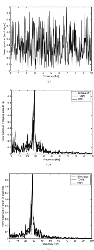
Using the identification results obtained from these tests, the signals have been analyzed in the frequency domain. Figure 5(a) to 5(c) show the frequency spectrum of the input signal (Fig. 5(a)), flapping response (Fig. 5(b)), and torsional response (Fig. 5(c)). The normalized power spectra from simulated and emulated response by the TDNN and RNN models ensure that the network models are capable of capturing the system frequency contents.
0 1 2 3 4 5 6 7 8 9 10
0 0.1 0.2 0.3 0.4 0.5 0.6 0.7 0.8 0.9 1
Frequency [Hz]
P
o
w
er
s
pec
tr
um
(
inpu
t s
ig
nal
)
(a)
0 10 20 30 40 50 60 70 80 90 100 0
0.1 0.2 0.3 0.4 0.5 0.6 0.7 0.8 0.9 1
Frequency [Hz]
P
o
w
er
s
p
ec
tr
um
(
F
lapp
ing
i
n bl
ad
e t
ip)
Simulated TDNN RNN
(b)
0 10 20 30 40 50 60 70 80 90 100 0
0.1 0.2 0.3 0.4 0.5 0.6 0.7 0.8 0.9 1
Frequency [Hz}
P
o
w
e
r s
pec
tr
um
(T
or
s
io
n
i
n
bl
ade
t
ip
)
Simulated TDNN RNN
(c)
Figure 5. (a) Frequency spectrum of input signal. (b) Frequency spectrum of blade tip flapping response. (c) Frequency spectrum of blade tip torsion response.
response. Figure 5(c) also shows frequency spectra as in Fig. 5(b), but now considering the blade tip torsional response. One can verify that the frequency content in the simulated response is identified in the TDNN and the RNN responses.
A qualitative analysis of the neural networks responses time histories are also proceeded in terms of methods for threating time series. Accordingly to Greenwood (1997), a dimension map is given by a function that is represented by:
] M[ (n)
1) (n
x
x + = (17)
where, x(n) is the value of x for time n and a particularly simple
example, and for this reason one of the most used two-dimensional maps, is the Return Map. Given x(n) of any time series, the Return Map is the evolutuion x(n) against x(n+1) as a function of time. Such plotting shows how complex may be the System behaviour
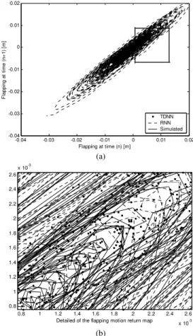
Figure 6(a) presents a comparison between the return maps of flapping motions at the helicopter blade tip generated by simulation with, respectively, the results generated by the neural network with delays in the time (TDNN) and the recurrent one (RNN) and Fig. 6(b) shows a detailed area of Fig. 6(a), where one can see how the return maps are contained in the same orbit region. Analogly, Figs. 7(a) and 7(b) present the same comparison, but now for the torsion response.
One can observe that, either the maps plotted with the simulation results or the maps plotted with the results generated by the networks, are quite similar, which means that identification quality is good, i.e., both TDNN and RNN neural networks have provided satisfactory identification models.
-0.04 -0.03 -0.02 -0.01 0 0.01 0.02 -0.04
-0.03 -0.02 -0.01 0 0.01 0.02
Flapping at time (n) [m]
F
lap
pi
ng
a
t t
im
e
(n
+
1
) [
m
]
TDNN RNN Simulated
(a)
0.8 1 1.2 1.4 1.6 1.8 2 2.2 2.4 2.6 x 10⁻³ 0.8
1 1.2 1.4 1.6 1.8 2 2.2 2.4 2.6
x 10-3
Detailed of the flapping motion return map (b)
Figure 6. (a) Flapping motion return map. (b) Detailed of the flapping motion return map.
-2.5 -2 -1.5 -1 -0.5 0 0.5 1 1.5 2 2.5 -2.5
-2 -1.5 -1 -0.5 0 0.5 1 1.5 2 2.5
Torsion at time (n) [d]
T
o
rs
io
n at
t
im
e
(
n
+
1
) [
d
]
TDNN RNN Simulated
(a)
-0.75 -0.7 -0.65 -0.6 -0.55 -0.5 -0.7
-0.65 -0.6 -0.55 -0.5 -0.45 -0.4
Detailed of the torsion motion return map (b)
Figure 7. (a) Torsion motion return map. (b) Detail of the torsion motion return map.
Conclusions
This work has presented an application of artificial neural networks in the identification of a hingeless helicopter blade flapping and torsion aeroelastic motions. The blade has been modelled by the finite element method and a bilinear state space representation has been produced. Two neural networks architecture has been considered: a time-delay neural network (TDNN) for response prediction and a recurrent neural network RNN for identification. Comparisons between the TDNN and RNN have been presented.
It has been observed that the RNN model needed a lesser number of neurons in hidden layer that the TDNN. It has allowed lesser time to train the RNN and it is has reached lower error level. However, after adequately trained, both neural networks have provided satisfactory results.
Generalization tests have been carried out and the results have been also satisfactory. An analysis in frequency domain with of both simulated and emulated models has been presented. One can be verify that the frequencies found in the simulated response are contained in the TDNN and the RNN responses, ensuring that the networks models are capable of capturing the system frequency contents.
TDNN and RNN neural networks have provided satisfatory identification models.
Acknowledgements
The authors wish to acknowledge the financial support of the Brazilian Research Agencies FAPESP, CNPq and CAPES, during the tenure of this research work.
References
Aguirre, L. A.; Rodrigues, G. G. and Jácome C. R. F., 1998, “Identificação de Sistemas não Lineares Utilizando Modelos NARMAX Polinomiais – Uma Revisão e Novos Resultados”, SBA Controle e Automação, Vol. 9, No. 2, pp 90-106 (in portuguese).
Belo, E. M. and Souza, L. F. R., 2001, “Identificação do Comportamento Não Linear de um Aerofólio Flexível”, In: 22nd Iberian
Latin-American Congress on Computational Methods in Engeering, Campinas, Brazil, (CD ROM – in portuguese).
Celi, R., 1999, “Recent Applications of Design Optimization of Rotorcraft”, A survey. 55th Annual Forum at the American Helicopter
Society, Montreal, Canada, May 25-27.
Cruz, J.C.G., 1998 “Identificação de Uma Torre de Retificação de Águas Ácidas Usando Redes Neurais Artificiais”. MSc Dissertation, Universidade Federal de Minas Gerais, Minas Gerais, Brazil (in portuguese).
Giannakis, G. B.; Serpedin, E., 2001, “A Bibliography on Nonlinear System Identification”, Elsevier Science, Vol.81, pp.533-580.
Greenwood, G. W., 1997, “Training Multiple-Layer Perceptrons to Recognize Attractors”, IEEE Transactions on evolutionary computational, Vol.1, No.4, p. 244-248.
Hagan, M.T.; Demuth, H.B.; Beale, M., “Neural Network Design”. PWS Publishing Co., 1996.
Haykin, S., 1994, “Neural Network: a Comprehensive Foundation”, Macmillan College Publishing Company, New York.
Kling, R. 2003. “An Implementation of Recurrent Neural Networks for Prediction and Control of Nonlinear Dynamic Systems”. MSc Thesis. Monash University in Melbourne in Australia.
Maghami, P. G. and Sparks, D. W., 2000, “Design of Neural Networks for Fast Convergence and Accuracy”, IEEE Transactions on Neural networks, Vol.11, n.1, pp.113-123.
Marques, F. D., 1993, “Controle de Vibrações em uma Pá de Helicóptero”. MSc Dissertation, Escola de Engenharia de São Carlos, Universidade de São Paulo, São Carlos, Brazil (in portuguese).
Mohler, R.R. (1991). “Nonlinear Systems”; Vol. 2, Applications to Bilinear Control, Prentice Hall, New Jersey, USA.
Narendra, K.P. and Partasarathy, K., 1990, “Identification and Control of Dynamical Systems using Neural Networks”, IEEE Transactions on Neural Networks, Vol. 1, pp. 4-27.
Saravanan, N.and Duyar, A., 1994, “Modeling Space Shuttle Main Engine Using Feed-Forward Neural Networks”. Journal of Guidance, Control and Dynamics, v. 17, n.4, pp.641-648.
Souza, L. F. R.2002. “Identificação da dinâmica não linear de uma pá de helicóptero via redes neurais”. MSc Dissertation, Universidade de São Paulo, Campus de São Carlos (in portuguese).
Takahashi, I. 1999, “Identification for Critical Flutter Load and Boundary Conditions of a Beam using Neural Networks”, Journal of Sound and Vibration, Vol.228, n.4, pp.857-870.