ISSN 1549-3644
© 2010 Science Publications
Corresponding Author: Noriszura Ismail, School of Mathematical Sciences, Faculty of Science and Technology, University Kebangsaan Malaysia, 43600 UKM Bangi, Selangor, Malaysia
Tel: +603 89215754 Fax: +603 89254519
Approximation of Aggregate Losses Using Simulation
Mohamed Amraja Mohamed, Ahmad Mahir Razali and Noriszura Ismail
Statistics Program, School of Mathematical Sciences, Faculty of Science and Technology,
University Kebangsaan Malaysia, 43600 UKM Bangi, Selangor, Malaysia
Abstract: Problem statement: The modeling of aggregate losses is one of the main objectives in actuarial theory and practice, especially in the process of making important business decisions regarding various aspects of insurance contracts. The aggregate losses over a fixed time period is often modeled by mixing the distributions of loss frequency and severity, whereby the distribution resulted from this approach is called a compound distribution. However, in many cases, realistic probability distributions for loss frequency and severity cannot be combined mathematically to derive the compound distribution of aggregate losses. Approach: This study aimed to approximate the aggregate loss distribution using simulation approach. In particular, the approximation of aggregate losses was based on a compound Poisson-Pareto distribution. The effects of deductible and policy limit on the individual loss as well as the aggregate losses were also investigated. Results: Based on the results, the approximation of compound Poisson-Pareto distribution via simulation approach agreed with the theoretical mean and variance of each of the loss frequency, loss severity and aggregate losses. Conclusion: This study approximated the compound distribution of aggregate losses using simulation approach. The investigation on retained losses and insurance claims allowed an insured or a company to select an insurance contract that fulfills its requirement. In particular, if a company wants to have an additional risk reduction, it can compare alternative policies by considering the worthiness of the additional expected total cost which can be estimated via simulation approach.
Key words: Aggregate losses, compound Poisson-Pareto, simulation
INTRODUCTION
Let X1, X2…, XN denote the amount of loss of an insurance portfolio that recorded N losses over a fixed time period. If N is a random variable independent of Xi, i = 1,2,…,N, which are identical and independently distributed (i.i.d.), then the aggregate losses is calculated as S=
∑
Ni 1=Xi. Due to numerical difficulties, approximation methods of the exact cumulative distribution function (c.d.f.) of S, FS(s), have been suggested and tested namely the Fast Fourier Transform, inversion method, recursive method, Heckman-Meyers method and Panjer method (Heckman and Meyers, 1983; Von Chossy and Rappl, 1983; Pentikainen, 1977; Jensen, 1991). All of these approaches are based on the assumption that the distributions of loss frequency and severity are available separately.In other cases, due to incomplete information on separate frequency and severity distributions, only
Another approach that can be used for approximating aggregate losses is the method of simulation. The main advantage of simulation is that it can be performed for several mixtures of loss frequency and severity distributions, thus producing approximated results for the compound distribution of aggregate losses. In addition, the effects of deductible and policy limit on individual loss as well as aggregate losses can also be investigated and the simulation programming can be implemented in a fairly straightforward manner.
MATERIALS AND METHODS
Collective risk model: In a collective risk model, the c.d.f. of aggregate losses, S, can be calculated numerically as:
S
*n
n x n
n 0 n 0
F (x) Pr(S x)
Pr(S x | N n)P F (x)P
∞ ∞
= =
= ≤ =
≤ = =
∑
∑
(1)where, F (x)x =Pr(X≤x) denotes the common c.d.f. of
each of X1, X2,…, XN, Pn = Pr[N = n] the probability
mass function (p.m.f.) of N and
*n
x 1 n
F (x)=Pr=(X + +... X ≤x) the n-fold convolutions of Fx(.). The distribution of S resulted from this approach is called a compound distribution.
If Xis discrete on 0,1, 2,..., the k-th convolution of Fx(.) is:
{
}
*k
x x
x *(k 1)
x x
y 0
I x 0 , k 0
F (x) F (x), k 1
F − (x y)f (y), k 2,3,...
=
≥ =
= =
− =
∑
(2)
Based on Eq. 1, a direct approach for calculating the c.d.f. of S requires the calculation of the n-fold convolutions of Fx(.) implying that the computation of the aggregate loss distribution can be rather complicated. In many cases, realistic probability distributions for loss frequency and severity cannot be combined mathematically to derive the distribution of aggregate losses.
Simulation: Based on the actuarial literature, several methods can be applied for the approximation of aggregate loss distribution. For examples, the approximations of Normal and Gamma are fairly easy to be used since they are pre-programmed in several mathematical and statistical softwares. However, other distributions are not as convenient to be computed but may produce a more accurate approximation and one
such instance is the Inverse Gaussian and the Gamma mixtures suggested by Chaubey et al. (1998).
This study aims to approximate the aggregate loss distribution using simulation approach. The following steps summarize the algorithm for such approach: • The distributions for loss frequency and severity
are chosen, if possible, based on the analysis of historical data
• Accordingly, the number of losses, N, is generated based on either Poisson, or Binomial, or Negative Binomial distributions
• For i = 1 to i = N, the individual loss amount, Xi, is generated based on Gamma, or Pareto, or Lognormal, or other positively skewed distributions
• The aggregate losses, S, is obtained by using the sum of all Xi’s
• The same steps are then repeated to provide the estimate of the probability distribution of aggregate losses
In addition to the approximation of aggregate losses, the effects of deductible and policy limit on individual loss amount can also be investigated using simulation approach. Let X denotes the random variable for individual amount of loss. When an insurer introduces a deductible policy, say at the value of d, the loss endured or retained by the insured can be represented by the random variable Y:
Y X, X d
d, X d
= ≤
= > (3)
whereas the loss covered or paid as claim by the insurer can be represented by the random variable Z:
Z 0, X d
X d, X d
= ≤
= − > (4)
so that X = Y+Z. When an insurer introduces a policy limit in its coverage, say at the value of u, the loss retained by the insured can be represented by the random variable Y:
Y 0, X u
X u, X d
= ≤
= − > (5)
whereas the loss paid as claim by the insurer can be represented by the random variable Z:
Z X, X u u, X u
= ≤
Therefore, if an insurance contract contains deductible, d and policy limit, u, the loss retained by the insured can be represented by the random variable Y:
Y X, X d
d, d X d u
X u, X d u = <
= ≤ ≤ +
= − > +
(7)
whereas the loss paid as claim by the insurer can be represented by the random variable Z:
Z 0, X d
X d, d X d u
u, X d u
= <
= − ≤ ≤ +
= > +
(8)
The implementation of deductible and policy limit may not be limited to the basis of individual loss as they can also be extended to the basis of aggregate losses. The main advantage of simulation approach is that it allows the implementation of deductible and policy limit not only on individual loss but also on aggregate losses. Let S=
∑
Ni 1= Xi denotes the randomvariable for aggregate losses. If an insurance contract contains both aggregate deductible, d* and aggregate policy limit, u*, the aggregate losses retained by the insured can be defined by the random variable V:
*
* * * *
* * *
V S, S d
d , d S d u
S u , S d u = <
= ≤ ≤ +
= − > +
(9)
whereas the aggregate losses paid as claims by the insurer can be represented by the random variable W:
*
* * * *
* * *
V 0, S d
S d , d S d u
u , S d u
= <
= − ≤ ≤ +
= > +
(10)
so that S = V+W. The following steps can be used for approximating the distributions of individual loss and aggregate losses of an insurance contract containing deductible and policy limit and also for an insurance contract containing aggregate deductible and policy limit:
• The distributions for loss frequency and severity distributions are chosen, if possible, based on the analysis of historical data
• Accordingly, the number of losses, N, is generated based on either Poisson, or binomial, or negative binomial distributions
• For i = 1 to i = N, the individual loss amount, Xi, is generated based on gamma, or Pareto, or lognormal, or other positively skewed distributions • The aggregate losses, S, is obtained by using the
sum of all Xi’s
• For an insurance contract containing deductible and policy limit, the conditions specified by Eq. 7 and 8 are applied on all Xi’s, i = 1,…,N, producing the retained loss, Yi, i = 1,…N and the loss paid as claim, Zi, i = 1,…,N
• If deductible and policy limit on the basis of aggregate claims are to be included in the insurance contract, the conditions specified by Eq. 9 and 10 are applied also on all Xi’s, i = 1,…,N, producing the retained loss, Yi, i = 1,…N and the loss paid as claim, Zi, i = 1,…,N • The same steps are then repeated to provide the
approximated distributions of loss, X, retained loss, Y, claim, Z and aggregate losses, S
RESULTS
This section presents several results from the approximation of aggregate loss distribution via simulation approach based on a compound Poisson-Pareto distribution which is often a popular choice for modeling aggregate losses because of its desirable properties. Detailed discussions of the compound models and their applications in actuarial and insurance areas can be found in Klugman et al. (2006) and Panjer (1981).
In this example, the loss frequencies are generated from Poisson distribution whereas the loss severities are generated from Pareto distribution. The p.m.f., mean and k-th moment about zero for Poisson distribution are: n n k k n 0 e
Pr(N n) ,
n! E(N) ,
e
E(N ) n
n! −λ −λ ∞ = λ = = = λ λ =
∑
(11)whereas the probability density function (p.d.f.), mean and k-th moment about zero for Pareto distribution are:
x 1
k k
f (x) , E(X) ,
( x) 1
k!
E(X ) , k
( 1)( 2)...( k)
α α+
αβ β
= =
β + α −
β
= α >
α − α − α −
Where:
α = Shape parameter β = Scale parameter
The parameter of α in Pareto distribution determines the shape, with small values corresponding to a heavy right tail. The k-th moment of the distribution exists only if α>k.
The moments of the compound distribution of S can be obtained in terms of the moments of N and X. In particular, the mean and variance of S are:
2
E(S) E(N) E(X),
Var(S) E(N)Var(X) Var(N)(E(X)) =
= + (13)
The frequency, severity and aggregate distributions based on 1,000 simulations are illustrated in Fig. 1-3. The simulated loss and aggregate losses are assumed to be in the currency of Ringgit Malaysia (RM). Figure 1 shows the frequency of loss assuming a Poisson distribution with an expected value of 20, i.e., λ = 20. Note that the distribution is bell shaped for an expected number of loss this large. The distribution would be more skewed for lower expected number of loss. Figure 2 shows the amount of loss or loss severity from a Pareto distribution with an expected severity of RM15,000 and a standard deviation of RM16,771, i.e., α = 10 and β = 135,000. Note that most losses are less than RM10,000, but some are much larger. Figure 3 shows the aggregate losses from a compound Poisson-Pareto distribution with λ = 20, α = 10 and β = 135,000. Note that the aggregate loss distribution is also positively skewed but not as skewed as the severity distribution and
most aggregate losses are around RM200,000-RM350,000.
Table 1-3 show the statistics summary of simulated aggregate losses based on 1,000 simulations of compound Poisson-Pareto distribution. In particular, we assume a fixed value for α and β and increase the value of λ in Table 1, in Table 2 we assume a fixed value for λ and β and increase the value of α and in Table 3 we assume a fixed value for λ and α and increase the value of β. In general, the results show that the mean and standard deviation of aggregate losses increase when the values of λ or β increase and the mean and standard deviation of aggregate losses decrease when the values of α increase. Thus, the simulated results of the compound Poisson-Pareto distribution agree with the mean and variance of each of the loss frequency, N, loss severity, X and aggregate losses, S, shown in Eq. 11-13.
Fig. 1: Simulated loss frequency (Poisson distribution, λ = 20)
Table 1: Simulated aggregate losses (Poisson-Pareto compound distribution, λ, α = 10, β = 135000)
λ 1st quarter (RM) Median (RM) 3rd quarter (RM) Mean (RM) Std. dev. (RM) 10 100,023 145,023 195,917 153,406 71,926 20 230,306 292,006 371,940 305,319 105,428 30 368,809 445,145 521,782 452,879 121,297 50 634,947 742,087 855,587 750,770 158,540 100 1,343,541 1,495,566 1,650,632 1,498,137 228,403
Table 2: Simulated aggregate losses (Poisson-Pareto compound distribution, λ = 30, α, β = 135000)
α 1st quarter (RM) Median (RM) 3rd quarter (RM) Mean (RM) Std. dev. (RM)
5 809,654 994,186 1,195,972 1,020,394 296,576 10 368,809 445,145 521,782 452,879 121,297 20 175,476 212,369 247,264 214,399 55,690 50 68,213 82,343 95,402 83,109 21,244 100 33,841 40,736 47,185 41,130 10,461
Table 3: Simulated aggregate claims (Poisson-Pareto compound distribution, λ = 30, α = 10,β)
Fig. 2: Simulated loss severity (Pareto distribution, α = 10, β = 135,000)
Fig. 3: Simulated aggregate losses (compound Poisson-Pareto distribution, λ = 20, α = 20, β = 135,000)
DISCUSSION
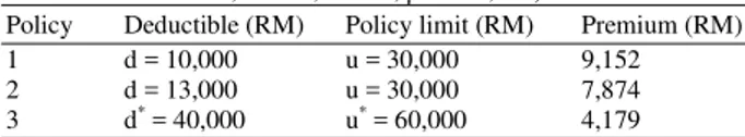
Table 4 summarizes the results of 1,000 simulations for three alternative policies, assuming that the aggregate losses follows a compound Poisson-Pareto distribution with parameters λ = 30, α = 10, β = 135,000. As an example, the first policy provides a RM30,000 coverage or limit per loss above a RM10,000 retention or deductible for a premium of RM9,152. In other words, the insured retained the first RM10,000 of loss, whereas the insurer pays any amount of loss above RM10,000 up to the limit of RM30,000 (a total loss of RM40,000). The second policy is similar to the first, but with an increased deductible value. The third policy provides a RM60,000 aggregate coverage or limit above a RM40,000 aggregate retention or deductible for a premium of RM4,179. In other words, the insured retained the first RM40,000 of aggregate losses, whereas the insurer pays any amount of aggregate losses above RM40,000 up to the limit of RM60,000 (a total aggregate losses of RM100,000).
The calculation of premium is based on the assumption that the estimate of premium is equal to the expected value of claim costs obtained from simulation, plus a loading charge equivalent to the fixed expense of RM1,000 and the variable expense of 15% of expected claim cost, i.e., premium = 1.15E(Z)+1000, where Z is the random variable for claim or loss covered by the insurer.
Fig. 4: Simulated retained loss (compound Poisson-Pareto distribution, d = 10000, u = 30000)
Fig. 5: Simulated retained loss (compound Poisson-Pareto distribution, d* = 40000, u* = 60000)
Table 4: Alternative insurance policies (Poisson-Pareto compound distribution, λ = 30, α = 10, β = 135,000)
Policy Deductible (RM) Policy limit (RM) Premium (RM) 1 d = 10,000 u = 30,000 9,152 2 d = 13,000 u = 30,000 7,874 3 d* = 40,000 u* = 60,000 4,179
The simulated retained losses for policy 1 and 3 are illustrated in Fig. 4 and 5. Note that the retained losses for deductible and limit per individual loss shown in Fig. 4 is more skewed compared to the retained losses for deductible and limit per aggregate basis shown in Fig. 5. In particular, most retained losses are less than RM10,000 for policy 1 whereas for policy 3, most retained losses are less than RM20,000.
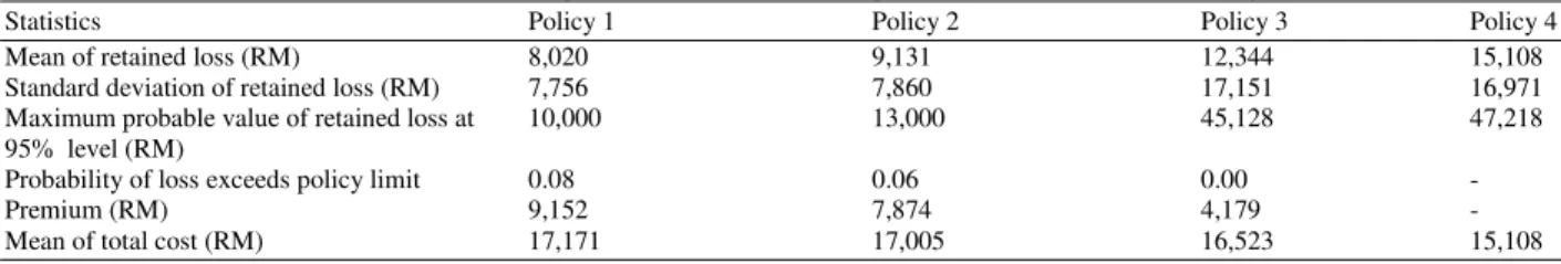
Table 5: Simulation results for alternative insurance policies (Poisson-Pareto compound distribution (λ = 30, α = 10, β = 135,000)
Statistics Policy 1 Policy 2 Policy 3 Policy 4 Mean of retained loss (RM) 8,020 9,131 12,344 15,108 Standard deviation of retained loss (RM) 7,756 7,860 17,151 16,971 Maximum probable value of retained loss at 10,000 13,000 45,128 47,218 95% level (RM)
Probability of loss exceeds policy limit 0.08 0.06 0.00 - Premium (RM) 9,152 7,874 4,179 - Mean of total cost (RM) 17,171 17,005 16,523 15,108
The fourth policy has no deductible and limit and this policy can be used as a proxy for losses without any insurance coverage.
From the insured’s perspectives, based on the maximum probable value of retained loss at ninety-five percent level and the standard deviation of retained loss, the least risky strategy is policy 1 (RM10,000 retention per loss), followed by policy 2 (RM13,000 retention per loss), policy 3 (RM40,000 retention per aggregate losses) and no insurance coverage. However, the ranking for the least expensive strategy which is based on the premium is reversed, where most savings can be made on the premium provided by policy 3, followed by policy 2 and 1.
Based on this information, an insured, which can be represented by an individual or a company, can make an informed decision on which strategy to pursue. If the insured is deciding to have additional risk reduction made possible by the RM10,000 retention per loss policy compared to the RM40,000 retention per aggregate losses policy, the insured should consider whether the additional expected total cost of RM17171-RM16523 = RM648 is worthy of the additional risk reduction.
CONCLUSION
This study approximates the compound distribution of aggregate losses using a simulation approach. In particular, the approximation of aggregate losses is based on a compound Poisson-Pareto distribution which is often a popular choice for modeling aggregate losses because of its desirable properties. Based on the results, the approximation of a compound Poisson-Pareto distribution via simulation approach agree with the theoretical mean and variance of each of the loss frequency, N, loss severity, X and aggregate losses, S. In addition to the approximation of aggregate losses, the effects of deductible and policy limit per loss and the effects of deductible and policy limit per aggregate losses are investigated. The main advantage of the simulation approach is that it allows the distributions of individual loss, aggregate losses, retained loss, aggregate retained losses, individual claim and
aggregate claims to be approximated by using a fairly straightforward simulation programming. The investigation on retained losses and insurance claims allows an insured or a company to select an insurance contract that fulfills its requirement. In particular, if a company wants to have an additional risk reduction, it can compare alternative policies by considering the worthiness of the additional expected total cost which can be estimated via simulation approach. It is also worth to note that different simulations can be run to examine the sensitivity of the results to different assumptions concerning the type and parameters of the assumed frequency and severity distributions. Finally, the simulation approach can be applied on any types of losses and disasters and may not be limited to the actuarial and insurance areas.
REFERENCES
Bickerstaff, D.R., 1972. Automobile collision deductibles and repair cost groups: The lognormal model. Proc. Casualty Actuar. Soc., 59: 68-102. http://www.casact.org/pubs/proceed/proceed72/720 68.pdf
Chaubey, Y.P., J. Garrido and S. Trudeau, 1998. On the computation of aggregate claims distributions: Some new approximations, insurance. Math. Econ., 23: 215-230. DOI: 10.1016/S0167-6687(98)00029-8 Dropkin, L.B., 1964. Size of loss distributions in Workmen’s Compensation insurance. Proc. Casualty Actuar. Soc., 51: 198-242. http://www.casact.org/pubs/proceed/proceed64/641 98.pdf
Heckman, P. and G. Meyers, 1983. The calculation of aggregate loss distributions from claim severity and claim count distributions. Proc. Casualty Actuar. Soc., 70: 22-61. http://www.casact.org /pubs/proceed/proceed83/83022.pdf
Jensen, J.L., 1991. Saddlepoint approximations to the distribution of the total claim amount in some recent risk models. Scandinavian Actuar. J., 2: 154-168.
Panjer, H., 1981. Recursive evaluation of a family of compound distributions. ASTIN Bull., 12: 22-26. http://www.actuaries.org/LIBRARY/ASTIN/vol12 no1/22.pdf
Papush, D.E., G.S. Patrik and F. Podgaits, 2001. Approximations of the aggregate loss distribution. Casualty Actuar. Soc. Forum, Winter, pp: 175-186. http://www.casact.org/pubs/forum/01wforum/01wf 175.pdf
Pentikainen, T., 1977. On the approximation of the total amount of claims. ASTIN Bull., 9: 281-289. http://www.actuaries.org/LIBRARY/ASTIN/vol9n o3/281.pdf
Seal, H., 1977. Approximations to risk theories F(X, t) by the means of the gamma distribution. ASTIN
Bull., 9: 213-218.
http://www.actuaries.org/LIBRARY/ASTIN/vol9n o1and2/213.pdf
Venter, G., 1983. Transformed beta and gamma distributions aggregate losses. Proc. Casualty
Actuar. Soc., 70: 156-193.
http://www.casact.org/pubs/proceed/proceed83/831 56.pdf