The Impact of Priority Rules on Logistic Objectives: Modeling with the Logistic Operating Curves

(1)

Abstract_{—As the logistics objectives of a production play} an increasingly significant role in an enterprise’s success, the relevance of sequencing also grows due to its ability to directly influence the objectives throughput time and schedule reliability in the production.

To solve the sequencing problem on the shop floor the priority rule tends to be used first and foremost due to its ability to find decisions quickly and to be implemented easily. Nonetheless an appropriate priority rule is usually selected based on concrete cases and requires each of these cases to be evaluated using simulations.

This paper will introduce an approach that applies the Logistic Operating Curve Theory to derive generally applicable, qualitative information regarding the impact of different priority rules as well as develop a universal, quantitative model for describing the impact of priority rules on the logistic objectives of a production. Decisions can be made without using simulations.

Index Terms_{— Logistic Operating Curves, Logistics and} Supply Chain, Production Planning and Control, Scheduling and Sequencing

I. INTRODUCTION

An enterprise with good logistics tends to grow comparatively quicker and turn higher profits than an enterprise whose logistics are less developed resulting from today’s market’s demands [1]. In order to optimally design a company’s logistics it is imperative that the production’s logistic objectives - work-in-process (WIP), utilization, throughput time and schedule reliability – are considered comprehensively [2]. Within the production process this is accomplished by production control [1], [3]. According to Lödding [1] the tasks involved in controlling Manuscript received July 13, 2009. This work was supported by the German Research Foundation within the context of the research project

Modellbasierte Bewertung der logistischen Wirkung von Prioritätsregeln in der Reihenfolgeplanung under Grant NY 4/21-1.

Wiebke Hartmann is with the Institute of Production Systems and Logistics at the Leibniz University of Hanover, An der Universitaet 2, 30823 Garbsen, Germany (phone: +49(0)511-762-19809; fax: +49(0)511-762-3814; e-mail: hartmann@ifa.uni-hannover.de).

Andreas Fischer was with the Institute of Production Systems and Logistics at the Leibniz University of Hanover. He is now with the Sennheiser GmbH & Co KG, 30900 Wedemark, Germany (e-mail: Andreas.Fischer@sennheiser.com).

Peter Nyhuis has been appointed both as a professor for Production Systems, Logistics and Work Sciences as well as the director of the Institute of Production Systems and Logistics at the Leibniz University of Hanover, An der Universitaet 2, 30823 Garbsen, Germany (e-mail: nyhuis@ifa.uni-hannover.de).

production include generating orders, releasing orders, controlling capacities and sequencing. Among these, sequencing is particularly significant because it can directly influence the logistic objectives, and, in addition to controlling capacities it is the only production control measure that can temporarily intervene in the production on short notice [1], [4]. For this reason, the following paper focuses on sequencing, exemplarily presenting the results from the German Research Foundation funded research project Using Models to Describe the Impact of the Priority Rule on Logistic Objectives.

In this paper we have chosen to focus on solutions within sequencing using the priority rule. Using the Logistic Operating Curves Theory developed by Nyhuis [5], the goal is to universally describe the effects of different priority rules, thus allowing them to be compared. Based on the results enterprises will be able to select the sequencing rule best suited to the respective operating situation with minimal effort and thus ensure that the targets are frequently attained. The procedure will be described in the following using the influence of priority rules on the logistic objective throughput time as an example.

II. SEQUENCING METHODS

Numerous problem solving methods which can also be used for sequencing orders have been developed in the past [6]. The first which are to be mentioned here are optimization methods, which, as the name implies, aim to determine the optimum for an objective function. Enumeration methods such as Linear Programming, Branch and Bound as well as dynamic programming are typical of these.

Since the early 1980s, new methods and problem solving algorithms have been combined with artificial intelligence (AI) to determine efficient solutions. These methods are based on emulating the rules humans use for perceiving and understanding; common examples include expert or agent systems as well as neural networks and fuzzy logic.

In addition to the mentioned approaches there are also conventional heuristics and priority rules. With both of these problem solving methods, finding an optimum solution is consciously refrained from. Instead the methods aim to quickly determine a qualitatively sufficient resolution. A more detailed presentation of these methods would exceed the scope of this paper, however, extensive

The Impact of Priority Rules on Logistic

Objectives: Modeling with the Logistic

Operating Curves

(2)

descriptions of the methods can be found in [7]-[14]. In order to decide which method should be used to subject sequencing to a universal modeling within the mentioned research project, the procedures were evaluated based on the quality of their solutions, the effort required to find a solution as well as their practical relevance. Their short computing times and easy implementation are the reasons why priority rules have established themselves on the shop floor despite their solutions being of lower quality than those methods that aim for the optimal solution [15]. There are local, global, simple, composite, static and dynamic priority rules. Simple and local (workstation specific) rules are mainly applied because they are robust against disruptions e.g., in the production system, are more transparent and can be used to make decisions onsite i.e., near where the process is actually occurring [15]-[17]. For this reason, we have chosen to focus on these priority rules in this paper, too. The most frequently discussed simple, local priority rules are the First-in-First-out rule (FIFO) which triggers the orders in the sequence that they arrive at the workstation, the throughput dependent priority rules shortest processing time (SPT) and longest processing time (LPT), and finally, the slack time rule (ST) which prioritizes orders with the least remaining inter-operation time until they are completed. For a definition of the throughput time components see [5]. Priority rules that optimize setup times will not be addressed here, since the examples here centre on analyzing the Throughput Time Operating Curve (TTOC) and priority rules that optimize setup times generate a TTOC that approximates the Throughput Time Operating Curve for the FIFO rule which has already been comprehensively described by Nyhuis [5].

III. MODELING

Although sequencing using priority rules is a relatively well researched area, please refer to [4] for an extensive discussion, the authors of these studies have yet to reach any generally applicable conclusion about the impact of priority rules. There are three reasons for the to some extent contradicting research and development results: First the majority of studies conducted up to now cannot be compared with one another because they are based on different operating situations i.e., different production data, output rate data, production programs etc. A further reason is that the validity of many studies is limited because they focus on only one of the logistic objectives. Frequently only the output rate data are compared with one another, whereas, further parameters such as the corresponding WIP levels which can differ although the output rates are the same, are ignored. Moreover, most of the studies conducted up until now demonstrate a lack of transparency because they have not published the assumptions and boundary conditions they are based on. This applies especially to simulations and the skeleton data they use when researching priority rules.

Consequently, up until now there has been no qualitative or quantitative model that universally reproduces the impact of the priority rules and with sufficient precision. Currently the selection of an

appropriate priority rule is oriented on concrete application cases in the respective enterprises and always requires each of the cases to be evaluated simulatively. Numerous scholars thus support the further fundamental and systematic research on the impact of priority rules which is the subject of this paper [18]-[21].

The modeling in the mentioned research project focuses on the production’s logistic objectives WIP, utilization, throughput time and schedule reliability. For the design of the model, a combined approach is pursued. First the effects of the mentioned priority rules are qualitatively mapped on the logistic objectives with the aid of simulations. The goal here is to obtain generally applicable, qualitative information for comparable operating states. The results are subsequently used to develop or further develop a mathematical impact model based on Nyhuis’ Logistic Operating Curves Theory [5]. Within the Logistic Operating Curves Theory universal correlations for the logistic objectives when applying the FIFO rule have already been formulated in a mathematical model. It thus seems obvious to use the Logistic Operating Curves as a basis for the modeling and to extend the universal correlations to include the application of other priority rules. Moreover, Nyhuis’ Logistic Operating Curves Theory is a deductive-experimental modeling approach which combines the advantages of both of the other common approaches for modeling interdependencies between the logistic objectives of a production system i.e., simulation and queuing theory. The Logistic Operating Curves Theory is suitable for formulating universal descriptions with a high level of quality whereas requiring minimal input data. This has been proven in numerous publications documenting the successful implementation of Logistic Operating Curves on the shop floor [22], [23].

The Logistic Operating Curves consist of diagrams depicting the Output Rate, Throughput Time and often Range Operating Curves together as a function of the mean WIP [5]. This paper will introduce the procedure for deriving a Throughput Time Operating Curve which describes the impact of a selected priority rule. The Throughput Time Operating Curve was selected because the Output Rate Operating Curve and Range Operating Curve are independent of the implemented priority rule when the setup time optimizing sequencing rules are neglected (see above) [5].

A. Simulation

(3)

Order of Arrival Order of Processing Production System 4 3 2 4 FIFO rule 4 3 2 4 SPT rule

4 3 2

4

LPT rule 4 3

2 4

: operation time [SCD] x

TOP: operation time

TIO: inter-operation time

TTPm: mean throughput time

FIFO 0 3 3+4 3+4+2 3 4 2 4 TIO [SCD] TOP [SCD]

TTPm= 8,00 SCD

SPT 0 2 2+3 2+3+4 2 3 4 4 TIO [SCD] TOP [SCD]

TTPm= 7,25 SCD

LPT 0 4 4+4 4+4+3 4 4 3 2 TIO [SCD] TOP [SCD]

TTPm= 9,00 SCD

Order of Arrival Order of Processing Production System

4 3 2 4 FIFO rule 4 3 2 4 SPT rule

4 3 2

4

LPT rule 4 3

2 4

Order of Arrival Order of Processing Production System

4 3

2

4 2 4 3

4 FIFO rule 4 3 2 4 SPT rule

4 3 2

4 LPT rule 4 3 2 4 FIFO rule 4 3 2

4 2 4 3

4

SPT rule

4 3 2

4 4 3 2

4

LPT rule 4 3

2 3 4 4

2 4

TOP: operation time

x TOP: operation time

TTPm= 8,00 SCD

TTPm= 7,25 SCD

TTPm= 9,00 SCD

TTPm= 8,00 SCD

TTPm= 7,25 SCD

TTPm= 9,00 SCD

Fig. 1: Impact of the priority rules on the mean throughput time

are always dealing with mean values unless otherwise noted.

In order to clarify the principle dependency of the throughput time on the priority rules, a production system consisting of one workstation and a buffer is modeled. Four orders with different work content (measured by the required operation time) enter into the workstation. At the time of the orders’ input, the workstation is free and all orders enter at the same point in time. The mean throughput times (TTPm) that result when applying the

priority rules discussed most in research i.e., FIFO, SPT and LPT are presented in Fig. 1 (unit=SCD: shop calendar days). It can be seen that dependent on the priority rule, different values for the mean throughput times ensue. The SPT and LPT rules impact the mean throughput time of a production system the most because the operation times (TOP) of the preceding orders are allocated to the following orders as inter-operation time (TIO). Evidence supporting this assessment can be found in numerous studies, see [24], [25].

The throughput time (TTP) of an order is determined by the sum of the inter-operation time and the operation time of an order. If the transport time is neglected (the transport time is usually clearly shorter than other portions of the throughput time [26] and is thus considered negligible here) the inter-operation time of an order results from the sum of the operation times of the orders processed before it. The following equation thus results for the mean throughput time: ( ) ( )⎟ ⎠ ⎞ ⎜ ⎝ ⎛ ₊ ₋ = ⎟ ⎠ ⎞ ⎜ ⎝ ⎛ ₊ =

∑

= = = = n 1 i i n 1 i i n 1 i i n 1 i i

m TOP TOP n 1

n 1 TIO TOP n 1

TTP (1)

where n represents the number of queued orders.

In Fig. 1 and (1) it can be seen that the number of queued orders influences the impact of the priority rules discussed here. Furthermore, the structure of the operation

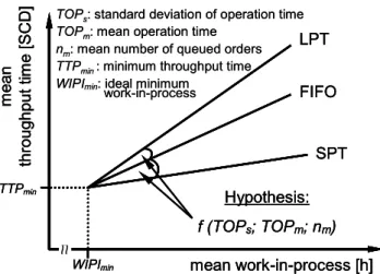
time (its mean and standard deviation) in particular affects the impact of the priority rules. With the extreme and opposing impact of the SPT and LPT sequencing rules (see above) there is a speculation that the Throughput Time Operating Curves corresponding to SPT and LPT may span a corridor within which the Throughput Time Operating Curves for all of the other priority rules might lay. The throughput time would probably then be dependent on the number of queued orders as well as the structure of the operation time. This correlation is explained in Fig. 2. In doing so, the throughput time in the proportional zone of the operating curve is examined, beyond which there is a defined minimum WIP, see [5].

The hypothesis formulates a functional correlation between the Throughput Time Operating Curves of the different priority rules which is dependent on the mean number of queued orders of a workstation (nm), the mean

operation time (TOPm) and the standard deviation of the

operation time (TOPs). The correlations in Fig. 2 apply to a

defined operating point for the workstation. If a universally applicable equation can be established for the Throughput Time Operating Curves for the SPT and LPT sequencing rules, then equations for other sequencing rules can be derived by changing the parameterization.

Once the possible impact of the priority rules has been estimated and brought together in a functional context, the influence of the mentioned parameters on the mean throughput time is examined and where applicable the identified correlations are analyzed using simulations. Details about building the simulation model as well as conducting simulations with the corresponding boundary conditions can be gained from [4].

The results of the simulation runs (with full criteria experimental design) aimed at verifying the impact of the different priority rules on the mean throughput time and the number of queued orders are depicted in Fig. 3. While one parameter is changed between different simulations the others are kept constant. This static framework assures that the results of different simulation runs can be compared. The operation time and standard deviation of the operation time were kept constant with the values TOPm = 0.4 SCD and TOPs = 0.3 SCD.

mean work-in-process [h]

me a n thr oug hput ti m e [SCD] TTPmin SPT FIFO LPT Hypothesis:

f (TOPs; TOPm; nm)

WIPImin

TOPs: standard deviation of operation time

TOP_m: mean operation time

n_m: mean number of queued orders

TTPmin: minimum throughput time

WIPImin: ideal minimum

work-in-process

mean work-in-process [h]

WIPImin mean work-in-process [h]

WIPImin

TOP_m: mean operation time

n_m: mean number of queued orders

TTPmin: minimum throughput time

WIPImin: ideal minimum

work-in-process

Fig. 2: Dependency of the priority rules’ influence on the TTPm –

(4)

WIPm[h] 0 20 40 60 80

0 60 100 160

LPT

FIFO SPT

TTPm[SCD] _nm_[-]

WIPm[h] 0

80 160

0 60 100 160

TTPm: mean throughput time nm: mean number of queued orders

WIPm: mean work-in-process : simulation points

LPT FIFO SPT WIPm[h] 0 20 40 60 80

0 60 100 160

LPT

FIFO SPT

TTPm[SCD] _nm_[-]

WIPm[h] 0

80 160

0 60 100 160

TTPm: mean throughput time nm: mean number of queued orders

WIPm: mean work-in-process : simulation points

LPT

FIFO SPT

Fig. 3: Impact of priority rules on the mean throughput time and number of queued orders – Simulation results

The results reflect the impact of the priority rules as was already hypothetically assumed. The corridor formed by the SPT and LPT priority rules is clearly recognizable. The linear correlation of the two parameters TTPm and nm over

WIPm further implies that there is also a direct correlation

between these two parameters. This correlation was already identified in the 1960s and formulated as Little’s Law. It states that the quotient from the mean throughput time and the mean number of queued orders of a production system is constant as long as the operating situations are comparable [27]. The following correlation can be derived:

LPT , m LPT , m FIFO , m FIFO , m SPT , m SPT , m n TTP n TTP n TTP =

= (2)

The significance of this law for deriving a mathematic equation for the priority rule-dependent throughput time will become clearer later in this paper.

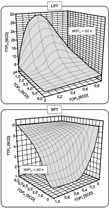
Additional simulations were conducted in order to examine how the structure of the operating time (TOPs and

TOPm) impacts nm and thus TTPm. The results are shown in

Fig. 4, please refer to [4] for an extensive discussion. The three dimensional profile depicted in Fig. 4 results after superimposing simulation runs with different operating states with a mean WIP of 60 hours.

With the 3D-profile the impact of the SPT and LPT rules on the mean throughput time is first universally mapped.

B. Mathematical Modeling

The results from simulation are used in the following to also describe the throughput time quantitatively. The aim is to establish a system of equations with which the mean throughput time of each priority rule can be quantitatively described through simple parameterization.

The procedure for quantitatively describing the impact will be briefly presented here, further details may be gleaned however from [4]. Based on the knowledge about the extreme behavior of the LTP and SPT priority rules (see Fig. 3) a basic equation for the Throughput Time Operating Curves is determined. Subsequently, the impact of the mean and standard deviation of the operating time is integrated into it.

The starting point for developing the basic equation is (2) (Little’s Law). According to it, the Throughput Time

TOPm: mean operation time TTPm: mean throughput time

WIPm: mean work-in-processnm: mean number of queued orders

1 2 3 4 5 6 TT Pm [SC D ] 6,0 5,0 4,0 3,0 2,0 1,0 0 TO_P m [SC

D] _1,0 0,8

0,6 0,4

0,2 0

TOPs

[SCD]

WIPm= 60 h

SPT 32 28 24 20 16 12 8 4 TTP m [S C D ] 0 1,0 2,0 3,0 4,0 5,0 6,0 TO_P m [S_C D_] 0 0,2 0,4 0,6 0,8

TOPs[SCD ]

WIPm= 60 h

LPT

TOPm: mean operation time TTPm: mean throughput time

WIPm: mean work-in-processnm: mean number of queued orders

1 2 3 4 5 6 TT Pm [SC D ] 6,0 5,0 4,0 3,0 2,0 1,0 0 TO_P m [SC

D] _1,0 0,8

0,6 0,4

0,2 0

TOPs

[SCD]

WIPm= 60 h

SPT 1 2 3 4 5 6 TT Pm [SC D ] 6,0 5,0 4,0 3,0 2,0 1,0 0 TO_P m [SC

D] _1,0 0,8

0,6 0,4

0,2 0

TOPs

[SCD]

WIPm= 60 h

1 2 3 4 5 6 TT Pm [SC D ] 6,0 5,0 4,0 3,0 2,0 1,0 0 TO_P m [SC

D] _1,0 0,8

0,6 0,4

0,2 0

TOPs

[SCD]

WIPm= 60 h

SPT 32 28 24 20 16 12 8 4 TTP m [S C D ] 0 1,0 2,0 3,0 4,0 5,0 6,0 TO_P m [S_C D_] 0 0,2 0,4 0,6 0,8

TOPs[SCD ]

WIPm= 60 h

LPT 32 28 24 20 16 12 8 4 TTP m [S C D ] 0 1,0 2,0 3,0 4,0 5,0 6,0 TO_P m [S_C D_] 0 0,2 0,4 0,6 0,8

TOPs[SCD ]

WIPm= 60 h

32 28 24 20 16 12 8 4 TTP m [S C D ] 0 1,0 2,0 3,0 4,0 5,0 6,0 TO_P m [S_C D_] 0 0,2 0,4 0,6 0,8

TOPs[SCD ]

WIPm= 60 h

LPT

Fig. 4: Impact of the SPT and LPT priority rules on the mean throughput time depending on the structure of the operating time (mean and standard deviation)

Operating Curve for a priority rule can be determined as:

FIFO , m FIFO , m x , m x , m TTP n n

TTP = ⋅ (3)

The equation for the Throughput Time Operating Curve of the FIFO rule has been known since Nyhuis [5]. How to determine the first factor of the equation is explained in the following using the example of the SPT rule.

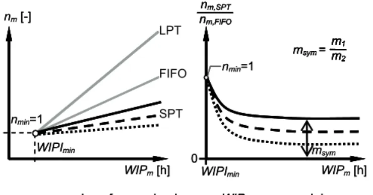
Fig. 5 depicts the correlation garnered from the simulation runs and presented in Fig. 3 as well as the curve for the quotient of the mean number of queued orders for both the SPT and FIFO rules as the relevant part of (3).

Mathematically, the function for the quotient from the equations of two straight lines can be expressed as:

2 m 2 1 m 1 FIFO , m SPT , m b WIP m b WIP m n n + ⋅ + ⋅

= (4)

(5)

WIPm[h] nm[-]

nmin=1

WIPImin

LPT

SPT

FIFO nmin=1

nm,SPT nm,FIFO

WIPm[h] WIPImin

0

: variation of the structure of the operation time

n_m: mean number of queued orders WIP_m: mean work-in-process

WIPImin: ideal minimum work-in-process

n_min: ideal minimum number of queued

orders

msym m1 m2 msym=

WIPm[h] nm[-]

nmin=1

WIPImin

LPT

SPT

FIFO nmin=1

nm,SPT nm,FIFO nm,SPT nm,FIFO

WIPm[h] WIPImin

0

: variation of the structure of the operation time

orders

: variation of the structure of the operation time : variation of the structure

of the operation time

orders

msym m1 m2 msym=

m1 m2 m1 m2 msym=

Fig. 5: Identifying a basic equation

lines [28]. If the structure of the operating time (i.e., TOPm

and TOPs) is varied, it can be seen that the quotient tends

toward different limits. This is influenced mathematically by the factor referred to as the asymptote value msym calculated from the quotient of m1 and m2, see Fig. 5. In

order to parameterize msym the least squares method is

used. Least squares is a standard method used in fitting curves [28]. First a suitable type of function is determined with which the results from the simulation for msym can be

depicted. In this case, power functions are the most suitable for approximating the values of the simulation results. As a result and after reducing the parameters using the least squares method once more, the following correlation for the SPT priority rule is established (see also [4]):

( )

( TOPv)

TOPv F

d d m m

⋅ ⋅

= ₂_.₂₅

1 1 1

2 1

65 . 1

(5) In (5) the coefficient of variation for the operation time

TOPv is used to describe the quotient of TOPs and TOPm

(i.e., the common mathematical definition of the coefficient of variation). From the simulation results and the identification of the corresponding type of function, it turns out that d1 and F1 are characterized respectively by a

straight line and a power function and thus can be integrated into the asymptote equation. The following correlations then result:

(10 TOP ) 0.75

1 1

F ; 4 . 5 TOP 175 . 0

d ₁_.₇

m m

1=− ⋅ + = _⋅ − ₊

(6) Finally, the values for b1 and b2 of the basic equation

have to be determined. In order to do this, the correlations from Fig. 5 are once again considered. If the WIP value in the extreme case equals the ideal minimum work-in-process (WIPImin), then all of the equations take

on the value 1. Mathematically this is only possible when b1 = b2. Using the least squares method the constant b1 can

now be determined based on the simulation data. For the SPT rule, the resulting value is 14.

After the basic equation is completely parameterized for the SPT rule, the mathematical equation for the mean throughput time of the priority rule SPT can be formulated as:

( )( )

FIFO m m

m TOPv

m

TOPv TOPm

m

SPT

m TTP

WIP

WIP TOP

TOP

TTP _,

25 . 2

75 . 0 10

1

,

14

14 4

. 5 175

. 0

4 . 5 175

.

0 1.7 1.65

⋅ +

+ ⋅ ⎟ ⎟ ⎟

⎠ ⎞

⎜ ⎜ ⎜

⎝ ⎛

+ ⋅ −

=

⋅ ⋅ ⎟ ⎟ ⎠ ⎞ ⎜

⎜ ⎝ ⎛

+

⋅ −

(7) Similarly for the Throughput Time Operating Curve of

the LPT rule the following correlation results:

( )( )

FIFO , m

m TOPv

25 . 2 m

TOPv 75 . 0 TOPm 10

1 m

m LPT

,

m TTP

5 WIP 8

. 5 TOP 175 . 0

8 . 5 TTP 175 . 0

5 WIP TTP

65 . 1 0 . 2

⋅

+ ⋅ ⎟ ⎟ ⎟

⎠ ⎞

⎜ ⎜ ⎜

⎝ ⎛

+ ⋅ −

+ =

⋅ ⋅⎟⎟ ⎠ ⎞ ⎜⎜

⎝ ⎛

+

⋅ −

(8) With all of the equations it is important to keep in mind

that the units need to be neglected, since the least squares method only offers the optimal numeric solution. This is not unusual since equations for models are often developed without including the units for the sake of clarity, see [29].

In order to ensure that the identified equation describes the behavior of a real workstation with sufficient quality, the quality of the depiction of (7) and (8) needs to be evaluated. This is accomplished in two steps: first the deviation of the calculated throughput time from the simulated throughput time is analyzed and then the shape of the distribution for the identified deviations. The deviation of the calculated values from the simulated values is determined with the help of the mean and quadratic relative deviation (DRELm and DRELq) as

standard parameters of a descriptive statistic [28].

The distribution shape of the deviations is analyzed using the so-called χ2

-Test or Chi-Squared Test. This is required to ensure that there are no significant individual deviations. As anticipated there are few deviations and the Logistic Operating Curves are almost parallel with one another with a WIP level considered to be comparable to one in the practice (a WIP range considered to be relevant to the practice is up to 15-times the WIPImin).

Even when the values particularly with the quadratic relative deviation are over 10% further evaluations show that the deviations between the calculated and simulated values for the throughput time – both for the LPT as well as the SPT rule – are less than 20% with a probability of approximately 90%. Moreover, it can be proven with the χ2

-Test that there are no significant individual deviations (for a more exact derivation of these results see [4]).

The primary aim of the work in the aforementioned research project was to derive a generally applicable correlation for describing the impact of priority rules on the logistic objectives of a production. It was shown that the impact of the priority rules on the mean throughput time can be quantitatively described in the form of Logistic Operating Curves. Within this context and considering the entire model is dependent on only two parameters which are influenced by the priority rules, some loss of quality in the mapping is absolutely permissible.

(6)

and 12.15% for DRELq – are even better than those for the

LPT and SPT rules. It could also be proven with the χ2

-Test that there were no significant individual deviations between the simulated and calculated values.

IV. SUMMARY

This paper presented an approach for universally and quantitatively describing the impact of priority rules on the production’s logistic objectives with the aid of Logistic Operating Curves to avoid simulations in future. As an example the procedure for the production’s logistic objective throughput time was presented. Based on the simulation results for qualitatively describing the impact of various priority rules, a mathematical modeling of its depictions was undertaken with the aid of Nyhuis’ Logistic Operating Curve Theory which quality has been evaluated. It could be proven that with a balance between a high quality depiction and a high level of transparency a universal description of the throughput time is possible with the developed mathematical model. It is possible to formulate both qualitative and quantitative statements about the impact of the priority rules. Thus, a method is now available which eliminates the (previously) existing lack of a generally applicable model for the priority rules’ impact on the production’s logistic objectives. In the future it is possible to select priority rules without having to implement a comprehensive simulation for a specific operating state on a workstation. Furthermore, there are numerous application possibilities: The Throughput Time Operating Curves that are determined can for example be drawn upon to evaluate production process or implemented in order to provide support for planning activities.

In order to orient the research results of future project work even more closely on the practice, the impact of disruptions need to be integrated into the modeling which has up until now been developed assuming ideal conditions. Thus for example, the assumption that the selected priority rule will be strictly maintained is an idealized assumption that is often not the case on the shop floor e.g., due to rush orders. Moreover, additional research is needed regarding the modeling of other priority rules which prioritize for example, completion dates or optimizing setup times. The research project will also be focusing on deriving generally applicable information about other logistic objectives for the production, such as the schedule reliability, and integrating it in a mathematical model since, up until now the correlations from Yu’s Schedule Reliability Operating Curve have only been applicable when the FIFO rule has been in place [30].

REFERENCES

[1] H. Lödding, Verfahren der Fertigungssteuerung. 2nd ed., Berlin et al.: Springer-Verlag, 2008. (English translation to be published in 2010.)

[2] H.-P. Wiendahl, P. Nyhuis, A. Fischer, D. Grabe, „Controlling in Lieferketten“ in G. Schuh (Ed.),

Produktionsplanung und -steuerung, 3rd ed., Berlin et al.: Springer-Verlag, 2006, pp. 467-510.

[3] H.-P. Wiendahl, Fertigungsregelung. München et al.: Hanser-Verlag, 1997.

[4] A. Fischer, Modellbasierte Wirkbeschreibung von Prioritätsregeln. Garbsen: PZH-Verlag, 2007.

[5] P. Nyhuis, H.-P. Wiendahl, Fundamentals of production logistics: theory, tools and applications. Berlin et al.: Springer-Verlag, 2009.

[6] K. Evers, Simulationsgestützte Belegungsplanung in der Multiressourcen-Montage. Hannover: Universität Hannover, 2002. [7] G. Zäpfel, Produktionswirtschaft - Operatives

Produktions-Management. Berlin, New York: Gruyter-Verlag, 1982.

[8] O. Schrödel, Flexible Werkstattsteuerung mit objektorientierten Softwarestrukturen. München: Hanser-Verlag, 1992.

[9] S. F. Smith, “Knowledge-based production management: approaches, results and prospects” in Production Planning & Control, 3rd ed. vol. 4, 1992, pp. 350-380.

[10] A. Daub, Ablaufplanung. Bergisch Gladbach, Köln: Josef Eul-Verlag, 1994.

[11] J. Sauer, “Knowledge-based systems in scheduling” in T. L. Leondes (Ed.), Knowledge-based systems techniques and applications, San Diego: Academic Press, 2000, pp. 1295-1325. [12] J. Schultz, P. Mertens, „Untersuchung wissensbasierter

und weiterer ausgewählter Ansätze zur Unterstützung der Produktionsfeinplanung - ein Methodenvergleich“ in

Wirtschaftsinformatik, 42nd ed. vol. 1, 2000, pp. 56-65.

[13] H.-J. Zimmermann, Operations Research: Methoden und Modelle für Wirtschaftsingenieure, Betriebswirte, Informatiker. 2nd ed., Wiesbaden: Vieweg-Verlag, 2008.

[14] S. S. Rao, Engineering optimization: theory and practice. New York et al.: Wiley-Verlag, 2009.

[15] R. Schulz, Parallele und verteilte Simulation bei der Steuerung komplexer Produktionssysteme. Ilmenau: TU Ilmenau, 2002.

[16] S. R. Lawrence, E. C. Sewell, “Heuristic, optimal, static, and dynamic schedules when processing times are uncertain” in

Journal of Operations Management, 15th ed. vol. 1, 1997, pp. 71-82.

[17] R. Vahrenkamp, Produktionsmanagement. 6th ed., München: Oldenbourg-Verlag, 2008.

[18] V. Portougal, D. J. Robb, “Production scheduling theory: just where is it applicable” in Interfaces - International journal of the Institute for Operations Research and the Management Sciences, 30th ed. vol. 6, 2000, pp. 64-76.

[19] J. N. D. Gupta, “An excursion in scheduling theory: an overview of scheduling research in the twentieth century” in

Production Planning & Control, 13th ed. vol. 2, 2002, pp. 105-116. [20] K. McKay, M. Pinedo, S. Webster, “Practice-focused

research issues for scheduling systems” in Production and Operations Management, 11th ed. vol. 2, 2002, pp. 249-258. [21] K. Kemppainen, Priority scheduling revisited – Dominant

rules, open protocols and integrated order management. Helsinki: Helsinki School of Economics-Verlag, 2005.

[22] P. Nyhuis, “Practical applications of logistic operating curves” in Annals of the CIRP, 56th ed. vol. 1, 2007, pp. 483-486. [23] P. Nyhuis, G. von Cieminski, A. Fischer, “Applying

simulation and analytical models for logistic performance prediction” in Annals of the CIRP, 54th ed. vol. 1, 2005, pp. 417-422.

[24] J. H. Blackstone, D. T. Phillips, G. L. Hogg, “A state-of-the-art survey of dispatching rules for manufacturing job shop operations” in International Journal of Production Research, 20th ed. vol. 1, 1982, pp. 27-45.

[25] R. Conway, W. Maxwell, L. Miller, Theory of Scheduling. New York: Dover Publications, 2003.

[26] H.-P. Wiendahl, Betriebsorganisation für Ingenieure. 5th ed., München et al.: Hanser-Verlag, 2005.

[27] J. D. C. Little, “A proof of the queueing formula L = λ W” in Operations Research, 9th ed. vol. 3, 1961, pp. 383-387. [28] I. N. Bronstein, K. A. Semendjajew, G. Musiol, H. Mühlig,

Taschenbuch der Mathematik. 7th ed., Frankfurt am Main: Harri Deutsch-Verlag, 2008.

[29] H.-J. Bungartz, S. Zimmer, M. Buchholz, D. Pflüger,