.... .,...FUNDAÇAo . .... GETULIO VARGAS
Sf\lJ"\
\1~I()SDL PI ""'(.l1 1....,.\
LC()\()\IIC \
~
. .
EPGE
Escola de Pós-Graduaçao em Economia
The Effects of the MinintulIl Wage
on Earnings and Entployment in
Brazil
"
Pro:F.
Sara
Lemos
&\
j/
(University College London-
ucb--.-./
LOCAI.
Fundação Getulio Vargas
Praia de Botafogo, 190 - 100 andar - Auditório
DATA
02103/2000 (58 feira)
HORÁRIO
16:00h
The Effects ofthe Minimum Wage on Earnings and
Employment in Brazil
Sara Lemos!
March, 2000
ABSTRACT
This paper analyzes the effects of the mlmmum wage on both, eammgs and
employment, using a Brazilian rotating panel data (Pesquisa Mensal do Emprego - PME)
which has a similar design to the US Current Population Survey (CPS). First an intuitive
description of the data is done by graphical analysis. In particular, Kemel densities are used
to show that an increase in the minimum wage compresses the eamings distribution. This
graphical analysis is then forrnalized by descriptive models. This is followed by a discussion
on identification and endogeneity that leads to the respecification of the model. Second,
models for employment are estimated, using an interesting decomposition that makes it
possible to separate out the effects of an increase in the minimum wage on number of hours
and on posts of jobs. The main result is that an increase in the minimum wage was found to
compress the eamings distribution, with a moderately small effect on the leveI of
employment, contributing to alleviate inequality.
1. INTRODUCTION
Employment and eamings are two important macroeconomic variables in capitalist
societies. To increase the leveI of these variables is always among the aims of the
Govemment. One institutional variable that can be used by the Govemment to influence
eamings and employment is the minimum wage. The possibility of using the minimum wage
as an instrument of macroeconomic policy immediately asks for its effects on employment
and eammgs. The direction and magnitude of this effect - the elastícíty - provides the
quantitative and qualitative ínformatíon to the questíon of the effects of the minimum wage on
the leveI ofboth, employment and eamings. The knowledge ofthese elastícities might enable
the Govemment to use the minimum wage as an instrument of macroeconomic policy against
poverty, ínequality and unemployment.2
The aím of thís paper is to estímate these elastícítíes. Theír expected directíons and
magnitudes are as follows. On one hand, the elasticity of the minimum wage with respect to
the other wages/eamíngs is expected to be positive because workers bargain to maintain their
relative wages. However, its magnitude is expected to vary across the eamings distributíon,
once the minimum wage is expected to have stronger impact on the lower tail of the
distribution. This is because different occupations compare their wages to the wages of
different reference groups. And different groups do not react identícally in presence of a
minimum wage increase (Grossman, 1983).
Thus, we can expect different elasticities for different percentiles of the eammgs
distribution. An increase in the minimum wage would affect the eamings distribution in two
ways: a) shifting the distribution to the right, pushing its mean up, and b) changing the shape
of the distribution, because of the change in its variance. The change in its variance is due to
the different elasticities across the distribution. As higher elasticities are expected in lower
percentiles, the change in íts variance is such that the distribution becomes less disperse. Thís
change in the shape of the eamings distribution would ímply a nonparallel shift of the
distribution to the right.3 Other things equal, this shift is expected to reduce inequality.
On the other hand, there ís no consensus about the direction of the elastícity of the
employment wíth respect to the minímum wage, whích might be eíther negatíve or
nonnegative. The standard neoc1assical model predicts a negative e1asticíty if the minimum
2 See Dinardo, Fortin and Lemieux (1994) and Card and Krueger (1995) for issues on the effect of the
rninimum wage on inequality. Or see the original article of Stigler (1946).
3 The following figure illustrates what is meant by nonparallel shift of the distribution to the right:
•
- _ _ _ _ _ _ _ _ _ _ _ _ _ _ _ _ _ _ _ _ _ _ _ _ _ _ _ _ _ _ _ _ _ _ _ _ _ 1
wage is fixed above the leveI of the equilibrium wage in a perfect competitive labour market
(if fixed at the exact equilibrium leveI or below, it does not have any effect). This is because
in order to afford higher wages employers would have to lay off some workers. This theory is
supported by empirical evidence showing that "a 10% increase in the minimum wage reduces
teenage employment by one to three percent" (Brown etc. aU, 1982, p.524). An update of
Brown's et aI. survey by Wellington (1991), conc1udes that the employment effects of the
minimum wage are negative but small: 10% increase in the minimum wage would lower
teenage employment by 0.06 percentage points. More recently, Deere et aI. (1995), Kim and
Taylor (1995) and Neumark and Wescher (1995) also found negative effects. However, new
empirical evidence, which still needs stronger theoretical support, has found nonnegative
elasticities (Card, 1992a and 1992b; Katz and Krueger, 1992; Machin and Manning, 1993;
Card Katz and Krueger, 1994; Card and Krueger, 1994, 1995 and 1998; Bernstein and
Schmitt, 1998 and Dickens et aI., 1999). A minimum wage increase needs not reduce
employment, and might increase it if the wages are lower than the productivity of workers.
This could happen in a monopsonistic model4, where firms are paying wages below the
marginal productivity ofthe worker (Dickens et aI, 1999; Dickens et aI, 1995c).
It is important to notice that employment is going to be affected not only because of
the change in the minimum wage itself, but also because ofthe changes in the wages/earnings,
via changes in the minimum wage. In other words, employment can be thought of as being a
function of both, the minimum wage and wages/earnings. And wages/earnings, as being a
function of the minimum wage: N
=
f[mw, w(mw)]. Thus, the aim here is to estimate thereduced form ofthis as yet unidentified structural modeI.
Given the nature of the relationship between these variables, the goal of
macroeconomic policy is to change the shape of the wage/earnings distribution but not to
destroy jobs. If the elasticity of the other wages with respect to the minimum wage and the
elasticity of employment with respect to the minimum wage have opposite signs, the
Governrnent might have to decide among two compromising goals: increasing the leveI of
4 This model is attractive because it is general enough to allow the minimum wage to have either a negative or a
nonnegative effect on employment. It is also attractive because: 1) it can explain the existence of a spike in the
empirical earnings distribution; 2) it distinguishes between the elasticity of labour supply to an individual frrm
• 'I.
,
employment or increasing the leveI of wages. On the other hand, if both elasticities are
positive, or positive and nonnegative respectively, an increase in the minimum wage is likely
to be desirable. In the case where an increase in the minimum wage has nonnegative or no
significant effect on employment, its effects on inequality will strongly depend on its effects
on the shape ofthe earnings distribution. If the employment elasticity is zero, this can be used
as an identifying restriction to identify the effect of the minimum wage on inequality, as in
Dinardo et aI (1996). If the employment elasticity is negative, it is still possible to study the
effects of the minimum wage on inequality, but then an exerci se of calibration is required, to
take into account the negative impact on employment. 5
Thus, this paper is going to estimate the effect of the mlnImum wage on both,
employment and earnings. It is organized as follows. The second section afier this
introduction presents the data. Section 3 is a descriptive section, which first describes the
behaviour of the minimum wage, setting it into context in Brazil (section 3.1), and then
presents some descriptive statistics (section 3.2) and descriptive models (section 3.3). Section
4 discusses identification and endogeneity and estimates the earnings model (section 4.1) and
the employment mo deIs (section 4.2). Section 5 conc1udes.
2. DATA
This paper analyses the effects ofthe minimum wage in Brazil, using Brazilian data to
estimate the earnings and employment elasticities. The data used is a rotating panel data for
Brazil called PME (Monthly Employment Survey) which has a similar design to the US CPS
(Current Population Survey). From 1982 to 1998, PME interviewed over 8 million people
across the six main Brazilian metropolitan regions: Bahia (BA), Pernambuco (PE), Rio de
which different frrrns in the same market are differentially affected by the rninimum wage (Dickens Machin and Manning, 1994 and 1999) .
5 It is Important not to forget that the effects of the minimum wage on inequality depend also on who earns
the minimum wage (see Card and Krueger, 1995).
Furthermore, in any case, the speed and the magnitude ofthe increase play an important role. For example, a more desirable effect on the leveI of employment, in case of wages lower than the marginal product, rnight be reached with a policy that combines successive small increases instead of one single large increase, that could lead to lay offs (see Card and Krueger, 1995; Dickens, Machin and Manning, 1997; and Machin and Manning, 1994, 1996). Thus, a rninimum wage increase program should suggest a schedule of time and optimal percentages to maximize the employment and the effects against inequality and poverty, as well as mechanisrns to enforce and monitor it.
•
'I'.
,
-Janeiro (RJ), Sao Paulo (SP), Minas Gerais (MG) and Rio Grande do Sul (RS). Its monthly
periodicity is essential for the analysis of the Brazilian labour market because wages
bargaining during the sample period occurred yearly, bi-yearly, quarterly and even monthly,
depending on the leveI of the inflation rate and stabilization plan in vigor.
Each metropolitan region is composed of towns and cities, divided into Census
sectors. PME first selects sectors and then households within sectors. The selection of
households in the sectors is conducted with probability proportional to the number of
households in every sector. This is so to guarantee random sampling, once the probability of
selection of each household within a metropolitan region is constant regardless of the size of
the city/town where the household is located (IBGE, 1983).
Then a panel is defined as a set of households divided into four subsets, PI, P2, P3,
P4. A second and a third panel of the same length are selected, without coincident
households, and also divided into four subsets (QI, Q2, Q3, Q4 and RI, R2, R3, R4). The
rotating scheme substitutes one of the subsets of the panel every month. That is, in month
t+I, panels PI, P2, P3, P4 started offin month t, are substituted by PI, P2, P3, Q4. In month
t+2, panels PI, P2, P3, Q4 are substituted by PI, P2, Q3, Q4. And so on, in such a way that in
the 13th month, panels PI P2 P3 P4 are back in the survey before they are definitely
excluded6. In this fashion, it is guaranteed that a) 75% of the households will be common to
6 The following table illustrates the rotating panels scheme:
~ear/month week
1988 1 2 3 4
May P1 P2 P3 P4
June P1 P2 P3 04
Ju/y P1 P2 03 04
August P1 02 03 04
September 01 02 03 04
October 01 02 03 R4
November 01 02 R3 R4
December 01 R2 R3 R4
1989
January R1 R2 R3 R4
February R1 R2 R3 P4
March R1 R2 P3 P4
April R1 P2 P3 P4
..
"
.
\•
every two consecutive months 7, and b) that every couple of years 100% of the sample is
repeated. This scheme allows not only monthly and yearly comparisons, but also seasonal
comparisons (IBGE, 1983).
According to the above scheme, every household is interviewed for 4 consecutive
months, is out of the survey for 8 consecutive months, and is again interviewed for another 4
consecutive months, when is then definitely exc1uded from the survey. That is, within a
period of 16 months, a household is interviewed 8 times (IBGE, 1991)8. From the household
selected, around 20% ofthe sample is dropped for non-response. From the remaining sample,
around 50% were interviewed 4 times consecutively and around 13% were interviewed eight
times consecutively, on average across metropolitan regions.
At a more detailed leveI, it is important to remember that PME is a household, not an
individual survey. There is no guarantee that the same individuallives in the same household
for 16 consecutive months; or that the same individual, within a household, answers all the
interviews. But some controls alIow for checking whether the survey is folIowing the same
individual over time. After differencing eamings, around 25% of the data for the whole
period is lost, on average, across metropolitan regions. This is because individuaIs which are
not followed for subsequent months are dropped. An individual could not be observed for a
subsequent month either because he lost his job (or because he never had a job in the survey
period) or because of the rotating panel scheme (two observations are lost, rather than one,
because the individual is not observed for 8 consecutive months, but for 4 and 4, with 8
months interval in between.9
Comparisons of demographics and economics across regions indicate that the data
does not show selectivity bias in any direction. AIso, comparisons of demographics and
economics between people interviewed four and eight times show no bias.10
7 Although conceptually 75% of the households should always be common to two consecutive months,
practical problems provoked twice the break of the flow. 1) In August of 1988 the sample of PME was
reduced by 20%, excluding Census sectors and households within Census sectors. 2) In October of 1993,
because ofthe new Census, a new sample for the PME was selected. From October of 1993 to January of 1994 this new sample was slowly implemented. Thus the panels of January of 1994 are 100% different
fiom the ones of January 1993. A part fiom this two big changes, whenever the selection of new panels in
a particular sector was exhausted, the sector was substituted. AIso, the impossibility of interviews in areas
of extreme violence lead to the substitution ofhouseholds within Census sectors.
8 For a detailed description ofthe data, see IBGE (1983) and (1991).
9 The same differencing, considering the three breaks in the panels above mentioned, keeps respectively
around 77%, 75% and 73% ofthe data, on average, across metropolitan regions.
10 For a detailed analysis on selectivity bias and non-response attrition on PME, see Neri (1996).
..
..
To deflate nominal variables in the PME, the deflator chosen was INPCII (National
Consumers Price Index), calculated by IBGE (Brazilian Institute of Statistics and Geography),
the same institution that conduces PME. This index was desegregated at regional leveIs, so
that the regional data could be deflated by regional deflators. This was an attempt to reduce
measurement error likely to arise from the deflation of nominal data in a high inflationary
environrnent disregarding regional inflation rate variations. 12
Finally, the data on the minimum wage was obtained from the Brazilian Labour Ministry.
3. DESCRIPTIVE ANAL YSIS
3.1 MINIMUM WAGE AS MACROECONOMIC POLICY IN BRAZIL
As mentioned above, the main motivation for the study of the effects of the minimum
wage on both employment and earnings is the possibility of its use as social macroeconomic
policy against inequality poverty and unemployment. But that is not the only role played by
the minimum wage in Brazil. The minimum wage can be regarded as the cost of a production
input (labour) [either as the cost of a minimum wage worker or as affecting the cost of
workers earning more than one minimum wage (workers higher up in the earnings
distribution), as discussed in the introduction], and therefore, it can affeet prices. Beeause of
this, the minimum wage can be used as stabilisation macroeeonomie policy against inflation
(Camargo, 1984; and Macedo and Garcia, 1978). This is particularly true if the minimum
wage assumes a role of indexor, as happened in Brazil in the last few decades. In sueh high
inflationary environrnent, with distorted relative priees, agents took the offieial increases in
the minimum wage as a signal for their bargain on prices and wages/eamings. Carneiro and
Faria (1998) argue that with the introduetion of the first official wage macroeconomie poliey
II The choice of the deflator and the deflation method are very important in a high inflationary process
context such as the one experienced in Brazil in the last 20 years. The inflation rate from O 1.1982 to
09.1998 was 5,338,550,750,980%. To see more about the issues evolved in deflation of wages in presence of high inflation, see Neri (1995). AIso see discussion on the choice among INPC versus IPCA (Wide Consumer Price Index) on a forthcorning paper on the effects of the rninimum wage on eamings and employment in presence ofhigh and low inflation.
12Because the INPC is centered on the 15th ofthe month, and the wages are usually paid at the beginning of
the month, a geometric mean of two subsequent months was used as an attempt to center the INPC on the
. - - - -
-•
.,
•
in the 60's, the minimum wage was used not only as stabilisation policy but also as
co-ordinator ofthe wage policy.
Thus the minimum wage was altematively used as social or stabilisation
macroeconomic policy in Brazil. The choice depended a) on whether the Govemment was
populist or conservative, b) on the leveI of inflation; and c) on the bargain power of the
workers at every point in time. The more populist the Govemment, the lower the inflation
and the stronger the bargaining power of workers, the more the minimum wage tended to be
used as social rather than as stabilisation policy.
A1though a proper discussion of the role of the minimum wage in Brazil is far beyond
the scope of this paper13, it might be instructive to briefly pIace the minimum wage into
context in the Brazilian economy. The minimum wage was first introduced in 1940 as a
social policy. Its leveI was such as to provide the minimum diet, transport, clothing and
hygiene for an adult worker. The price of this minimum basket was different across the
country, such that there was 14 different leveIs for the minimum wage, with the highest leveIs
for the Southwest (SE) and the lowest for the Northwest (NE) (Foguel, 1997). Wells (1983,
p. 305) believes that the initial leveIs of the minimum wage were "generous relative to
existing standards" once about 60 to 70% of workers earned below these initiallevels. On the
other hand, Saboia (1984) and Oliveira (1981) believe that the minimum wage did not rise but
rather legitimated the low wages of the unskilled.
Although the minimum wage was set to buy a minimum basket, most often this did
not seem to be a worry when adjusting its nominal value. Roughly, the evolution of the real
minimum wage was: a) a dramatic decrease from 1940 to 1951; b) a steep increase from 1952
to 1961; c) a decrease from 1962 to 1974; d) an increase from 1974 to 1979 and stabilisation
until 1982; e) a decreasing tendency, oscillating with the different stabilisation plans, from
1983 onwards ..
The real minimum wage decreased dramatically during the 40's because its nominal
value was not adjusted between 1943 and 1952, while the inflation was around 160%,
combination which lead the minimum wage to reach its lowest leveI ever. On the other hand,
the combination of the economic boom during the 50's, the high productivity, the strong
unions and the social-populist govemments, in a favourable environrnent for increasing
13 For a detailed description ofrnacroeconornic policy in Brazil, see Abreu (1992).
..
..
wages, lead the minimum wage to reach its highest leveI ever. In the following years (from
1962 unti11974) wages decreased, and so did the minimum wage, as a result ofthe recession
combined with rising inflation and rather defensive than stronger unions (Singer, 1975). The
minimum wage then was 40% lower than in the 50's. In its early existence the real minimum
wage was used as a social policy whose leveI was strongly associated with the aItemance of
populist and conservative govemments (Velloso, 1988 and Bacha, 1979). This role changed
when the dictatorship Govemment installed in 1964 associated the high inflation with
increases in the wages. Thus, a recessive wage macroeconomic policy was implemented,
whose one of the main strategy was to control the increases in the minimum wage (Macedo
and Garcia, 1978), with nominal minimum wage adjustments below the inflation. The
minimum wage was transformed "from a social policy designed to protect the worker's living
standard into an instrument for stabilisation policy (Camargo, 1984, p.19).
The boom in the late 60's increased wages, however by much less than the increase in
productivity (Foguel, 1997). This increase was not accompanied by an increase in the
minimum wage, which remained stable. In a more favourable environment, and also due to
the pressure of accelerating inflation, the leveI of the real minimum wage was preserved from
1974 until 1979, with yearly adjustments just about right to compensate the inflation. In
1979, the wage policy changed substantially. Bi-year1y adjustments of 110% of the inflation
were given to workers who earned in the range of 1 to 3 minimum wages. Lower percentual
of adjustment were given as the range of eamings was higher up in the earnings distribution.
Soon the minimum wage became an indexor for all kinds of contracts. This policy lead the
economy to superindexation. And even afier its use as indexor was forbidden by law in 1987,
the minimum wage continued playing a major role in prices and wages/earnings bargaining.
With the inflation back in the early 80's, the priorities of the macroeconomic policy
were essentially combating the inflation. Several stabilisation plans, orthodox and the most
heterodox ones, lead to a series of different wages policy. The minimum wage continued
being used as a component of the wage macroeconomic poIicy even afier the end of the
dictatorship regime in 1985, with some sporadic and unsuccessful attempts to use it as a social
poIicy. The importance of the minimum wage was not onIy because of the indexation of the
the minimum wage.14 Because of this, the leveI of the minimum wage had an impact on the
Govemment's budget. This impact combined with the fiscal crisis did not allow the
govemment to give more generous adjustments to the minimum wage.
In 1983 the percentual of increase of wages of workers earning in the range of 1 to 3
minimum wages went down to 100% rather than the previous 110% ofthe inflation. In 1984
the minimum wage became national. The different leveIs across the country had slowly been
converging to a national leveI over previous years. In 1988 the new Constitution (afier the
military regime) fixed the national minimum wage by law as to provi de the minimum diet,
accommodation, education, health, leisure, c1othing, hygiene, transport, and retirement to an
adult worker and his family.
From 1986 to 1994 the minimum wage was systematically decreased, due most1y to
the persistency of high levels of inflation. The minimum wage suffered two major decreases
in 1983 and 1987 (Reis, 1989), despite of the attempt of 15% increase by Plano Cruzado, in
February of 1986, frustrated by the acceleration ofthe inflation (Velloso, 1988). Under Plano
Cruzado, alI wages should be increased automatically whenever the accumulated inflation
was higher than 20%. The minimum wage was adjusted twice according to this rule, but still,
by the implementation ofPlano Bresser, in June of 1987, the minimum wage was 25% lower
than in March of 1986. Under Plano Bresser, wages should be frozen for 3 months and then
monthly indexed by past inflation. The monthly indexation preserved the leveI of the real
minimum wage from September of 1987 until the implementation ofPlano Verao, in January
of 1989, when prices were again frozen. From May of 1989 onwards the minimum wage was
14 Carneiro and Henley (1998) argue that the minimum wage became less important as a coordination
instrument in the 80's and that its effect in the long run on the real wages became less and less important. But this is not a new debate in Brazil. The 1970 Populational Census showed an increase in inequality in the country. Tms increase in inequality was associated with the systematic decreases in the minimum wage since 1940, and in particular, after the 1964 recessive wage macroeconornic policy. The minimum wage was identified as deterrnining the evolution ofwages (Souza and Baltar, 1980; Wells, 1983; and Saboia 1983), although some would disagree on that (Macedo and Garcia, 1978). But even though Macedo e Garcia (1979) tried to minimize the role of institutional variables, and in particular the role of the minimum wage, on the increase in inequality, specially for the SE, where the demand for labour increased, they afrrm that the unimportance of the minimum wage in the NE was not so evident.
Attempts to explain the effect ofthe minimum wage on wages/earnings were made in a neoclassical and structuralist framework [se e structural theories ofCEPAL (Cornission for the Development of Latin America), of University of Campinas (SP, Brazil), and in particular, see Souza (1980a, 1980b) and Tavares (1975 adnd 1985)], as well as using Lewis' theory ofthe subsistence wage (Lewis, 1954). Not only the association ofthe minimum wage with inequality was extensively discussed in Brazil, but aIs o the association of decreasing minimum wage, signalizing decreasing wages, driving a
•
adjusted monthly, what once more preserved its real value at the leveI of the beginning of
Plano Verao. However, the dramatic acceleration of the inflation in the beginning of 1990,
just before Plano Collor, was responsible for a big fall in the minimum wage. Under Plano
Collor, initially no systematic rules for indexation were announced, strategy which had to be
abandoned because the inflation could not be maintained at low leveIs. Another big falI
followed from non adjustment of the nominal minimum from March to May of 1990. From
then on the minimum was adjusted monthly until February of 1991. Once more the non
adjustment of the nominal minimum wage, combined with 65% inflation from March until
August of 1991 induced another big fall. In September 1991, the indexation was restricted to
workers who earned in the range of 1 and 3 minimum wages. The minimum wage was
adjusted quarterly until December of 1992. In 1993 the minimum wage was adjusted
bi-monthly until J une and then bi-monthly, as the inflation was persistent. In March of 1994 a daily
indexor for prices and wages was introduced as prelude for the Plano Real implemented in
July of 1994. In September of 1994 the minimum wage was adjusted and was then frozen
until April of 1995, which induced a fall in its real value once the inflation was not null in the
period. In May of 1995, with the inflation stabilised, the minimum wage was increased by
42%. Since then the minimum wage has been yearIy adjusted, with low but not null inflation.
Under Plano Real, with the stabilisation of the inflation, the minimum wage has not been used
explicit1y as stabilisation policy.
Table 3.1 and graph 3.1a summarize the behaviour of the real minimum wage from
1982 until 1998 (period for which the data for this paper is available). Before the first
stabilization plan (Cruzado Plan, February of 1986) the nominal minimum wage was adjusted
every 6 months (May and November). From then on, it was erratically adjusted, depending
on the current adjustment rules of successive stabilization plans (Cruzado Plan lI, June of
1986; Bresser Plan, June of 1987; Verao Plan, January of 1989; Verao Plan lI, May of 1989;
Collor Plan, March of 1990; Collor Plan lI, January of 1991; and Real Plan, July of 1994).
Under the Real Plan, the adjustments became yearly (May). The highest leveI of the real
minimum wage, within the period, according to table 3.1, was in November of 1982
(R$255.06), before the acceleration ofthe inflation. Its value decreased continuously, during
-
.-a long period ofhigh infl.-ation, re.-aching its lowest leveI in August of 1991 (R$82,21). It then
presented a positive tendency followed by a large single decrease when the Real Plan was
implemented15. At that time, it was fluctuating around R$100,0016, and, since then, its
nominal value has been increased in about 5 to 12% per year.
3.2 DESCRIPTIVE STATISTICS
The behaviour of real variables is mainly influenced by the inflation in the period.
The high inflation, combined with nominal earnings adjustments lower than the inflation,
induced: 1) large decreases in the real minimum wage; 2) high variation in both, real
earnings and real minimum wage.
The behaviour of the real minimum wage in the period is shown in table 3.1 for the
whole country and in graph 3.1, for the whole country and per regions. The highest leveI of
the real minimum wage is in SP, where the leveI of inflation is the lowest. On the other hand,
the lowest leveI of the real minimum wage and highest leveI of inflation are in PE and BA.
More generally, the real minimum wage is higher, and the inflation rate is lower in Southeast
(SE) [RJ, SP and MG] and South (S) [RS], than in Northeast (NE) [BA and PE]. Although
the leveI of the real minimum wage differs, its pattem of behaviour is very similar across
regions (see graph 3.1).
The variation in the real earnings and real minimum wage for each region and for the
whole country over time, are shown in graph 3.2. The pattem ofthe behaviour ofreal average
earnings is very similar in all regions and it is also similar to the behaviour of the minimum
wage. PE presents the smoothest pattem and the lowest leveI of real earnings, while SP
presents the most variable pattem and the highest leveI. Another way to look at the variation
in real eamings as compared with variation in the real minimum wage is to look at what
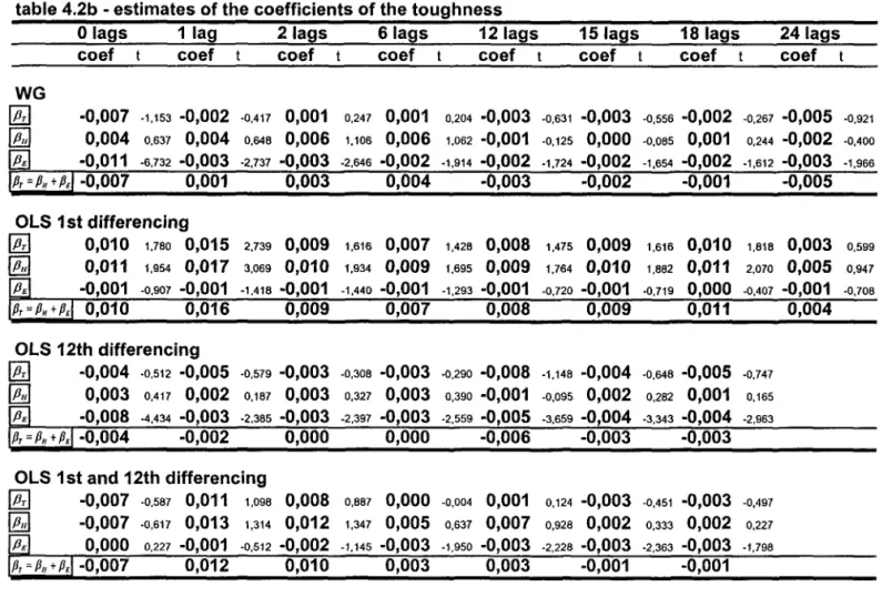
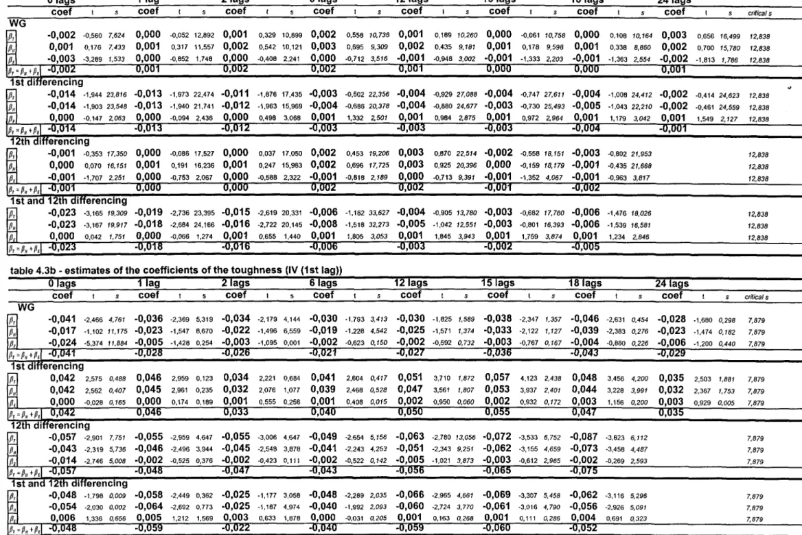
Machin and Manning (1994) call "toughness" ofthe minimum wage. Toughness is defined as
the ratio of the real minimum wage and the real average earnings, which is the key variable in
15 At that time there was two currencies in the country: Cruzeiros Reais and URV (Real). The inflation
measured in Cruzeiros Reais was much higher than the inflation measured in Reais, as it was the idea
behind the plano Although the IBGE published the inflation measured in Reais in July of 1994, in this
paper this rate was corrected (in 21.99%) for the inflation in Cruzeiros Reais in July of 1994.
16 The real minirnum wage and earnings values in this paper are in Reais of December of 1997. When the
Real plan was implemented, the nominal value of the minimum wage was around R$70,00, which in terrns of Reais of December of 1997 is R$100,00. (The exchange rate of Reais to US dollars was one to one
when the Real Plan was implemented, and it was approxirnately 1,70, in September 1999).
",
-
.-many minimum wage studies (Brown et aI., 1982). This measure is shown in table 3.1 and
graphed in graph 3.3, also for every region and for the whole country over time. Again, the
partem is very similar in all regions. Now SP presents the smoothest partem and the lowest
leveI, and PE the most variable partem and the highest leveI. All these figures show a similar
partem of variation in both, real minimum wage and real eamings, suggesting that both
variables can be related. It also shows high variation in the real minimum wage, what
contributes for the efficiency ofthe estimators discussed below.
While the toughness shows how the minimum wage and the mean of the earnings
distribution are associated, a more complete and informative picture is given by analyzing the
association of the minimum wage with various percentiles of the eamings distribution. Graph
3.4 shows the 5th, 10th, 50t\ 90th, 95th percentiles and the mean ofthe eamings distribution for
the whole country, as well as ratios ofthe 90-10,90-50 and 10-50 percentiles. This is to show
that the partem of the 10th percentiles of the eamings distribution are similar to the partem of
the minimum wage in graph 3.1. Graph 3.5 shows the partem of the 10th percentile of
earnings distribution for the whole country and per region. This resemblance is not that
strong for percentiles higher up in the distribution. This is shown numerically in table 3.2 that
shows the correlations between the real minimum wage and the percentiles and mean of the
eamings distribution for every region. These correlations confirm the graphical analysis
(graphs 3.4 and 3.5) that the minimum wage is more strongly correlated with lower than with
higher percentiles of the eamings distribution. It also shows that the correlations between the
minimum wage and the 10th percentile are stronger in NE than in SP. Important to note that
the minimum wage is expected to impact more poor than rich regions. In particular, changes
in the minimum wage are expected to induce a bigger change in eamings of poor (NE) than of
rich regions (SE and S, in particular, SP). Thus, the conceptual question here is how changes
in the minimum wage changes eamings, that is, how the changes of variables are related,
rather than their relation in leveIs. That is the economic reason why specifications in
first-differences are chosen over specifications in leveIs.
Graphs 3.4g to 3.4i also show ratios ofthe percentiles ofthe earnings distributions for
the whole country. The partem of the ratio of the 10th to 50th percentiles (graph 3.4i) is
roughly negative and then positive, which is the same partem of the real minimum wage in
·
-,
-
.-percentiles and the behaviour ofthe minimum wage (graphs 3.4i and 3.1). This resemblance
is reassuring of the correlation between the minimum wage and the 10th percentile of the
eamings distribution showed above. The ratios ofthe percentiles 90th to 10th (graph 3.4g) has
the opposite pattem. Both set of ratios, 50th to 10th and 90th to lOt\ together, being a measure
of inequality, suggest that inequalíty increased and then decreased over the sample period.
Another way to measure inequality is to look at the growth rate of different percentiles
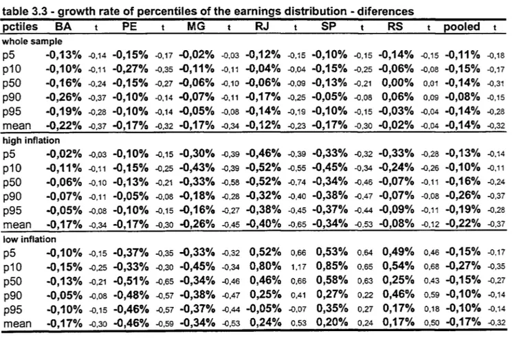
ofthe eamings distribution. Table 3.3 shows the average eamings growth rate per month for
the mean and 5t\ 10th, 50th, 90t\ 95th percentiles for the whole country and for every region.17
The average eamings growth rate over the whole sample period is negative for most
percentiles in all regions. This is probably due to over three decades of high inflation. An
evidence of the influence of high inflation on eamings growth is given when the sample
period is split into high (04.82 to 08.94) and low (09.94 to 09.98) inflation periods. That is,
before and after Real Plano In presence of high inflation, inequality seems to have risen, with
eamings decreasing at a higher rate at the bottom than at the top of the distribution for all
regions. Incidentally, the minimum wage had an important role in high inflation periods,
being used as an indexor and as stabilization policy, as mentioned in section 3.1. In low
inflation, inequality seems to have decreased. The negative growth rates for all regions
observed in the high inflation period turned into positive for RJ, SP and RS in the low
inflation period. This is reassuring of the percentile ratios figures above, which show that
inequality increased and then decreased over the sample period. The figures on growth rate of
percentiles also suggest that inequality is increasing across regions, with NE becoming
relatively poorer. Not only NE is becoming relatively poorer, but it also presents the highest
leveIs of inequality across the country. This is shown in table 3.4, by the Gini coefficient,
which is a standard measure of inequality. This coefficient does not change much when the
whole sample period is split between high and low inflation periods.
The above figures, particularly a) the higher correlation of the minimum wage with
lower percentiles of the eamings distribution; b) the resemblance in the tendencies of the
minimum wage and the ratios of percentiles; c) the raise in inequality in presence of high
17 This is done by regressing the various percentiles and the mean of the earnings distribution on a trend, or,
altematively, the differences of the percentiles and the mean of the earnings distribution on a constant.
Although many of the coefficients were not significant in the specification in differences, it was still
14
-..
-
.-inflation coinciding with the largest decreases on the minimum wage; d) the higher correlation
of minimum wage and earnings in NE than in SE associated with higher inequality in NE than
in SE; suggest that the minimum wage might play a role in explaining some of the inequality
in the period.
A measure of the bite of the minimum wage is the percentage of people earning one
minimum wage, namely "spike".18 Table 3.1 shows that the spike varies roughly between 2%
and 9% for the whole country.19 But from the above pieces of evidence, the biggest spikes in
the earnings distribution are expected to be in the NE, and the smallest ones in SP. That is
because the minimum wage is expected to impact more poor than rich regions. For the very
same increase in the minimum wage, more people are expected to be affected in a poor than
in a rich region. That is what graphs 3.6 and 3.7 to 3.9 show, reassuring the above figures on
correlation. Graph 3.6 shows the evolution of the size of the spike over time for every region
and for the whole country. And graphs 3.7 to 3.9 show the actual spike in the distribution of
eamings for one particular year of high inflation, 1992, for the whole country, PE and SP20.
The verticalline (which is in some cases completely covered by the spike) is the value ofthe
minimum wage in every month. Graphs 3.6, 3.8 and 3.9 show that the spikes in NE are
bigger than in SE and S and that they are particularly small in SP for the whole period. Also,
a) the percentage of people earning a minimum wage or less and b) the percentage of people
eaming less than a minimum wage follow the same partem as the percentage of people
earning one minimum wage (spike).
preferred over the specification in leveI, because the robustness of the estimates in leveIs could be due to spurius association. Anyhow, the pattems, either in leveIs or in differences, do not differ substantially.
18 Because of rounding approxirnations, more precisely, spik:e is defmed as the percentage of people
eaming in the range [( -O.02MW + MW) ~ earnings ~ (+O.02MW + MW)].
19 From March to June of 1994, there is no a punctual minimum wage. This is because the minimum wage
was fixed in 64.79 URV, but paid in Cruzeiros Reais, which was the official currency in the country. The value of the rninimum wage in Cruzeiros Reais depended upon the day of payment, because the value of the UR V was daily adjusted according to the daily inflation in Cruzeiros Reais.
In the literature, the minimum wage (MW,) is usually converted in Cruzeiros Reais by the URV of the last day of the month (month,). However, in this fashion, the spike can not be captured, once the MWt is usually paid at the beginning ofmontht+h rather than at the last day ofmontht. Thus, in this paper, MWt is converted in Cruzeiros Reais by the average URV ofthe frrst 7 days ofmontht+1• The average ofthe frrst 7
days of the montht+1 was chosen because, by law, the payment of the MWt must be done at the latest at the 5th working day ofmontht+1 (CLT, art. 459, law 7855/89).
..
•
...
..
.
-Conceming the size of the spike and average eamings, PE has the highest spike and
the lowest average eamings and SP has the lowest spike and the highest average eamings (see
graphs 3.6 and 3.2). Both, the size ofthe spike and the value ofthe real minimum wage affect
the average wage. First, the more people eaming the minimum wage, the bigger the spike,
and the smaller the average eamings. Average eamings are lower, the higher the spike,
because the mean is influenced by the mass in the spike, which is in the lower tail of the
distribution. Second, the lower the leveI of the real minimum wage the lower the average
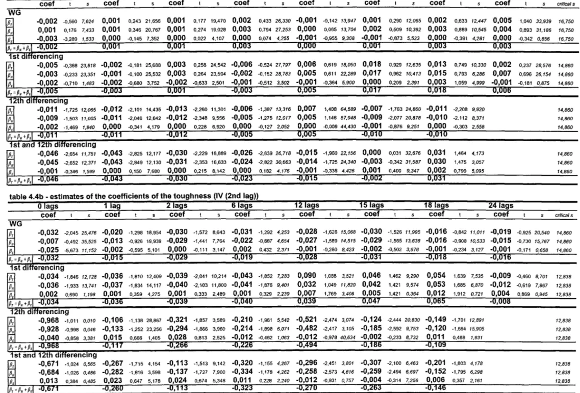
eamings. This shows that the minimum wage is tough. Table 3.1 shows how the size of the
spike reacts to increases in the minimum wage, as well as the reaction ofthe toughness. Note
in particular, that in August of 1991, when the minimum wage reached its lowest leveI within
the period, spike jumps from 1.02% to 6.07%, and toughness jumps from 11.11 % to 23.35%.
Regarding toughness as a measure of inequality, a positive and strong correlation between
spike and toughness suggests that the bigger the spike, the higher the inequality. That is what
table 3.5 shows.
Graphs 3.10 to 3.12 show the Kemel estimation of the eamings distribution for the
whole country and for PE and SP for a particular year of high inflation, 1992. These graphs
show the eamings distribution before and after an increase in the minimum wage. In 1992,
according to table 3.1, the minimum wage was increased every fourth month: January, May
and September of 1992 and again in January of 1993. Graphs 3.10d,h,1 to 3. 12d,h,1 show the
change in the shape of the distribution after every adjustment in the minimum wage. The
eamings distribution becomes less disperse due to changes in the lower tail. This nonparallel
shift to the right of the distribution of eamings is an evidence of the effect of an increase in
the minimum wage on eamings.
In fact, in the remaining months, when there is no increase in the minimum wage, the
distribution becomes more disperse. This happens because when the nominal minimum wage
is not increased, but the inflation is high, it is as if the real minimum wage was actual1y
decreased. And if an increase in the minimum wage shifts the distribution of eamings
nonparallely to the right, a decreased is expected to shift it to the left. In years of low
inflation, for example, a non increase in the nominal minimum wage does not shift the
distribution to the left. This is what graphs 3.13 to 3.15 show. These graphs show the Kemel
estimation of the eamings distribution for the whole country and for PE and SP for a
'"
-".
-
.-particular year oflow inflation, 198421• In 1984, according to table 3.1, the minimum wage
was increased every sixth month: May and November. Graphs 3.l3d, j to 3.15d, j show the
change in the shape of the distribution after every adjustment in the minimum wage. Again,
the eamings distribution becomes less disperse due to changes on the lower taiL But in the
remaining months of 1984, when there is no increase in the nominal minimum wage and the
inflation is yet not so high such as to "induce" a decrease in the real minimum wage, the
distribution does not shift to the left.
The Kemel estimation of the eamings distributions present this pattem of behaviour
over the whole sample period, what is a reassuring evidence that the minimum wage affeets
eamings. It is also a reassuring evidence that the minimum wage has a higher impact on
poorer than on richer regions. The behaviour of the Kemel densities is in line with the above
analysis.
3.3 DESCRIPTIVE MODELS
As a counterpart of the graphical Kemel estimation of the earnings distribution, a very
descriptive model was estimated. The simplest descriptive model of eamings as a function of
the minimum wage is:
lrearnit
=
a + f3lrmwt + uit ' i = 1, .. ,8millions, t=
1, ... ,169where, lrearnit is the logarithm ofreal eamings for individual i in time period t and lrmwt is
the logarithm of real minimum wage on time period t common to alI individuaIs. The month
data goes from May of 1984, to May of 1998, adding up to 169 time periods.
Let the following model be the aggregated version of the above model. Aggregating
by time period and per region:
-lrearnrt
=
a + f3lrmwrt + Urt, r=
1, .. ,6, t=
1, ... ,169where I rearnrt is the mean ofthe logarithm ofreal eamings of a11 individuaIs in region r in
time period t, and lrmwrt is the logarithm of the real minimum wage in region r in time
...
..
-
.-the real minimum wage varies across regions because .-the data was deflated with regional
deflators, which themselves vary across regions.22
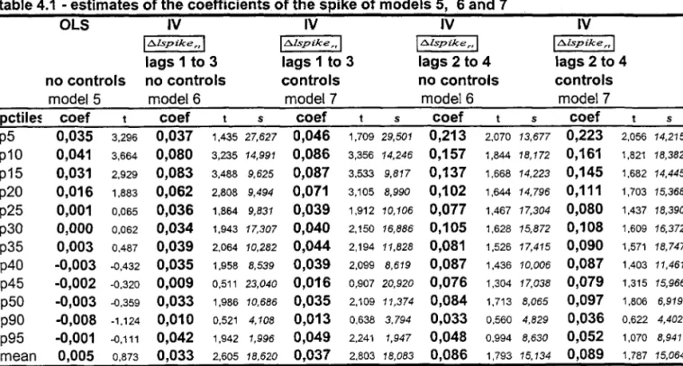
This aggregation is done not only for the mean, but also for the 5th, 10th, 15th, 20th,
25t\ 30th, 35t\ 40th, 45th, 50th (median), 90t\ 95th percentiles of the earnings distribution. In
this fashion, a more complete picture of the effect of the minimum wage on eamings is
obtained. That is because not only the effect of the minimum wage on the mean of the
earnings distribution can be estimated, but also the effect of the minimum wage on various
points across the distribution can be estimated (Dickens et aI., 1999).
Month and year dummies were added up to the specification. The month dummies try
to capture seasonal effects, while the year dummies try to capture common macro shocks
(productivity shocks, for example) allowing for them to be different every year. AIso,
stabilization plan dummies were added up to the specification, as an attempt to capture
common macro shocks under each stabilization plano As mentioned above, the whole period
can be divided into six subperiods according to the five stabilization plans plus an early period
with no stabilization plano Each of these stabilization plans had very particular roles, specially
the most heterodox ones. In Cruzado plan, for example, the prices were frozen by law; in
Collor Plan, the savings were confiscated, etc.23 Thus, these macro shocks were probably
similar within and very different across plans (the behaviour of prices, taxes, investments,
unemployment, etc.). All these time dummies, namely year, month and stabilization plan
dummies, are included as an attempt to separate out the effect of other macro variables from
the effect of the minimum wage on eamings.24
The only macro variable which was explicitly added up to the specification is past
inflation. That is because inflation was a driving force in the economy within the period.
Almost all ofthe macroeconomic policy, including the minimum wage policy, was around the
22 See discussion on identification in section 4.1.1.
23 Again, for a detailed description ofmacroeconomic policy in Brazil, see Abreu (1992) .
24AIso a dummy for structural change was included in October 1988, when the new Constitution was
promulgated. This is because the new Cosntitution changed two main aspects ofthe number ofworking hours: a) the working week was shortened from 48 to 44 hours;
b) there was a new option of working day available in the labour market: instead of the old 8 daily hours of work (with 2 hours break for lunch), workers could now work 6 consecutive hours.
Controlling for these changes is important because of the likely effect on the average number of hours worked
and on employment rate - variables here used to measure employment - as well as on earnings. In this way, the
impact of these structural changes on average hours of work and on employment rate is not confused with a change in the minimum wage.
."
stabilization of the inflation rate at low leveIs. As showed in the previous section, inflation
strongly influenced the behaviour of real eamings and real minimum wage. Another reason to
inc1ude past inflation as a regressor is to attempt to separate out the effect of the minimum
wage from the effect of inflation. This is because, as mentioned above, the minimum wage
was used as an indexor, thus, it might be capturing the effect of inflation. By inc1uding
inflation explicitly, the coefficient of the minimum wage will be measuring that portion of the
minimum wage change which was made not merely to compensate inflation.
Thus, the model was estimated for each and all of these percentiles, for the median and
for the mean, inc1uding year, month and stabilization plan dummies, as well as past inflation:
-
-(1) lrearnrt = a + f31rmwrt + 'i..5kmonthk + 'i..r/year/ + 'i.. , mestabm + mnpcvrt-J + Urt,
k
=
1, ... ,12, 1= 1, ... ,15, m = 1, .... ,6The unrestricted version of this pooled mo deI, where all the coefficients are allowed to
differ across regions, is:
-
-(2) lrearnrt
=
ar + f3,lrmwrt + 'i..5rk monthk + 'i..rr/year/ + +'i..'rmestabm + 7rrinpcvrt_1 + UrtHowever, for the saroe conceptual reason why correlations (table 3.2) were computed
in changes, versions of the above mo deIs in changes are estimated. That is, once more the
interest might be on the effect of changes in the minimum wage in changes in earnings, rather
than their relationship in leveIs. This allows for analysis of the dynaroics of the eamings
distribution over time given the behaviour of the minimum wage. Additionally, differencing
reduces the variables to stationarity, avoiding spurious regression. Thus, mo deIs 3 and 4 are:
-
-(3) 111rearnrt
=
a + f3111rmwrt + 'i..5kmonthk + 'i..r/year/ + 'i.. , mestabm + mnpcvrt_1 + I1U rt,-
-(4) 111rearnrt
=
ar + f3rl11rmwrt + 'i..5rk monthk + 'i..rr/year/ + +'i..'rmestabm + 7r,inpcvrt_1 + I1U rtwhere the dummies and the constant are added up after differencing, as well as past inflation.
The constant can be seen as the base dummy rather than the trend from the model in leveis.
The structure of the errors in the above models is heteroskedastic and serially
correlated in the mo deIs in levels25. Regarding serial correlation, models 1 and 2 were
corrected for serial correlation of the errors within panels, assuming an autorregressive
process of order 1, AR(I), specific to each region. Regarding heteroskedasticity, two sources
."
the nature ofthe conditional distribution ofreal earnings, and b) at a macro/aggregated leveI,
l;earnrt is heteroskedastic because ofthe aggregation per region.
Heteroskedasticity arises from the aggregation per region because averages computed
over a larger sample size have smaller variance, even if at the lowest micro leveI (lrearnirt ),
eamings were homoskedastic. In other words, an average computed over a larger sample size
is more reliable than an average computed over a smaller sample size. Thus, if the sample
size is assumed to be proportional to the size of the regional labour market, average eamings
in bigger regions (whose sample size are larger) are more reliable than average eamings in
smaller regions (whose sample size are smaller). It follows that the appropriate correction for
the heteroskedasticity arising from the aggregation is formalized by Weighted Least Squares
(where the weights are root sample size), which gives heavier weight to more reliable
information. Incidentally, the weighting can be justified at economic grounds as well, if the
coefficient of the minimum wage in the pooled regression is regarded as an weighted average
of the regional coefficients. In this case, if once more the sample size is assumed to be
proportional to the size of the regional labour market, the weights would be capturing the
importance of each regional labour market in estimating the pooled coefficient. While
weighting takes care of the heteroskedasticity arising from the aggregation, on the top of it,
the standard errors were also White-corrected, to take care of the heteroskedasticity of
lrearnirt •
The estimates ofthe coefficients ofthe minimum wage ofmodels 1 and 2, and models
3 and 4 are, respectively, in tables 3.6a and 3.6b, and also in graph 3.16. Note that the pattem
does not change much from leveIs to differences (compare graphs 3.16a in leveIs with 3.16b
in differences). Note in particular graph 3.16c, that graphs the coefficients of the pooled
regression in leveIs and in differences. Graph 3.16d emphasizes the bigger impact of the
minimum wage on PE than on SP, as before.
The results are very reassuring of the above analysis. First1y, the minimum wage has a
stronger impact on the lower percentiles of the earnings distribution, shifting the distribution
nonparallely to the right. Dickens et. aI (1999) found the same compressing effect when
estimating a similar specification. Just as it was suggested graphically by the Kemel
25 See below for conunents on serial correlation of the errors.
20
MDIJTECA MAr,W HENRIQUE' SfMONSEJi
tllNOACÃO GETULIO VARGAS
----=---==-=-=~===---".
-..
-distribution estimation (graphs 3.10 to 3.15), this is an evidence of the effect of the minimum
wage on inequality. Roughly, an increase in the minimum wage affects the 10th percentile
almost ten times more than it affects the 90th percentile of the eamings distribution for the
whole country (see table 3.6b and graph 3.16c). Secondly, the minimum wage has a stronger
effect on the eamings distribution of NE (poor) than of SE and S, with its smallest effect for
SP (rich) (see tables 3.6 and graphs 3.16).26
The coefficients of the minimum wage are most1y significantly different from zero
being more robust: a) for lower than for higher percentiles; b) for NE than for SE and S; and
c) for the models in leveIs than for the models in differences. The coefficient of past inflation
is significant and robust, in particular, in the specification in differences. 27
The significance and robustness of the time dummies varies across regions and across
the distribution, being more robust for the pooled regression (more degrees of freedom). The
year and month dummies are mostly significant in leveIs. In differences, the year dummies
are mostly significant for 1986 to 1989 and 1994 to 1995. These are years of acceleration of
the inflation and subsequent stabilization plans (Cruzado in 1986 and Real in 1994). The
January, February, March, June, July, September and December month dummies are mostly
significant in differences, suggesting that important seasonal pattems are present. These are
months of Holidays and Camival, except for September, where important worker categories
26 Although the coefficient of the pooled regression can be regarded as an weighted average of the regional
coefficients, a poolability test for the above restricted and unrestricted models was implemented. The result is that the hypothesis that the coefficients do not differ across regions could on1y be rejected for the 10th, 15th, 20th
and 25th percentiles. As an attempt to produce a more robust poolability test, the unrestricted mode! was SP alone versus all the rernaining re!ions pooled together. Again, the hypothesis that the coefficients do not differ could only be rejected for the 10 and the 15th percentiles. That is, the data does not have enough variability to reject the poolability higher up in he distribution (as well as in the 5th percentile) ..
The null hypothesis of these poolability tests is that there is no unobserved regional effects, in other words, H
o : Ir
=
O. In fact, the above results are in line with prior expectations, because any potentialIr
in the mode! in leveIs was wiped out when the model was frrst differenced, which is the case for models 3 and 4. In other words, the regional fixed effect affects the variables in leveIs but not in differences.Note that Chow test can only be used under the assumption of errors independent and identically distributed (iid). As discussed above, !::.U ri are assumed independent. Also, the heteroskedasticity arising from
the aggregation per region was corrected by weighting the model by the regional sample size. However, the errors might not be identical, because of some heteroskedasticity still left. Thus, care should be taken when interpreting these tests, which were here reported as an attempt to justify the pooled coefficient beyond its interpretation as an average coefficient.
27 As robustness check, mode!s 1 to 4 were estimated a) using INPC rather than IPC per region, b) using
..
-
".-negotiate wages. The stabilization plan dummies are most1y significant in leveIs, except for
plan Bresser, and are mostly significant for plans Cruzado, Bresser and Verao in differences.
The constant, which can be seen as the base dummy, is significant and very robust in leveIs
and most1y significant in differences.
Summarizing, all the pieces of evidence in this descriptive section (3.1,3.2 and 3.3) of
the strong correlation between the minimum wage and the lower percentiles of the eamings
distribution suggest that the minimum wage explains some of the inequality in the period.
AIso, it suggests, as expected, that the minimum wage has a stronger effect in poorer than in
richer regions.
The above modeIs have only described a statistical relationship between eamings and
mlmmum wage. The question asked was:
if
a person is taken at a random from lhepopulation, what is his expected (predicted) earnings, given the leveI of the minimum wage?
Of more interest would be to estimate a causal relationship between eamings and minimum
wage. The question to be asked would then be:
if
the same person is taken from thepopulation (that is, with the same characteristics), knowing which region he comes from
(poor/rich region), that is, controlling for regional effects, and the minimum wage is
increased by 1 %, by how much would his earnings be increased? An attempt to answer this
question requires a discussion on identification and on endogeneity, which is presented in the
next section.
4. IDENTIFICATION AND ENDOGENEITY
4.1 EARNINGS EQUATION
4.1.1 identification
The nominal mlmmum wage In Brazil is national, not regionat.2s That is, the
minimum wage is a constant across regions and individuaIs on a given month, and therefore,
changes in the specification: the signs of the coefficients remain the same, and their magnitude is roughly the same, as well as their significance.
28 Regional minimum wages existed until April of 1984 when they turned into a national minirnum wage.
For this reason, in this paper, the period used for estimations is from May 1984 onwards. A forthcoming paper on regional minimum wages studies the advantages and disadvantages of regional minimum wages as opposed to a national minirnum wage in Brazil.
~.
it does not vary across regions. The real minimum wage varies across reglOns, though,
because the nominal (constant) minimum wage was deflated with regional deflators, which
vary across regions. This variation, however, cannot be regarded as genuine variation in the
minimum wage, but rather as artificial variation completely driven by the variation in the
deflators. Had the data been deflated by a national rather than by regional deflators, the real
minimum wage would be a constant, just like the nominal minimum wage is. In this sense,
the real minimum wage can be regarded as a constant in the identification discussion which
follows. Put differently, in the purely descriptive mo deIs of section 3.3, the variation driven
by the regional deflators does not identify
f3 .
f3
is not identified at regional leveI or over time. First, it is not identified at a regionalleveI, because there is no regional variation. Within a month, the minimum wage is a
constant, and therefore, cannot explain variations in eamings. Second, it is not identified over
time, despite of the time variation, if no restriction on time is imposed. Suppose that the
stabilization plan, month and year dummies in the mo deIs of section 3.3 were replaced by
one dummy for every time period. This would be a much less restrictive way to model the
effect of the other macro variables on earnings. Then
f3
would not be identified at alI,because of perfect multicollinearity between the 169 time period dummies and the minimum
wage.
In the mode1s of section 3.3,
f3
is only identified because the effect of the other macrovariables on earnings is modeled by the use of stabilization plan, month and year dummies.
That is,
f3
is identified ad hoc. A more restrictive way to mo deI these macro variables wouldbe by a linear trend. In this case, deviations from the linear trend would be assumed entirely
due to the effect ofthe minimum wage. Put differently, the minimum wage would be the only
macro variable affecting eamings nonlinear1y.
f3
would again be identified ad hoc, whichdoes not guarantee that the effects of the minimum wage could be distinguished from the
effects of other macro variables on eamings. That is, there is no guarantee that
f3
is capturingthe effect ofminimum wage on eamings only. Thus, to identify