Abstract—Shake flasks have been used for screening process in fermentations for a long time. The oxygen transfer rates of the fermentation media change with viscosity. The liquid distribution in hydrophilic shake flask becomes asymmetrical as the viscosity of the liquid increases. Therefore, a non-invasive optical technique has been developed to collect angular information on the shape of the liquid at different operating conditions like shaking frequency, shaking diameter, and filling volume. This technique uses light emitting diodes, a photomultiplier tube and fluorescent solution. 16 sets of optical fibers with each set comprises of 2 optical fibers arranged in certain angle of incident light between the fibers are attached at different heights of the outside wall of a shake flask. Blue lights from the light emitting diodes are switched alternately at different heights and excite the fluorescent molecules in the flask. The emission lights are then sent through the optical fibers back to the head-on photomultiplier tube. With LabVIEW program, automatic and manual mode of signal data collections from the photomultiplier tubes are available. The digital signals received and saved indicating the liquid distribution are then analyzed in MATHLAB for the shape. However, prior to the identification of the shape of the liquid distribution in shake flask, the optimizations of the signal parameters are investigated. The influences of the intensity of the light emitting diodes and the photomultiplier tube’s sensitivity level to the liquid distribution’s signal at a certain shaking frequency and at each height at a fixed filling volume are observed. Varying these parameters change the output voltages from the photomultiplier tube. However, the shapes of the liquid distributions remain the same. The varying numbers of rotations collected in reference to the mean show acceptable percentage deviations but slight sharp increases of the percentage are shown especially at the start of the bulk liquid. With the information, signals obtained and interpreted from this setup depict invaluable information on the hydrodynamic of the liquid distribution in shake flask.
Index Terms— Liquid distribution, optimization, shake flask.
I.INTRODUCTION
Liquid distribution comprises of rotating bulk liquid and
Manuscript received March 23, 2009. This work was supported in part by Aachener Verfahrenstechnik-Biochemical Engineering, RWTH Aachen University, Germany.
A. Azizan is currently with Aachener Verfahrenstechnik-Biochemical Engineering, RWTH Aachen University, Aachen, Germany, on leave from Faculty of Chemical Engineering, Universiti Teknologi MARA, Shah Alam, Malaysia (phone: +49 (0)2418028112; fax: +49 (0)2418022265; e-mail: amizon.azizan@ avt.rwth-aachen.de).
R. Voravichan is with Thai German Graduate School at King Mongkut’s University of Technology North Bangkok, Bangkok, Thailand (e-mail: [email protected]).
J. Büchs is with Aachener Verfahrenstechnik-Biochemical Engineering,
RWTH Aachen University, Aachen, Germany (e-mail:
stagnant liquid film on the wall and at the base of the shake flask. According to Higbie’s penetration theory, the gas-liquid mass transfer sensitively depends on the thickness of the thin liquid layer on the flask wall and the contact time [1], [2]. It explains that the mass transfer occurs only close to the gas-liquid interface specifically at the liquid film. Hence, this significantly contributes to the specific mass transfer area and to the maximum oxygen transfer capacity of microorganisms in fermentation. The basic hydrodynamic information representing the gas-liquid interface is still unavailable and there are still few information on the power input consumption, volumetric mass transfer coefficient and interfacial area [3]. Currently, the information on the liquid distribution including shape and thickness in shake flask is still scarce and might only be described based on fundamental understanding of fluid flow. Liquid distribution calculations and model have been introduced with the assumption of frictionless liquid giving an insight of the liquid distribution [4]. However, in reality, at different parameters during fermentations, the liquid distribution considering frictions between liquid and wall changes and influences momentum transfer area and mass transfer area in shake flask. In high viscosity solution in shake flask which is mainly shown during fermentation, the liquid distribution is also greatly influenced. Therefore, a setup is designed to determine the liquid distribution in shake flask for further understanding of the transport phenomena and hydrodynamics of the liquid in shake flask.
II. NON-INVASIVE TECHNIQUE OF LIQUID DISTRIBUTION
A. Technique
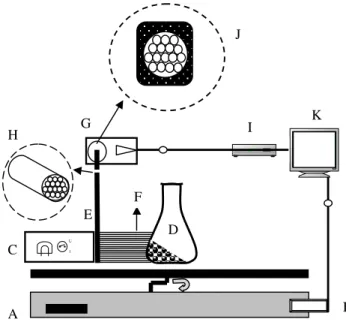
The technique involved the excitation of the fluorescent solution by a blue light from a light emitting diode (LED) at a wavelength of 480 nm. The emission light from the fluorescent was received by a compact head-on photomultiplier tube (PMT, Photosensor module H7827 Hamamatsu, Japan) at 515 nm. The technique was non-invasive having 16 sets of plastic optical fibers (POF, Conrad, Germany) positioned outside of the wall of the flask. Each set has 2 optical fibers separated by an angle degree of 45 as shown in Fig. 1.
This specific angle of fibers positioned at the wall enabled optimum light exposure close to wall detecting the coming of the start and end of the bulk liquid. The plastic optical fiber (POF) was 1 mm in diameter with a 0.5 mm insulator at each side. The fiber was located in a hollow brass channel with 2 mm and 4 mm of inside and outside diameter respectively. In
Optimizations and Interpretations of Signal from
Liquid Distribution Setup in Shake Flask
Fig. 1, A and B (black and white shade) were the fibers that channeled the light from LED to the outside wall and received the emitted light from fluorescent solution sending to PMT respectively. A and B were located in hollow tubes as the holders for LEDs as shown shaded in diagonal brick in Fig. 1. C and D (sphere shaded) were the glass thickness and fluorescent solution in shake flask respectively.
Fig. 1: Position arrangement of optical fibers outside of the wall of shake flask (top view).
5 uM of fluorescent solution from fluorescein sodium salt (Acid Yellow 73, Aldrich, Steinheim, Germany) was prepared at pH 8. The solution was buffered with 100 mM phosphate buffer of NaH2PO4.2H2O (Carl Roth GmbH,
Karlsruhe, Germany). Viscous solutions were also prepared at different concentrations using highly polymeric inert substance polyvinylpyrrolidone Luviskol K90 (PVP, BASF SE, Ludwigshafen, Germany) in fluorescent solution (fluorescent-PVP solution). A hall sensor that acted as a triggering in an automatic measurement technique was used for the detection of the starting of one rotation.
Fig. 2: Schematic diagram of the liquid distribution measurement technique in shake flask. A: orbital shaker in clockwise rotation, B: hall sensor for triggering, C: LEDs
with automatic alternate switching, D: shake flask and fluorescent solution, E: bundle of 16 POFs, F: top view (Fig.1), G: PMT with low noise amplifier, H: magnified image of POF arrangement in a bundle, I: data acquisition module with analog-digital converter, J: magnified image of effective area at PMT with POF bundle, K: computer with LabVIEW software.
This schematic diagram of Fig. 2 shows the non-invasive technique for liquid distribution. Measurements were available for heights of 0.2 to 6.7 cm from base of the flask in an increment of 0.5 cm each outside the wall of a typical 250 mL nominal volume Erlenmeyer shake flask (DURAN, DURAN Group, Mainz, Germany).
B. Data collection
With LabVIEW (National Instrument, Austin, TX, USA) software, automatic and manual data collections were enabled for different shaking frequencies. Options of having certain number of rotations for mean data for one rotation was available. The number of rotations used in this paper ranges from 10 to 100 number of rotations for a mean result for one rotation.
The signal from PMT was converted to a digital data by Data Acquisition Card (NI-PCI-MIO-16XE-50 National Instrument, Austin, TX, USA) and saved to a maximum output voltage of 10V.
III.INTERPRETATIONS OF DATA
Results obtained from the experiments show liquid distribution at respective heights as mentioned in Sect. II. Data interpretations were conducted by taking these steps:
A. Plots of liquid distributions at respective heights
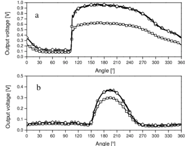
The results were plotted as shown in Fig. 3 depicting typical liquid distribution plots for a rotation of 360o of angle.
B. Identifications of the liquid distributions
Liquid distribution plot was analyzed based on the start and end of bulk liquid. Both start and end of bulk liquid were identified by slope analysis as shown in (1). A Graphical User Interface was created in MATHLAB (R2008b, Mathworks, USA) for an automatic detection of start and end of bulk liquid. The detection of the start of bulk liquid was based on the sharp increase of the slope. The same principle was used to the end of the bulk liquid by detecting the increase of slope but from the opposite direction. The slope was calculated between two consecutive points in each data measurement using the following equation:
1 2
1 2
θ
θ
−
−
=
V
V
m
(1)where m is slope, V2 is second output voltage, V1 is first output voltage,
θ
2is second angle respective to V2 andθ
1is first angle respective to V1. Fig. 3 is an example of a typical of liquid distribution showing the start and end of the bulk liquid at respective heights.The angle positions determined were then plotted in three-dimensional (3D) plots in MATHLAB showing the A
B
D C
I G
J
E F
A B
H
K D
C
45
o
D
C
Emission light to PMT
momentum transfer area of the liquid distribution in shake flask. These are shown in section V with varying filling volumes and viscous conditions ranging from 15 to 40 mL and 0 to 70 g/L of PVP concentration respectively.
0 30 60 90 120 150 180 210 240 270 300 330 360 0.0
0.2 0.4 0.6 0.8 1.0 1.2
O
u
tp
u
t
v
o
lta
g
e
[
V
]
Angle [o
]
0 30 60 90 120 150 180 210 240 270 300 330 360 0.0
0.2 0.4 0.6 0.8 1.0 1.2
O
u
tp
u
t
v
o
lt
a
g
e
[
V
]
Angle [o
]
Fig. 3: Typical liquid distribution plots at different heights for 5 uM fluorescent, pH 8, 100 mM phosphate buffer, 200 rpm of shaking frequency, 25 mm of shaking diameter and 25 ml of filling volume. Symbols in a: ( ) 0.2 cm; ( ) 0.7 cm; ( ) 1.2 cm; ( ) 1.7 cm. Symbols in b: ( ) 2.2 cm; ( ) 2.7 cm; ( ) 3.2 cm; ( ) 3.7 cm; ( ) 4.2 cm. Symbols in (a) and (b): ( ) start of bulk liquid and (/) end of the bulk liquid.
IV.OPTIMIZATIONS OF LIQUID DISTRIBUTION DATA
COLLECTION
The optimizations of the non-invasive technique were investigated on three aspects.
A. Influence of intensity of light emitting diode (LED)
Changing the input voltage of LED changes the level of intensity of LED. The purpose of this was to observe the effect of different input voltage level to the detection of liquid distribution. Experimental conditions of 300 rpm of shaking frequency, 25 mm of shaking diameter and 25 mL of filling volume were implemented.
B. Influence of level of sensitivity of photomultiplier tube
(PMT)
With the increase of the sensitivity level of PMT, the more sensitive the detection of the light emitted from the fluorescent solution. The level of the sensitivity was chosen as such that it was not overloaded being more than maximal output voltage of 10V. The parameters used were at 300 rpm of shaking frequency, 25 mm of shaking diameter and 25 mL of filling volume.
C. Repeatability and reproducibility test
Repeatability and reproducibility of the results were evaluated by the percentage of deviation (PD). The calculations followed in sequence of absolute deviation (ABD) using (2), average deviation (AVD) using (3) and finally percentage deviation (PD) using (4).
The evaluations were conducted at 200 rpm of shaking frequency, 25 mm of shaking diameter and 25 mL of filling
volume based on certain number of rotations of 10, 30, 50, and 100 rotations using the following equations:
] / ) ( [
1
N R R
ABD
N n
n n
=
= −
= , (2)
N ABD AVD
N n
n
/
1
=
=
= , (3)
. 100 ] / ) ( [ /
1
Χ =
=
= N R AVD PD
N n
n
(4) where R is output voltage reading, n is number of reading and N is the total number of different readings.
V. RESULTS AND DISCUSSION
A. Identifications of liquid distributions
Table I shows the degree determined by the slope analysis for the start and end of bulk liquid at different heights only for 200 rpm of shaking frequency, 25 mm of shaking diameter and 25 mL of filling volume as shown in Fig. 3. The degrees were then plotted in angular plots respective to the heights and diameter of the flask.
Table I: List of the degree positions in one rotation for the start and end of bulk liquid.
Heights from bottom [cm]
Start of bulk [degree]
End of bulk [degree]
0.2 93.80 72.50
0.7 85.00 51.40
1.2 83.05 14.35
1.7 90.35 337.50
2.2 103.65 309.10
2.7 121.20 290.10
3.2 149.75 248.65
3.7 171.90 224.85
4.2 0.00 0.00
Having all the degrees plotted at each respective angular plot at each height, the shape of the liquid can be clearly seen for the start and end of bulk liquid as shown in Fig. 4. This represents the shape of liquid sickle and the liquid distribution at the wall of the shake flask.
Fig. 4 specifically shows the increase of the momentum transfer area of the liquid as the filling volume increases. Büchs et al. 2007 showed some shapes of the liquid distribution in shake flask taken by photographs. With these results from this method, the shape of the start of bulk liquid is similar to the shape shown and it justifies the effectiveness a
of the method to determine the liquid distribution in shake flask. This is very useful for further study of the mass transfer of gas-liquid in shake flask during fermentations by investigating the liquid distribution with different viscosity solutions. This is further shown in Fig. 5 showing the liquid distribution for different viscosity conditions in shake flask.
-4 -3 -2 -1 0 1 2 3 4 -4
-2 0
2 4 0
1 2 3 4
X [cm] Y [cm]
Z
[
c
m
]
15 mL 20 mL 25 mL 30 mL 35 mL 40 mL
Fig. 4: Three-dimensional representations of liquid distribution for 5 uM fluorescent solution, pH 8, 100 mM phosphate buffer, 200 rpm of shaking frequency, 25 mm of shaking diameter and at different filling volume ranging from 15 to 40 mL. Symbols: (+) 15 mL; ( ) 20 mL; ( ) 25 mL; ( ) 30 mL; (×) 35 mL; ( ) 40 mL.
-4 -2
0 2
4 -4 -3 -2 -1 0 1 2 3 4
0 0.5 1 1.5 2 2.5 3 3.5
Y [cm] X [cm]
Z
[
cm
]
0 g/L PVP 10 g/L PVP 20 g/L PVP 40 g/L PVP 60 g/L PVP 70 g/L PVP
Fig. 5: Three-dimensional representations of liquid distribution for 5 uM fluorescent solution, pH 8, 100 mM phosphate buffer, 200 rpm of shaking frequency, 25 mm of shaking diameter, 25 mL of filling volume and at different PVP concentrations. Symbols: (+) 0 g/L; ( ) 10 g/L; ( ) 20 g/L; ( ) 40 g/L; (×) 60 g/L; ( ) 70 g/L.
The liquid distributions of different viscous solutions of 0, 10, 20, 40, 60, and 70 g/L of fluorescent-PVP as shown in Fig. 5 depict that as the viscosities increase, the positions of the liquid shift to the right from the reference point at zero coordinate at y-axis (shown as Ref.). The shapes of the liquid sickles for 0, 10, 20, and 40 g/L of fluorescent-PVP remain in-tact, however, the shapes for the liquid sickles for 60 and 70 g/L change most probably due to the change of the rheology of the viscous solutions. It also showed very wide shift of these high viscous solutions of 60 and 70 g/L of fluorescent-PVP solution to the right (counter clockwise direction) from the reference point in reference to 0, 10, 20, and 40 g/L of fluorescent-PVP solution. This may be due to less movement of the liquid in parallel to the orbital shaking
of the shake flask as described as ‘out-of-phase’ condition [5].
B. Intensity of light emitting diodes (LEDs)
Measurements at 1.2 and 3.7 cm for different heights from the base of the flask at varying input voltage of LEDs are shown in Fig. 6. At both positions, liquids circulating in the flask are detected through optical fibers by the PMT. With varying input voltages, the liquid positions especially the start of the bulk liquid are at the same point at both heights. The shapes of the plots are also almost the same having percentage deviations of less than 5% for plots with voltage 4, 4.5, and 5.0 but not for voltage of 3.5 for both heights of 1.2 and 3.7 cm from the base of the flask. For the plot at an input voltage of 3.5, the maximum output voltage is lower than other voltages.
0 30 60 90 120 150 180 210 240 270 300 330 360 0.0
0.1 0.2 0.3 0.4 0.5 0.6 0.7 0.8 0.9 1.0
O
u
tp
u
t
v
o
lt
a
g
e
[
V
]
0 30 60 90 120 150 180 210 240 270 300 330 360 0.0
0.1 0.2 0.3 0.4
0.5 Angle [
o ]
O
u
tp
u
t
v
o
lt
a
g
e
[
V
]
Angle [o]
Fig. 6: Influence of input voltage of LED to the liquid distribution positions for 5 uM fluorescent solution, pH 8, 100 mM phosphate buffer, 300 rpm of shaking frequency, 25 mm of shaking diameter and 25 mL of filling volume at different heights of 1.2 cm (shown in a) and 3.7 cm (shown in b) from the base of the flask. Symbols: ( ) voltage 3.5; ( ) voltage 4.0; ( ) voltage 4.5; ( ) voltage 5.0.
0 30 60 90 120 150 180 210 240 270 300 330 360 0
2 4 6 8
O
u
tp
u
t
v
o
lt
a
g
e
[
V
]
Angle [o
]
0 30 60 90 120 150 180 210 240 270 300 330 360 0
2 4 6 8 10 12
O
u
tp
u
t
vo
lt
a
g
e
[
V
]
Angle [o
]
Fig. 7: Influence of PMT sensitivity level to the liquid distribution positions for 5 uM fluorescent solution, pH 8, 100 mM phosphate buffer, 300 rpm of shaking frequency, 25 mm of shaking diameter and 25 mL of filling volume at different heights of 1.2 cm (shown in a) and 3.7 cm (shown in b) from the base of the flask. Symbols: ( ) sensitivity 1.0; ( ) sensitivity 2.0; ( ) sensitivity 3.0; ( ) sensitivity 4.0; ( ) sensitivity 4.5; ( ) sensitivity 5.0; ( ) sensitivity 6.0.
a Ref.
a
b
Theoretically, the higher the input voltage set up for LED, the higher the intensity of the light. This excites more fluorescent molecules from fluorescent solution resulting in high intensity of emission light being emitted. Therefore, the output voltage becomes higher. Significantly, despite the change of the voltage parameter, the liquid distribution remains the same especially at the start point of the bulk liquid.
C. Level of sensitivity of photomultiplier tube (PMT)
By increasing the level of the sensitivity of PMT, the more sensitive the measurement of the emission light from the fluorescent solution by PMT. Therefore, for both heights of 1.2 and 3.7 cm from the base of the flask, the higher the PMT sensitivity level, the higher the output voltage of the measurements.
From Fig. 7, the liquid distribution plot shapes are the same and the positions of the start of the bulk liquid also remain the same for both heights despite the increase of the PMT sensitivity level. These show that the liquid position measurement is independent of the sensitivity level of PMT except the output voltages of the measurement. For sensitivity level of 6 for height of 1.2 cm from the base of the flask, the output voltage exceeds the maximum allowable output voltage which is 10V read by PMT as shown by the sudden constant line of the plot. Therefore, all measurements of the liquid distributions were run lower than PMT sensitivity of 6.
Liquid distribution also depicts thickness and it varies at different heights of measurement. Thickness of liquid at varying shapes and positions in shake flask is not explained here in this paper. However, the thickness of the liquid influences the intensities of both the fluorescent molecules exposed to the excitation lights and emission lights. In this case, PMT sensitivity of 4.5 was chosen most appropriate applying for all heights of measurement.
0 30 60 90 120 150 180 210 240 270 300 330 360 0.0
0.1 0.2 0.3 0.4 0.5 0.6 0.7
P
e
rc
e
n
ta
g
e
d
e
v
ia
ti
o
n
[
%
]
O
u
tp
u
t
vo
lt
a
g
e
[
V
]
Angle [o
]
-2 -1 0 1 2 3 4 5 6
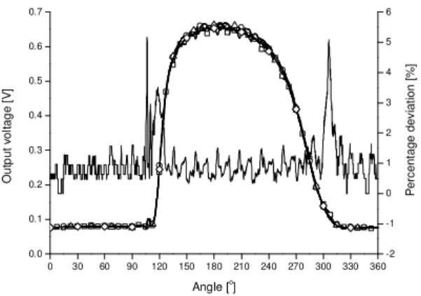
Fig. 8: The percentage of deviations of different number of rotations saved for the measurement for liquid distribution measurement for 5 uM fluorescent solutions, pH 8, 100 mM phosphate buffer, 200 rpm of shaking frequency, 25 mm of shaking diameter and 25 mL of filling volume. Symbols: ( ) 10 rotations; ( ) 30 rotations; ( ) 50 rotations; ( ) 100 rotations.
D. Repeatability and reproducibility
The repeatability and reproducibility of the results are shown by the influence of the number of rotations of the liquid in shake flask in terms of the percentage of deviations. Percentage of deviations of less than 5% is considered acceptable and valid for these evaluations.
Fig. 8 shows that the percentage of deviation approximately less than 5 % for different rotations taken as the mean data measurement. However, there is a very slight abrupt increase of the percentage deviation especially at the start of the bulk liquid most likely due to the sudden detection of the bulk liquid coming to the point where the optical fibers are positioned. All in all, the measurement technique is very reliable for liquid distribution determination.
VI.CONLUSION
The work on the liquid distributions determinations has been done for many conditions and different parameters like shaking frequency, filling volume and viscosity which are not all shown in this paper. This technique has successfully determined the liquid distribution by the detection of the start and end of the bulk liquid. This is very beneficial for the understanding of gas-liquid mass transfer of microorganisms in shake flask during fermentations.
ACKNOWLEDGMENT
The authors acknowledge the Electrical workshop especially Mr. Kosfeld for setting the electrical setup for this measurement, Mechanical workshop for building the setup, Mr. Schemann for programming the LabVIEW program, and Mr. Ranom for programming the Graphical User Interface (GUI) in MATHLAB for automatic liquid distribution determinations. Acknowledgments are also given to the sponsors of the scholarships of Higher Ministry of Education, Malaysia and Deutsche Akademischer Austauch Dienst (DAAD), Germany for the first author and second author respectively.
REFERENCES
[1] U. Maier and J. Büchs. (2001). Characterisation of gas-liquid mass transfer in shaking bioreactors. Biochemical Engineering Journal. 7. pp. 99-106.
[2] U. Maier, M. Losen and J. Büchs. (2004). Advances and understanding and modeling of gas-liquid mass transfer in shake flask. Biochemical Engineering Journal. 17. pp. 155-167.
[3] H.Zhang, W.Williams-Dalson, E. Kesharvarz-Moore and P.A. Shamlou. (2005). Computational-fluid-dynamic (CFD) analysis of mixing and gas-liquid mass transfer in shake flask. Biotechnol. Appl. Biochem. 41.
pp. 1-8.
[4] J. Büchs, U. Maier, S. Lotter and C.P. Peter. (2007). Calculating liquid distribution in shake flask on rotary shakers in waterlike viscosities.
Biochemical Engineering Journal. 34. pp. 200-208.
[5] C.P. Peter, S. Lotter, U. Maier and J. Büchs. (2004). Impact of out-of-phase on screening results in shaking flask experiments.