Hydrol. Earth Syst. Sci., 17, 1561–1573, 2013 www.hydrol-earth-syst-sci.net/17/1561/2013/ doi:10.5194/hess-17-1561-2013
© Author(s) 2013. CC Attribution 3.0 License.
Geoscientiic
Geoscientiic
Hydrology and
Earth System
Sciences
Open Access
Quantifying the uncertainty in estimates of surface–atmosphere
fluxes through joint evaluation of the SEBS and SCOPE models
J. Timmermans1, Z. Su1, C. van der Tol1, A. Verhoef2, and W. Verhoef1
1University of Twente, Faculty for Geoinformation Sciences and Earth Observation (ITC), the Netherlands 2Soil Research Centre, Department of Geography and Environmental Science, The University of Reading, UK Correspondence to:J. Timmermans (j [email protected])
Received: 2 March 2011 – Published in Hydrol. Earth Syst. Sci. Discuss.: 16 March 2011 Revised: 11 February 2013 – Accepted: 3 April 2013 – Published: 22 April 2013
Abstract.Accurate estimation of global evapotranspiration is considered to be of great importance due to its key role in the terrestrial and atmospheric water budget. Global es-timation of evapotranspiration on the basis of observational data can only be achieved by using remote sensing. Several algorithms have been developed that are capable of estimat-ing the daily evapotranspiration from remote sensestimat-ing data. Evaluation of remote sensing algorithms in general is prob-lematic because of differences in spatial and temporal reso-lutions between remote sensing observations and field mea-surements. This problem can be solved in part by using soil-vegetation-atmosphere transfer (SVAT) models, because on the one hand these models provide evapotranspiration esti-mations also under cloudy conditions and on the other hand can scale between different temporal resolutions.
In this paper, the Soil Canopy Observation, Photochem-istry and Energy fluxes (SCOPE) model is used for the eval-uation of the Surface Energy Balance System (SEBS) model. The calibrated SCOPE model was employed to simulate re-mote sensing observations and to act as a validation tool. The advantages of the SCOPE model in this validation are (a) the temporal continuity of the data, and (b) the possibil-ity of comparing different components of the energy balance. The SCOPE model was run using data from a whole growth season of a maize crop.
It is shown that the original SEBS algorithm produces large uncertainties in the turbulent flux estimations caused by parameterizations of the ground heat flux and sensible heat flux. In the original SEBS formulation the fractional vegetation cover is used to calculate the ground heat flux. As this variable saturates very fast for increasing leaf area index (LAI), the ground heat flux is underestimated. It is
shown that a parameterization based on LAI reduces the es-timation error over the season from RMSE=25 W m−2 to
RMSE=18 W m−2. In the original SEBS formulation the
roughness height for heat is only valid for short vegeta-tion. An improved parameterization was implemented in the SEBS algorithm for tall vegetation. This improved the cor-relation between the latent heat flux predicted by the SEBS and the SCOPE algorithm from −0.05 to 0.69, and led to a decrease in difference from 123 to 94 W m−2 for the
la-tent heat flux, with SEBS lala-tent heat being consisla-tently lower than the SCOPE reference. Lastly the diurnal stability of the evaporative fraction was investigated.
1 Introduction
Accurate estimation of evapotranspiration, ET, is considered of great importance due to its key role in hydrology and meteorology. It is involved in many feedback mechanisms, for example between the water and the energy balance, and between the land surface and the atmosphere. Accu-rate estimation of ET is of importance for applications such as irrigation management, weather forecasting and climate model simulations.
global products available are generated using the first two approaches, because of the easy empirical use of remotely sensed land surface temperature and the negligence of mete-orological forcing in the former and the calibration of resis-tances in the latter. With the onset of high performance com-puting and the availability of meteorological fields from large scale models, like GLDAS and ECMWF, the challenges for intensive computation and all related forcing are met paving the way for estimating global evapotranspiration by energy balance models.
Over the last couple of years several initiatives, such as the LandFLUX Initiative (Jim´enez et al., 2011; Mueller et al., 2011), have started to evaluate and develop large scale evapotranspiration products. Low resolution evapotranspi-ration is provided by the Satellite Application Facility on Land Surface Analysis (LandSAF) by feeding geostationary low resolution data into land surface model (Ghilain et al., 2011). Medium resolution calculations of evapotranspiration are performed using orbiting data, from MODIS (Mu et al., 2007, 2011; Vinukollu et al., 2011). However, these products either have a low spatial resolution and high temporal olution or a low temporal resolution and a high spatial res-olution. As such they do not meet the spatial and temporal requirements for a comprehensive water cycle analysis from local to regional scale. In response to the demand for such a product, the Water Cycle Multi-mission Observation Strat-egy (WACMOS), launched by the European Space Agency (ESA), aimed at among others developing a daily evapotran-spiration product on a global scale with a 1km resolution.
It is challenging, for this purpose, to find an algorithm suit-able for the global scale with such high spatial and tempo-ral resolution with sufficient physical characterization. Tri-angle methods (Petropoulos et al., 2009; Jiang et al., 2004) provide good estimations of evapotranspiration for low com-putational requirements, but the chosen algorithm needs to be more physically based to include the most important ex-change processes. Remote sensing based evapotranspiration algorithms, such as TSEB and SEBAL, have difficulties for estimating global evapotranspiration because they require lo-cal lo-calibrations and generate very different estimates (Basti-aanssen et al., 1998; Kustas and Norman, 2000; Timmermans et al., 2007). The Surface Energy Balance System SEBS (Su, 2002) circumvents the calibration problem by using a more physically based parameterization of the turbulent heat fluxes for different states of the land surface and the atmosphere (Su et al., 2001), through implementation of the similarity the-ory (Brutsaert, 1999; Obukhov, 1971; Monin and Obukhov, 1954), while keeping the number of required input variables to a feasible minimum. SEBS thus provides a good compro-mise between the detail levels of the model description on the one hand, and the input requirements. Therefore SEBS is chosen to be the baseline algorithm within the WACMOS project to produce global fluxes.
Like other remote sensing energy balance algo-rithms, SEBS estimates ET from latent heat flux that is
calculated through the evaporative fraction and the available energy. The accuracy of the product thus depends on the accuracy of the other components of the energy balance: net radiation, ground heat flux and sensible heat flux. These components are calculated for the overpass time of the satellite. To scale the estimates up to a daily (24 h) value, an assumption about the diurnal cycle of the fluxes is needed (Rauwerda et al., 2002; Shan et al., 2008).
Validation of ET products is problematic, because spa-tially distributed data for validation are not available. The SEBS algorithm has been validated locally for many low veg-etation types (Shan et al., 2008; Timmermans et al., 2005; Jia et al., 2003; McCabe and Wood, 2006; Su et al., 2005; van der Kwast et al., 2009). Extra uncertainty enters the valida-tion process due to differences in spatial and temporal resolu-tion between the remote sensing observaresolu-tions and the ground measurements (Kite and Droogers, 2000).
Footprints of ground measurements range between 100 m2 and 250 m2for Bowen ratio stations (Pauwels and Samson, 2006; Pauwels et al., 2008) to around 0.1–0.3 km2for scintil-lometer stations (Hartogensis, 2006) up to 0.5 km2for eddy covariance stations (Kljun et al., 2004) depending on the ref-erence height (Schmid, 1997). These scales are much smaller than the desired spatial resolution of the WACMOS project of 1 km2. The required temporal resolution (daily) is diffi-cult to obtain using a single satellite sensor. Combining ob-servations from the Moderate Resolution Imaging Spectrora-diometer (MODIS) and the Advanced Along-Track Scanning Radiometer (AATSR), and the MEdium Resolution Imaging Spectrometer (MERIS) can enhance this temporal resolution, although cloud contamination still is present.
The objective of this paper is to create a methodology for evaluating the suitability of the SEBS model (or any other remote sensing-based evapotranspiration algorithms for that matter) for global application. The application of a calibrated soil-vegetation-atmosphere transfer (SVAT) model (Olioso et al., 1999) would be ideal for such an evaluation. In or-der to create long time series, the input for this SVAT model should be based mostly on meteorological parameters and other field data.
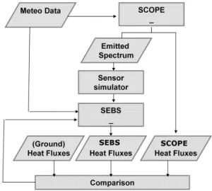
Fig. 1.Methodology for comparing SEBS with SCOPE.
al., 2004), and turbulent heat fluxes were obtained. Finally, the turbulent heat fluxes estimated by the SEBS algorithm were compared to those estimated by the SCOPE model.
In Sect. 2.1 the SEBS and SCOPE model are explained in more detail, as well as the method for coupling the two mod-els together. In Sect. 2.2 the field site and data collection is described, and in Sect. 2.3 the investigations into the leaf area index (LAI) retrieval algorithm and the parameterizations of the different fluxes (ground heat flux, sensible heat flux and daily evapotranspiration) are discussed. The discussion and conclusions follow in the final two sections.
2 Methodology
In this investigation the SCOPE model is coupled to the SEBS model. SCOPE estimates both the turbulent fluxes and hyperspectral radiative transfer. Through a sensor simula-tor and the SEBS preprocessor the input variables for the SEBS algorithm are calculated using the “observations” of band radiances simulated by the SCOPE model. This way the SCOPE model acts as a forcing and validation tool for the SEBS algorithm. This methodology is illustrated in Fig. 1.
The advantage of simulating band radiances enables sim-ulation of remote sensing imagery during cloudy days when actual optical sensors only will measure clouds. This then enables the estimation of evapotranspiration for dates when there is no remote sensing observation and is therefore suit-able for creating long time series. In addition, the capability of simulating remote sensing data from arbitrary sensors can be used to investigate the effectiveness of future satellites, and reanalyze past and current satellite sensor imagery (Tim-mermans et al., 2009; Verhoef, 2008), and to combine several sensors in a synergistic manner. This synergistic use, how-ever, falls outside the scope of the presented investigation.
The investigation into the uncertainties in SEBS flux esti-mates focuses mainly on the effect of high vegetation types on the daily evapotranspiration, because SEBS has so far been validated only for low vegetation types (Shan et al., 2008; Timmermans et al., 2005; Jia et al., 2003; McCabe and Wood, 2006; Su et al., 2005). For high vegetation types some of the parameterizations in SEBS might fail due to the complex nature of the turbulent heat exchange. Focus of this paper will be on the height dependence of the LAI retrieval, the ground heat flux parameterization, the aerodynamic resis-tance estimation, the roughness height for heat transfer, and the diurnal stability of the evaporative fraction.
2.1 SEBS
The Surface Energy Balance System, SEBS, makes use of the energy balance (Eq. 1) to estimate the latent heat flux at the time of overpass. In order to scale from the instantaneous to the daily time scale, it is assumed that the evaporative frac-tion (Eq. 2) remains constant over the day.
Rn=G0+H+λE (1)
3= λE
Rn−G =
3r·λEwet Rn−G
(2)
3r=1−
H−Hwet Hdry−Hwet
(3)
Here, Rn is the net radiation [W m−2]; G0 the soil heat
flux[W m−2];H,H
dry, andHwetare the actual, dry limit and
wet limit sensible heat flux [W m−2], respectively;λE and λEwet are the actual latent heat fluxes [W m−2] at overpass
and the hypothetical wet limit;3and3rare the evaporative
fraction [-] and relative evaporation [-].
SEBS was developed by Su (2002) for the estimation of atmospheric turbulent fluxes using satellite earth observation data. SEBS is often used as a remote sensing algorithm for estimating (daily) evapotranspiration. It consists of a set of algorithms for the determination of the land surface physi-cal parameters and variables, such as albedo, emissivity, land surface temperature, and vegetation coverage, from spectral reflectance and radiance data (Su et al., 1999, 2001; Su, 1996). It includes an extended model for the determination of the roughness height for heat transfer (Su et al., 2001) and a formulation for the estimation of the evaporative fraction on the basis of the energy balance at limiting cases.
In the original formulation, SEBS calculates latent heat flux based on the net radiation, the ground heat flux and the evaporative fraction. The net radiation is calculated using incoming shortwave radiation, albedo, air and land surface temperature and emissivity.
fraction is estimated through the relative evaporation using the sensible heat fluxes (Eqs. 2 and 3). The sensible heat flux is calculated iteratively through use of the Obukhov length and the friction velocity. The equations required to calculate the latent heat flux, ground heat flux and the sensible heat flux are shown in Eqs. (4)–(7).
λE=3 (Rn−G0) (4)
G0=Rn(Ŵc+(1−fc) (Ŵs−Ŵc)) (5)
H=ρaCp
(θo−θa) ra
(6)
ra=
[ln(hcz0h)−Cw]
ku∗ (7)
Herefc is the fractional vegetation cover [-];Ŵc andŴs are
respectively the values for the ratio of the ground heat flux to net radiation for the full canopy limit [-] and the bare soil limit[-];ρais the density of air [kg m−3];Cpis the specific
heat capacity of air [J kg−1K−1];r
ais the aerodynamic
re-sistance [s m−1];u
∗is the friction velocity [s m−1];kis the
von Karman constant [-];θoandθaare the potential
temper-atures of the land surface and air at reference height [K];hc
is the height of the vegetation [m];Cwis the correction term
for atmospheric stability [-], andz0his the roughness height
for heat transfer [m]. The correction term for the atmospheric stability depends on the state of the atmosphere and the mea-surement height. In SEBSCwis calculated using the Monin–
Obukhov Similarity theory (MOS) if the reference height is within the atmospheric surface layer. The Bulk Atmospheric Similarity Theory (BAS) is used if the reference height is above this surface layer and up to the height of the planetary boundary layer. The roughness height for heat transfer is cal-culated based on the roughness height for momentum,z0m,
through the relationship given bykB−1
=ln(z0m/z0h). The kB−1 (Massman, 1999; Su et al., 2001) is calculated based
on the weighted average of limiting values of soil and full canopy (Eq. 8).
kB−1=fc2kBc−1+2fsfckBm−1+fs2kBs−1 (8)
Here, fs is the fractional soil coverage [-]. The bare
soil contribution is calculated as kB−1
s =2.46(Re∗)1/4−
ln(7.4), with Re∗ being the roughness Reynolds num-ber. The full canopy contribution is given by kB−1
c = kCd4Ctβ 1−e−n/2, withCdthe drag coefficient of the
leaves,Ct the heat transfer coefficient of the leaves, β the
ratio between the friction velocity and the wind speed at canopy height, andnthe cumulative leaf drag area. Finally, the soil–canopy interaction contribution is calculated using kB−1
m =kβz0m Ct∗hc, withCt∗the heat transfer coefficient
of the soil.
The errors in the final estimation of evapotranspiration can be attributed to either propagation of input errors, or errors
induced by poor parameterizations of the surface processes in the model. Uncertainties in the input data usually origi-nate from the atmospheric correction of the remote sensing imagery, or from the difference in surface parameter retrieval algorithms. Using the SCOPE model to simulate these vari-ables, such uncertainties are removed in the analysis. 2.2 SCOPE model
The Soil Canopy Observation of Photochemistry and Energy fluxes (SCOPE) model is used to circumvent the above men-tioned problems as it is able to simultaneously simulate top-of-canopy satellite imagery and estimate the evapotranspira-tion. This enables the separation of uncertainties in the input parameters and the errors induced by parameterization errors. The SCOPE model is a soil-vegetation-atmosphere-transfer (SVAT) model that couples radiative soil-vegetation-atmosphere-transfer of op-tical and thermal radiation with leaf biochemistry processes (van der Tol et al., 2009). This coupling is performed, similar to the CUPID model (Norman, 1979), at the leaf level using an energy balance approach model. It calculates the aerody-namic resistances (Verhoef et al., 1999), the within-canopy heat flux vertical distribution, the hyperspectral outgoing ra-diances (Verhoef et al., 2007), the photosynthesis of C3
(Far-quhar et al., 1980) or C4vegetation, and stomatal resistance
(Cowan, 1977).
The radiative transfer of outgoing and internal optical and thermal radiation in SCOPE is based on FluorSAIL with added analytical parts from the unified 4SAIL model (Ver-hoef et al., 2007). This model calculates the directional out-going radiance of the land surface at specific wavelengths, taking into account the spectra of incoming solar and diffuse radiation, canopy structure and the component temperatures of the soil and canopy. The SCOPE model uses a discrete ver-sion of the directional radiative equation to solve the leaf en-ergy balance for different layers (x). In addition, it describes the sun-canopy-observer geometry and on leaf orientation, so that the different biophysical processes for sunlit and shaded components can be considered. The FluorSAIL model orig-inally was intended to compute only canopy reflectance and fluorescence, but the addition of thermal radiation and con-sidering the energy balance on the individual leaf level al-lowed the construction of an SVAT model like SCOPE.
the radiation through the atmosphere, and consequently the simulated radiances are at the top of the canopy.
3 Experimental setup
SCOPE requires measurements of LAI and of incoming op-tical and thermal radiation, air pressure, Ta, wind speed, Ua, and actual vapor pressure, ea. Other variables within
the SCOPE model, like spectral reflectivity and emissiv-ity of the soil/vegetation are set to default values. These data were obtained at The University of Reading Crops Re-search Unit experimental site (Sonning, United Kingdom). A unique feature of this particular dataset is that after the maxi-mum canopy height and LAI (3.7 m2m−2)was achieved the
canopy was thinned out. The LAI values obtained after this thinning were approximately 2.0, 1.0, 0.5 and 0.25 m2m−2.
Leaves were systematically removed from the canopy, with-out modifying the height of the crop. This abrupt change is clearly seen in the different surface parameters (LAI and canopy height) measured, as shown in Fig. 2. The stepwise change in leaf area density provides a perfect dataset for test-ing the variability of the LAI retrieval methods and the effect on the surface energy balance.
The output of SCOPE provides not only the different energy balance components (at different levels within the canopy), but also estimations of the outgoing radiation. As SEBS is a remote sensing algorithm it requires not only the incoming optical and thermal radiation, air temperature, wind speed, and actual vapor pressure, but also the remote sensing imagery like LST and emissivity, fractional vegeta-tion cover and LAI. These remote sensing imagery are calcu-lated on basis of the SCOPE outgoing radiation. SEBS pro-vides then estimations of net radiation, ground heat flux, sen-sible heat flux and latent heat flux.
In addition to the meteorological variables listed above, energy balance components were measured for a complete growth cycle of maize during the summer of 2002 (see van der Tol et al., 2009, for a detailed overview of the site, and sensors used). These energy balance components are com-pared with those estimated by SCOPE and SEBS.
4 Results and discussion
4.1 Leaf area index
The calculation of LAI is not considered part of SEBS core processing, as any LAI products can be used in SEBS. In many researches using SEBS LAI is calculated from NDVI using the parameterization presented in Eq. (9) (Su, 1996), and consequently will be referred to as the original param-eterization. However, this parameterization is only valid for sparse vegetation types; for denser vegetation types it pro-duces values of LAI that are unrealistically high. This can be avoided by coupling LAI to NDVI using a logarithmic
expression (Eq. 10) (Song et al., 2009). These two retrieval algorithms are as follows.
LAI=NDVI r
1+NDVI
1−NDVI (9)
LAI=Aln
1−NDVI B
(10) Here, the values ofAandB depend on the vegetation type, which for maize is given as A=(−2.11)−1 and B
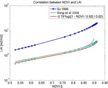
=0.9. NDVI values calculated using the SCOPE outgoing radia-tion, have values higher than 0.9, which would lead to erro-neous values. Consequently, the values forAandB in this logarithmic parameterization should be modified. As proof of the validity of the methodological concept the NDVI val-ues calculated from the SCOPE simulations are compared to the LAI values measured in the field. The results of this comparison are shown in Fig. 3. Here, the original parame-terization by Su, the parameparame-terization by Song et al. (2009) and the parameterization based on Song et al. (2009) but with optimizedAandBvalues, are shown. This optimization re-lied on the reduction of the RMSE between calculated and observed values.
It is clear that the parameterization of Song et al. (2009) with the optimized values, produces more accurate values of LAI than the other two methods. Both relationships between LAI and NDVI given in Su (1996) produce too high results over the whole range of NDVI. For NDVI values close to 0.9, the original by Song et al. (2009) also starts producing too high LAI values. This is because with the original val-ues of Song et al. (2009) the maximum value of NDVI is assumed to be 0.9, while here we find NDVI values as high as 0.92; resulting in non-realistic values. The optimized re-lationship was set for higher maximum NDVI values, and although it produces slightly lower LAI values, the values of LAI do not become infinite for NDVI>0.92. Using these optimized coefficients, the difference between measured and estimated LAI resulted in a RMSE=0.3 m2m−2. It should
be noted that these new values forAandB are not directly applicable to other vegetation types without thorough inves-tigation. It should also be noted that within the WACMOS research the LAI can be obtained from available L2 products. 4.2 Ground heat flux
Fig. 2.SCOPE input parameters and variables measured at the experimental site during 2002. In the top left panel the surface parameters are shown. In the bottom left panel the atmospheric driving variables. In the right panel the incoming optical and thermal radiance data are shown. The red lines depict half hourly in situ measured data, and the blue lines depict the values at AATSR overpass time (Taatsr).
Fig. 3.NDVI – LAI relationships. The LAI values obtained by mea-surements (open circles) and the Su (line with closed circles) and Song parameterizations are shown. The Song parameterization is shown with its original values (the green dotted) forAandB and also for the optimized values (solid red line).
the approach used in Kustas and Daughtry (1989b) as it rep-resents the extinction of the incoming solar radiation within the vegetation more realistically. Values forCr0 and the
ex-tinction coefficienta depend on the vegetation type, but for global application it is usually set to be 0.34 and 0.46, re-spectively (Brutsaert, 2005).
G0 Rn =
Cr0exp(−aLAI) (11)
The values ofCr0andain the current paper are retrieved by
using measured incoming optical and thermal radiation, the outgoing optical and thermal radiation from SCOPE, the land surface temperature obtained through the simulated AATSR sensor and the ground heat flux obtained through
measure-ments. Measurements of outgoing optical and thermal radia-tion are also present but not used in this research, as the pur-pose of this research is to show the synergy between SCOPE and SEBS, in particular when the amount of measured data is minimum. In the SCOPE model the ground heat flux is calculated using a slab model for the ground. Although the modeled soil temperatures are consistent with the observa-tions, the ground heat fluxes are too high compared to the measured values. Therefore, for this investigation the in-situ measurements are used, instead of the simulated values.
In order to achieve a high accuracy, a long time series of both net radiation and ground heat flux is needed, during which LAI does not change. The different classes are filtered, based on the number of values found in the histogram; oc-currences below 50 observations are filtered out. The field in Sonning is therefore well suited for this investigation as the maize was thinned in steps, from very high LAI (3.7 m2m−2)
to very low leaf area index (0.25 m2m−2). Note that only
daytime values between 10:00 and 16:00 LT are used. After filtering the coefficients in Eq. (11) are retrieved. The results are shown in Fig. 4.
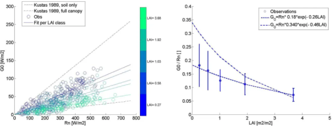
The ratio between the ground heat flux and net radia-tion behaves exactly as predicted; the observaradia-tions fall well within the theoretically predicted values set by the bare soil and full canopy limits. In addition it is observed that the ratio of net radiation and ground heat flux correlates very well with LAI. However, lower values of both the extinction coefficient (a=0.26) and the amplitude (Cro=0.18)are found than the
values advised by (Kustas et al., 1993; Brutsaert, 2005). These low values for the amplitude and the extinction co-efficient originate from the high variation in theRn-G0ratio
Fig. 4.Comparison between the soil heat flux and the net radiation. In the left panel a scatter plot between the net radiation and the ground heat flux is shown for different LAI classes. In this panel also the theoretical limits by Kustas et al. (1993) are shown. The slopes of the fitted data are shown in the right panel. The error bars denote the standard deviation of the retrievedRn-G0ratio. In this panel the parameterization
of Kustas et al. (1993) with original values (dash-dotted) and optimized values (dashed) is also shown.
The high values of the ratio between ground heat flux and net radiation originate for particular sun–leaf geometries, with errors larger than 50 W m−2in G
0for low LAI values.
For these cases the sunbeam directly strikes the soil, without being attenuated by the vegetation. Low values for the ratio between ground heat flux and net radiation originate from low solar zenith angles. For these cases the canopy appears to be dense and closed. These deviations need to be inves-tigated in more detail; therefore, the original values ofCr0
anda given by (Kustas et al., 1993) have been used, instead of the values found by optimization. Using the parameteriza-tion of (Kustas et al., 1993) the difference between observed and measured ground heat flux was 18 W m−2which is a
de-crease when compared original SEBS parameterization with a RMSE=25 W m−2.
4.3 Roughness heights
The sensible heat flux in SEBS is determined by the differ-ence in potential temperature between the land surface and the atmosphere at measurement height and the aerodynamic resistance (Eqs. 6 and 7). This resistance has been shown in the previous section to depend on the roughness height for heat transfer, the friction velocity and the logarithmic pro-file of the wind speed. It was found (Jacobs et al., 1989; Liu et al., 2007b) that the value of aerodynamic resistance for maize ranged from 20 to 50 s m−1. However, when using the
original SEBS parameterizations we found it to vary between 80 and 200 s m−1, resulting in an unrealistically low sensible
heat flux, compared to the measured values.
The error in the aerodynamic resistance appears to be caused by the parameterization of the roughness height for heat transfer. In the original SEBS parameterization this roughness height is estimated based on thekB−1. In SEBS
this variable is usually higher than 8.0; the roughness height for momentum is always higher than the roughness height for heat transfer (i.e.kB−1>0), except for bare soils for which
negative values of kB−1 have been found (see Verhoef et
al., 1997). Small negative values have also been found for tall, dense canopies (Liu et al., 2007a; Jia, 2004). Values for closed canopies are usually around 2, butkB−1increases for
sparse canopies (up to 15 for very sparse canopies), Values of kB−1>8 are therefore deemed too large for the maize crop
with LAI=3.7 m2m−2. However,kB−1values can be
cal-culated from the direct measurements (Liu et al., 2007b) or in our case SCOPE simulations, as shown in Eq. (12).
kB−1
=ρaCp
(Ts−Ta)
H ku∗−ln z
−d0 z0m
+9h z
−d0 L
(12)
HereTsandTaare the temperatures for the land surface and
the atmosphere [K], z is the measurement height [m], do
is the displacement height [m], and9h is the MOS
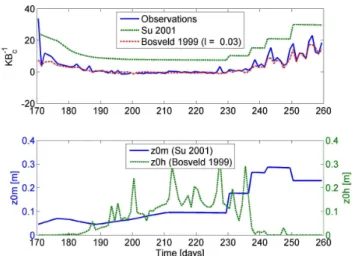
atmo-spheric stability function for heat [-]. The results are shown in Fig. 5. Note the decrease in kB−1 as the canopy height
and density increase throughout the season. The sudden rise in kB−1 around day 230 is caused by the thinning of the
canopy. The minimum value calculated for kB−1
= −0.5. This low value is attributed to the height of the canopy. In high, dense vegetation the incoming radiation only affects the leaf temperature in the upper part of the canopy; in the lower region the radiation is absorbed too much to play a significant role in the temperatures of the leaves (Liu et al., 2007a; Jia, 2004). However, these leaves or twigs still play a role as part of the sink for momentum. This process is well represented in the SCOPE model, as the radiative trans-fer in this model is more accurately represented than in the SEBS model. Hence, instead of the original parameterization forkB−1in SEBS, which produces values that are too high,
Fig. 5.Top panel: seasonal variation in the dailykB−1values for the maize canopy calculated from observations, the parameteriza-tions by Su (2001) and Bosveld et al. (1999). In the bottom panel the roughness length for heat and momentum is shown for Su (2001) and for the newkB−1 parameterization. The new values of the
roughness length for heat, are calculated using thek−1 parameteri-zation of Bosveld (1999), and the roughness length for momentum by Su (2001).
LAI andhc, as in Eq. (13).
kB−1=52
√
u∗l
LAI −0.69 (13)
Here l is the characteristic height for the canopy; in this particular maize canopy the leaf width was measured to be 0.03 m after vegetation stopped growing taller. The temporal variability forkB−1for this method is also shown in Fig. 5,
along with the temporal variability ofkB−1calculated with
the original method employed in SEBS, and with the values based on the SCOPE estimations (Eq. 12).
It is obvious that the new parameterization of kB−1
cor-relates much better with SCOPE estimated values than the original SEBS parameterization. Even the thinning of the LAI is clearly characterized using this method, illustrated by the good correspondence ofkB−1at the end of the
mea-surement period. However the method only applies for closed canopies, and is less accurate for low vegetation. It is there-fore surprising to see that even after the canopy has been thinned to LAI values lower than 1 the parameterization still produces good results (Fig. 6). This could be due to that fact that although leaves are removed from the vegetation, the height of the canopy is left intact. Depending how the leaves were removed the leaf canopy profile might have been al-tered. This can greatly influence the aerodynamic character-istics. As such thinning does not happen in nature it is opted to use this method only for the thresholds set in the origi-nal paper (Bosveld et al., 1999); when the LAI is above the threshold value of 1.5 and only whenhc>1 m.
4.4 Instantaneous heat fluxes
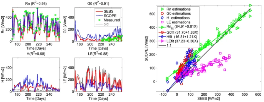
Finally, after implementation of the new parameterizations for high canopy types, the surface heat fluxes can be calcu-lated. The results of these calculations are shown in Fig. 6. In this figure the instantaneous (10:30 LT) net radiation, ground heat flux, sensible heat flux and the latent heat fluxes are shown. All SEBS estimated fluxes, except the latent heat, have a high correlation with the SCOPE estimated values.
– The net radiation of SEBS and SCOPE have a high cor-relation and is fitted with a regression line with slope of 0.81 and a RMSE=54 W m−2. The (optical)
re-flected and thermal radiation as measured for the maize canopy, are very similar to those simulated by SCOPE (not shown); this implies that the land surface temper-ature (LST), albedo and emissivity are retrieved cor-rectly from the SCOPE simulations. This is observed most clearly for day 186 when the differences between measured and modeled net radiation are the highest. The difference in the net radiation arises because SEBS uses air temperature to calculate the longwave incoming ra-diation (Brutsaert, 2005). However, the variation in the downwelling diffuse radiation for medium cloud cov-erage cannot be taken into account using solely the air temperature. Instead the separation of incoming radia-tion into diffuse and direct radiaradia-tion should be based on measurements.
– The ground heat flux calculated by SEBS is much lower than the SCOPE estimated ground heat flux. This is ex-plained in the previous paragraph, and arises because SCOPE estimates the ground heat flux using the force-restore method, which in this case overestimated the ground heat flux. The differences between the measure-ments and the SEBS derived ground heat flux decreased from RMSE=21 W m−2 to RMSE
=18 W m−2 using
the new parameterization. The new SEBS formulation forG0(Brutsaert, 2005; Kustas et al., 1993) clearly
fol-lows the measurements of the ground heat flux. – The SEBS sensible heat flux has improved a lot using
the new parameterization for the roughness height of heat transfer. The differences (expressed as RMSE) be-tween SEBS and SCOPE decreased when using the new parameterization, from 100 to 56 W m−2; the
correla-tion increased from−0.07 to 0.68. Only for high LAI values is SEBS underestimating the sensible heat. This indicates that additional processes play a role in the sen-sible heat flux for high LAI values, other than those al-ready estimated using the new parameterization. – The latent heat flux calculated by SEBS is considerably
Fig. 6.Comparison of instantaneous surface heat fluxes predicted by SEBS and SCOPE. In the left panel the diurnal measurements and estimations are shown. There were no measurements of sensible heat and latent heat over the thinned maize field. In the right panel a scatterplot between SEBS and SCOPE estimated heat fluxes is shown. The instantaneous surface heat fluxes from SEBS show a high correlation with the SCOPE estimated surface heat fluxes. SEBS underestimates the sensible heat flux for a fully developed maize canopy (between day 200 and 220).
Fig. 7.Diurnal variation of the evaporative fraction during the maize growing season. In the left panel the diurnal evaporative fraction as calculated by the SCOPE model for each day is shown. In the right panel the 10 day average of the diurnal evaporative fraction as calculated with SCOPE is shown. The dotted line represents the overpass time of AATSR.
to 94 W m−2. This difference originates mainly due to
low sensible heat fluxes. This results in an overestima-tion of the evaporative fracoverestima-tion for very high LAI. As SEBS does not calculate the latent heat as the energy balance residual, but using the evaporative fraction this also leads to a higher latent heat flux. In Fig. 6 this can be clearly observed because the slope for the sensible heat flux deviates as much from the 1:1 line as the slope of the latent heat flux (but in opposite directions). This will be investigated further in the next section.
4.5 Evaporative fraction
The evaporative fraction, EF, in SEBS is to be calcu-lated based on Eq. (3), but in SCOPE it is calcucalcu-lated as λE(H+λE). In SEBS, EF therefore depends on the actual sensible heat flux, and the sensible heat flux at the hypothet-ical dry and wet limit. The sensible heat flux at these limits is calculated respectively as the maximum available energy, for the dry scenario, while for the wet scenarioH is
calcu-lated fromRn−G0−λE, withλEderived from the Penman
Monteith equation. The evaporative fraction is calculated by SEBS at the time of overpass and considered constant dur-ing the rest of the day. However, several researchers have re-ported a diurnal dependence of the evaporative fraction (Li et al., 2008; Farah et al., 2004; Lu and Zhuang, 2010).
Combining SCOPE and SEBS allows us to investigate not only the diurnal pattern of EF, but also the uncertainties of EF at overpass time and the daily average of EF. The results of the comparison are shown in Fig. 7. Here, the diurnal pattern of the evaporative fraction is shown for the complete growing season, for all individual days (the left panel), and for a 10 day average.
Fig. 8.Variation in evaporative fraction during the maize growing season. Evaporative fractions at overpass time calculated by SEBS and SCOPE are shown, as well as the daily average values of the evaporative fraction by SCOPE.
240–250 and 250–260. These days correspond to low LAI values of 0.25, 0.5 and 0.25, respectively. For days 230–240, (LAI=1.0) the evaporative fraction starts to vary diurnally. For all other days (i.e. those with LAI>1.0) EF has a pro-nounced diurnal pattern. For LAI>2.0 EF has the same pat-tern: with EF lower in the morning than later in the day. Therefore, the values of the average evaporative fraction are higher than the values of the instantaneous evaporative frac-tion. This is confirmed in Fig. 7.
Figure 8 shows both the instantaneous evaporative frac-tions at overpass time calculated by SEBS and SCOPE and the daily average values of the evaporative fraction calcu-lated by SCOPE. The daily evaporative fraction is in all cases higher than the instantaneous EF by SCOPE, except for the low LAI classes (at the very start and end of the experimental period). The comparison between instantaneous/daily aver-age evaporative fractions by SEBS and SCOPE is hampered due to the large variation in the SEBS evaporative fraction. This variation occurs when net radiation is very low. In these cases the evaporative fraction calculated by SEBS becomes very low. The explanation of this low net radiation was given in the previous paragraph. When only taking into account the moderate and high values the instantaneous evaporative frac-tion by SEBS is much higher than the instantaneous evapo-rative fraction of SCOPE. This is due to an underestimation of the sensible heat for high LAI values, which should be ex-plored in future investigations. Fortunately, when comparing the instantaneous evaporative fraction values with the daily averaged ones they are of the same order. For sensors with different overpass times, however, it could lead to an extra uncertainty, although this diurnal pattern is only apparent for low radiation values.
5 Conclusions
In this paper a method was successfully presented for the validation/investigation of the SEBS model, or any other re-mote sensing model that calculates energy balance fluxes and surface temperatures. This method uses the SCOPE model to estimate simultaneously the turbulent heat fluxes from a canopy as well as band observations from a satellite sensor. These radiances were then fed through the SEBS prepro-cessor in order to obtain surface variables like LST, albedo and emissivity. The data used for this comparison comprised micrometeorological forcing data and verification data for a complete growing season of maize.
Parameterizations investigated were the LAI retrieval al-gorithm, the ground heat flux parameterization and the esti-mation of the roughness height for heat transfer (this plays a role in the aerodynamic resistance). For each of these param-eterizations there were problems at high values of LAI. It was found that the original LAI parameterization in SEBS over-estimated LAI. The method proposed by Song et al. (2009) was used instead, as this fitted very well with the observa-tions for most LAI classes. This algorithm was slightly al-tered to incorporate the high NDVI values estimated for the maize canopy under study. The new algorithm showed lower errors (RMSE=0.3 m2m−2) than the parameterization
cur-rently implemented in the SEBS algorithm.
The original parameterization of the ground heat flux used the fractional vegetation cover in a weighted average ap-proach. As fractional vegetation cover saturates more quickly with vegetation growth than the maximum canopy height and LAI, it was decided to change this parameterization. Be-cause currently SCOPE overestimates the ground heat flux, the ground heat flux from measurements was used to cali-brate an alternative, more physical, parameterization (Kustas and Daughtry, 1989a); it characterizes the extinction of radi-ation through a dense canopy. Values for the different coef-ficients were obtained through investigating the ratio of soil heat flux and net radiation for different LAI classes. Varia-tions in the coefficients originated because the measured val-ues for low LAI valval-ues showed high variation. Therefore, in-stead of using the optimized coefficients, it was decided to use the original Kustas parameter values.
The last parameterization modified was that describing the relative magnitude of the roughness height for momentum and heat transfer, as expressed by the parameter kB−1
=
ln(z0m/z0h). In high dense canopies most of the radiation
is absorbed by the leaves at the top of the canopy. Therefore, the position of the virtual source of the sensible heat, as ex-pressed byz0h, is relatively higher in the canopy than for low
of the correlation between SEBS and SCOPE modeled sen-sible heat flux from−0.07 to 0.68.
After implementing all the new parameterizations, the var-ious energy balance fluxes and the evaporative fraction were calculated. Even though the roughness height for heat was improved greatly using a new parameterization, SEBS still underestimated the sensible heat flux for high LAI values. This means that some processes are still not characterized well enough and further investigation is required. Using the instantaneous, wet and dry limit sensible heat fluxes, the evaporative fraction, EF, was calculated in SEBS. This EF was compared to the instantaneous and daily averaged EF simulated by SCOPE. SCOPE calculated a diurnal pattern in the evaporative fraction causing the daily average to be higher than the SCOPE-obtained instantaneous EF at over-pass time. EF from SEBS however was of the same order as the SCOPE daily averaged evaporative fraction. This orig-inates from the low values of the SEBS estimated instan-taneous sensible heat. Although the new parameterization forkB−1over tall vegetation can still be improved further,
estimations by SEBS can already be used for daily evap-otranspiration estimations because the obtained valued for the evaporative fraction appears to represent correctly the daily average.
In conclusion, the methodology presented in this paper en-abled a thorough investigation in the different parameteriza-tions of SEBS. The advantage of the method presented in this paper, i.e. combining SEBS with SCOPE, is mainly that for days where there are no acquisitions we can still con-duct the investigation. Although no actual remote sensing imagery was used, the methodology, through the use of the sensor simulator, proved the viability of using the AATSR sensor for calculating the different land surface fluxes. While the SCOPE has been tested over maize and forest to pro-vide good estimations of the fluxes it has not been validated over other vegetation types. This will be necessary to use this methodology in other areas. Finally, the SCOPE model at the moment overestimates the ground heat flux; this should be addressed in the next version of the SCOPE model. A version of SCOPE that incorporates a detailed multi-layer below-ground parameterization of heat, water and gas fluxes will be developed in the context of the UK (NERC) funded FUSE project (NE/I007288/1).
Acknowledgements. We would like to thank the ESA for funding the reported research through the WACMOS project. Kitsiri Weligepolage is thanked for his help with the parameterization of the roughness height for heat. Furthermore, various people were involved during the fieldwork at Sonning farm. Special thanks are due to Caroline Houldcroft and Bruce Main.
Edited by: H. Cloke
References
Bastiaanssen, W. G. M., Menenti, M., Feddes, R. A., and Holtslag, A. A. M.: A remote sensing surface energy balance algorithm for land (SEBAL). 1. Formulation, J. Hydrol., 212–213, 198–212, 1998.
Bosveld, F., Holtslag, A. A. M., and Van Den Hurk, B. J. J. M.: In-terpretation of Crown Radiation Temperatures of a Dense Dou-glas fir Forest with Similarity Theory, Bound.-Layer Meteor., 92, 429–451, doi:10.1023/a:1002087526720, 1999.
Brutsaert, W.: Aspects of Bulk Atmospheric Boundary Layer Sim-ilarity Under Free-Convective Conditions, Rev. Geophys., 37, 439–451, doi:10.1029/1999rg900013, 1999.
Brutsaert, W.: Hydrology, Cambridge University Press, New york, 605 pp., 2005.
Carlson, T.: An Overview of the “Triangle Method” for Estimat-ing Surface Evapotranspiration and Soil Moisture from Satellite Imagery, Sensors, 7, 1612–1629, 2007.
Cowan, I.: Stomatal behaviour and environment, Adv. Bot. Res. 4, 114–228, 1997
Farah, H. O., Bastiaanssen, W. G. M., and Feddes, R. A.: Eval-uation of the temporal variability of the evaporative fraction in a tropical watershed, Inte. J. Appl. Earth Obs., 5, 129–140, doi:10.1016/j.jag.2004.01.003, 2004.
Farquhar, G. D., Caemmerer, S, and Berry, J. A.: A biochemi-cal model of photosynthetic CO2assimilation in leaves of C3
species, Planta, 149, 78–90, 1980.
Ghilain, N., Arboleda, A., and Gellens-Meulenberghs, F.: Evapo-transpiration modelling at large scale using near-real time MSG SEVIRI derived data, Hydrol. Earth Syst. Sci., 15, 771–786, doi:10.5194/hess-15-771-2011, 2011.
Glenn, E. P., Huete, A. R., Nagler, P. L., Hirschboeck, K. K., and Brown, P.: Integrating remote sensing and ground methods to es-timate evapotranspiration, CRC Cr. Rev. Plant Sci., 26, 139–168, doi:10.1080/07352680701402503, 2007.
Hartogensis, O.: Exploring Scintillometry in the Stable Atmo-spheric Surface Layer, PhD, Meteorologie en Luchtkwaliteit, Wageningen Universiteit, Wageningen, 240 pp., 2006.
Jacobs, A. F. G., Halbersma, J., and Przybula, C.: Behaviour of Crop resistance of maize during a growing season, Estimation of Areal Evapotranspiration, Vancouver, Canada, 1989.
Jia, L.: Modeling heat exchanges at the land-atmosphere interface using multi-angular thermal infrared measurements, Ph.D, Wa-geningen University, WaWa-geningen, 199 pp., 2004.
Jia, L., Su, Z. B., van den Hurk, B., Menenti, M., Moene, A., De Bruin, H. A. R., Yrisarry, J. J. B., Ibanez, M., and Cuesta, A.: Es-timation of sensible heat flux using the Surface Energy Balance System (SEBS) and ATSR measurements, Phys. Chem. Earth, 28, 75–88, doi:10.1016/s1474-7065(03)00009-3, 2003. Jiang, L., Islam, S., and Carlson, T. N.: Uncertainties in latent heat
flux measurement and estimation: implications for using a sim-plified approach with remote sensing data, Can. J. Remote Sens., 30, 769–787, doi:10.5589/m04-038, 2004.
Kalma, J. D., McVicar, T. R., and McCabe, M. F.: Estimating Land Surface Evaporation: A Review of Methods Using Remotely Sensed Surface Temperature Data, Surv. Geophys., 29, 421–469, doi:10.1007/s10712-008-9037-z, 2008.
Kite, G. W. and Droogers, P.: Comparing evapotranspiration esti-mates from satellites, hydrological models and field data, J. Hy-drol., 229, 3–18, 2000.
Kljun, N., Calanca, P., Rotach, M., and Schmid, H.: A Simple Pa-rameterisation for Flux Footprint Predictions, Bound.-Lay. Mete-orol., 112, 503–523, doi:10.1023/b:boun.0000030653.71031.96, 2004.
Kustas, W. P. and Daughtry, C. S. T.: Estimation of the soil heat flux/ net radiation ratio from spectral data, Agr. Forest Meteorol., 49, 205–223, 1989a.
Kustas, W. P. and Daughtry, C. S. T.: Estimation of the soil heat flux/net radiation from spectral data, Agric. For. Meteorol., 49, 205–223, 1989b.
Kustas, W. P. and Norman, J. M.: A Two-Source Energy Balance Approach Using Directional Radiometric Temperature Observa-tions for Sparse Canopy Covered Surfaces, Agron. J., 92, 847– 854, 2000.
Kustas, W. P., Daughtry, C. S. T., and Oevelen, P.: Analytical treat-ment of the relationships between soil heat flux/net radiation ra-tio and vegetara-tion indices, Remote sensing of environment, 46, 319–330, 1993.
Li, S., Kang, S., Li, F., Zhang, L., and Zhang, B.: Vineyard evapo-rative fraction based on eddy covariance in an arid desert region of Northwest China, Agr. Water Manage., 95, 937–948, 2008. Liu, Q. H., Huang, H. G., Qin, W. H., Fu, K. H., and
Li, X. W.: An extended 3-D radiosity-graphics combined model for studying thermal-emission directionality of crop canopy, IEEE Trans. Geosci. Remote Sens., 45, 2900–2918, doi:10.1109/tgrs.2007.902272, 2007a.
Liu, Shaomin, Lu, L., Mao, D., and Jia, L.: Evaluating param-eterizations of aerodynamic resistance to heat transfer using field measurements, Hydrol. Earth Syst. Sci., 11, 769–783, doi:10.5194/hess-11-769-2007, 2007b.
Lu, X. and Zhuang, Q. L.: evaluating evapotranspiration and wa-ter use efficiency of wa-terrestrial ecosystems in the conwa-terminous united states using modis and ameriflux, Remote Sens. Environ., 114, 1924–1939, 2010.
Massman, W. J.: A model study of kBH-1 for vegetated surfaces using [“]localized near-field” Lagrangian theory, J. Hydrol., 223, 27–43, 1999.
McCabe, M. F. and Wood, E. F.: Scale influences on the remote estimation of evapotranspiration using multiple satellite sensors, Remote Sens. Environ., 105, 271–285, doi:10.1016/j.rse.2006.07.006, 2006.
McNaughton, K. G. and van den Hurk, B. J. J. M.: A “Lagrangian” revision of the resistors in the two-layer model for calculating the energy budget of a plant canopy, Bound.-Layer Meteor., 74, 261–288, 1995.
Monin, A. S. and Obukhov, A. M.: Osnovnye zakonomernosti turbulentnogo peremesivanija v prizemnom sloe atmosfery, Trudy geofiz. inst. AN SSSR, 24, 163–187, citeulike-article-id:3716139, 1954.
Monteith, J. L.: Principles of environmental physics, edited by: Press, E. A., 1973.
Mu, Q., Heinsch, F. A., Zhao, M., and Running, S. W.: Development of a global evapotranspiration algorithm based on MODIS and global meteorology data, Remote Sens. Environ., 111, 519–536, doi:10.1016/j.rse.2007.04.015, 2007.
Mu, Q., Zhao, M., and Running, S. W.: Improvements to a MODIS global terrestrial evapotranspiration algorithm, Remote Sens. En-viron., 115, 1781–1800, doi:10.1016/j.rse.2011.02.019, 2011. Mueller, B., Seneviratne, S. I., Jimenez, C., Corti, T., Hirschi, M.,
Balsamo, G., Ciais, P., Dirmeyer, P., Fisher, J. B., Guo, Z., Jung, M., Maignan, F., McCabe, M. F., Reichle, R. H., Reichstein, M., Rodell, M., Sheffield, J., Teuling, A. J., Wang, K., Wood, E. F., and Zhang, Y.: Evaluation of global observations-based evapo-transpiration datasets and IPCC AR4 simulations, Geophys. Res. Lett., doi:10.1029/2010GL046230, 38, L06402, 2011.
Norman, J. M.: Modeling the complete crop canopy, in: Modifica-tion of the aerial environment of plants, edited by: Barfield, B. J. and Gerber, J. F., ASAE Monogr. Am. Soc. Agric. Eng., St. Joseph, MI., 249–277, 1979.
Obukhov, A. M.: Turbulence in an atmosphere with a non-uniform temperature, Bound.-Lay. Meteorol., 2, 7–29, 1971.
Olioso, A., Chauki, H., Wigneron, J., Bergaoui, K., Bertuzzi, P., Chanzy, A., Bessemoulin, P., and Clavet, J. C.: Estimation of energy fluxes from thermal infrared, spectral reflectances, mi-crowave data and SVAT modeling, Phys. Chem. Earth B, 24, 829–836, 1999.
Pauwels, V. R. N. and Samson, R.: Comparison of different methods to measure and model actual evapotranspiration rates for a wet sloping grassland, Agr. Water Manage., 82, 1–24, doi:10.1016/j.agwat.2005.06.001, 2006.
Pauwels, V. R. N., Timmermans, W., and Loew, A.: Comparison of the estimated water and energy budgets of a large winter wheat field during AgriSAR 2006 by multiple sensors and models, J. Hydrol., 349, 425–440, doi:10.1016/j.jhydrol.2007.11.016, 2008.
Petropoulos, G., Carlson, T. N., Wooster, M. J., and Islam, S.: A review of Ts/VI remote sensing based methods for the retrieval of land surface energy fluxes and soil surface moisture, Progr. Phys. Geogr., 33, 224–250, doi:10.1177/0309133309338997, 2009. Rauwerda, J., Roerink, G. J., and Su, Z.: Estimation of evaporative
fractions by the use of vegetation and soil component tempera-tures determined by means of dual-looking remote sensing, Wa-geningen, Alterra, Green World Research, 149, 2002.
Schmid, H. P.: Experimental design for flux measurements: match-ing scales of observations and fluxes, Agric. For. Meteorol., 87, 179–200, doi:10.1016/S0168-1923(97)00011-7, 1997.
Shan, X., van de Velde, R., Wen, J., He, Y., Verhoef, W., and Su, Z.: Regional Evapotranspiration over the arid inland heihe river basin in northwest China, Dragon 1 Programme Final Results, Beijing, 2008.
Sobrino, J. A., Soria, G., and Prata, A. J.: Surface temperature re-trieval from Along Track Scanning Radiometer 2 data: Algo-rithms and validation, J. Geophys. Res.-Atmos., 109, D11101, doi:10.1029/2003jd004212, 2004.
Song, J., Wang, J., Xiao, Z., and Xiao, Y.: The method on generating LAI production by fusing BJ-1 remote sensing data and modis LAI product, Geoscience and Remote Sensing Symposium,2009 IEEE International,IGARSS 2009, IV-825-IV-828, 2009. Su, H., McCABE, M. F., and Wood, E. F.: Modeling
for Local- and Regional-Scale Prediction, J. Hydrometeorol., 6, 910–922, 2005.
Su, Z.: Remote Sensing Applied to Hydrology: The Sauer River Basin Study, Ph.D, Hydrologie/Wasserwirtschaft, Faculty of Civil Engineering, Ruhr Univesity, Bochum, 1996.
Su, Z.: The Surface Energy Balance System (SEBS) for estima-tion of turbulent heat fluxes, Hydrol. Earth Syst. Sci., 6, 85–100, doi:10.5194/hess-6-85-2002, 2002.
Su, Z., Pelgrum, H., and Menenti, M.: Aggregation effects of sur-face heterogeneity in land sursur-face processes, Hydrol. Earth Syst. Sci., 3, 549–563, doi:10.5194/hess-3-549-1999, 1999.
Su, Z., Schmugge, T., Kustas, W. P., and Massman, W. J.: An evalua-tion of two models for estimaevalua-tion of the roughness height for heat transfer between the land surface and the atmosphere, J. Appl. Meteorol., 40, 1933–1951, 2001.
Timmermans, J., Verhoef, W., van der Tol, C., and Su, Z.: Retrieval of canopy component temperatures through Bayesian inversion of directional thermal measurements, Hydrol. Earth Syst. Sci., 13, 1249–1260, doi:10.5194/hess-13-1249-2009, 2009. Timmermans, W. J., van der Kwast, J., Gieske, A. S. M., Su, Z.,
Olioso, A., Jia, L., and Elbers, J. A.: Intercomparison of Energy Flux Models using Aster Imagery at the SPARC 2004 site (Bar-rax, Spain), SPARC final workshop, Enschede, 2005.
Timmermans, W. J., Kustas, W. P., Anderson, M. C., and French, A. N.: An intercomparison of the surface energy balance al-gorithm for land (SEBAL) and the two-source energy balance (TSEB) modeling schemes, Remote Sens. Environ., 108, 369– 384, doi:10.1016/j.rse.2006.11.028, 2007.
van der Kwast, J., Timmermans, W., Gieske, A., Su, Z., Olioso, A., Jia, L., Elbers, J., Karssenberg, D., and de Jong, S.: Eval-uation of the Surface Energy Balance System (SEBS) applied to ASTER imagery with flux-measurements at the SPARC 2004 site (Barrax, Spain), Hydrol. Earth Syst. Sci., 13, 1337–1347, doi:10.5194/hess-13-1337-2009, 2009.
van der Tol, C., Verhoef, W., Timmermans, J., Verhoef, A., and Su, Z.: An integrated model of soil-canopy spectral radiances, pho-tosynthesis, fluorescence, temperature and energy balance, Bio-geosciences, 6, 3109–3129, doi:10.5194/bg-6-3109-2009, 2009. Verhoef, A., McNaughton, K. G., and Jacobs, A. F. G.: A parameter-ization of momentum roughness length and displacement height for a wide range of canopy densities, Hydrol. Earth Syst. Sci., 1, 81–91, doi:10.5194/hess-1-81-1997, 1997.
Verhoef, W.: A Bayesian optimisation approach for model inver-sion of hyperspectral – multidirectional observations: the bal-ance with A Priori information, 10th international symposium on physical measurements and spectral signatures in remote sens-ing, Davos, Switserland, 208–213, 2008.
Verhoef, W. and Bach, H.: Coupled soil-leaf-canopy and atmosphere radiative transfier modeling to simulate hy-perspectral multi-angular surface reflectance and TOA radiance data, Remote Sens. Environ., 109, 166–182, doi:10.1016/j.rse.2006.12.013, 2007.
Verhoef, W., Jia, L., Xiao, Q., and Su, Z.: Unified optical-thermal four-stream radiative transfer theory for homogeneous vegetation canopies, IEEE Trans. Geosci. Remote Sens., 45, 1808–1822, doi:10.1109/tgrs.2007.895844, 2007.